Cleveland State University
EngagedScholarship@CSU
ETD Archive2014
Oppositional Biogeography-Based Optimization
Mehmet Ergezer
Cleveland State University
Follow this and additional works at:https://engagedscholarship.csuohio.edu/etdarchive Part of theElectrical and Computer Engineering Commons
How does access to this work benefit you? Let us know!
This Dissertation is brought to you for free and open access by EngagedScholarship@CSU. It has been accepted for inclusion in ETD Archive by an authorized administrator of EngagedScholarship@CSU. For more information, please [email protected].
Recommended Citation
Ergezer, Mehmet, "Oppositional Biogeography-Based Optimization" (2014).ETD Archive. 90.
O
PPOSITIONAL
B
IOGEOGRAPHY
-B
ASED
O
PTIMIZATION
M
EHMET
E
RGEZER
Bachelor of Engineering in Electrical and Computer Engineering Youngstown State University
May, 2003
Master of Science in Electrical and Computer Engineering Youngstown State University
May, 2006
submitted in partial fulfillment of the requirements for the degree
DOCTOR OF ENGINEERING
at the
CLEVELAND STATE UNIVERSITY
May 2014
c
We hereby approve the dissertation of
Mehmet Ergezer
Candidate for the Doctor of Engineering degree. This dissertation has been approved for the Department of Electrical and Computer Engineering
and CLEVELAND STATE UNIVERSITY College of Graduate Studies by
Dan Simon, Dissertation Committee Chairperson
Department/Date
Murad Hizlan, Dissertation Committee Member
Department/Date
Hanz Richter, Dissertation Committee Member
Department/Date
Iftikhar Sikder, Dissertation Committee Member
Sailai Shao, Dissertation Committee Member
Department/Date
Dan Simon, Doctoral Program Director
Department/Date
Chansu Yu, Department Chair
Department/Date
ACKNOWLEDGMENTS
T
HEREare many people that I would like to thank for their help and sup-port to help me become the person that I am today. Foremost, I must acknowledge my adviser Dr. Simon for always leading by example, through his hard work and ethical and optimal decision making skills. I am forever grateful to him for his mentoring style of encouraging investigative thinking and allowing us the freedom to do research.It gives me great pleasure in acknowledging the support and help of all my committee members, Dr. Hizlan, Dr. Richter, Dr. Sikder and Dr. Shao for all their suggestions and recommendations.
Special thanks to Dawei Du, Rick Rarick, George Thomas, Berney Mon-tavon, Paul Lozovyy and all of the remaining past and present members of the Embedded Controls Lab. Being part of a team that solves real-world problems has been one of the most rewarding experiences of my life. Also, many thanks to our industrial partners, including Jeff Abell from General Motors, Nick Ma-standrea from Innovative Developments and Arun Venkatesan from Cleveland Medical Polymers, for working with us on these projects.
I consider it an honor to work with my fellow engineers at ARCON Cor-poration. I am indebted to them for encouraging me the complete my research. Last, but not least, I owe a debt of gratitude to my family, especially my parents Güngör and Dr. Yalçın Ergezer. I could not achieve this without their unconditional love, encouragement and guidance. I must also thank Slava and her parents for welcoming me and tolerating me through this long adventure and for providing me with the much needed relief from the technical world.
O
PPOSITIONAL
B
IOGEOGRAPHY
-B
ASED
O
PTIMIZATION
MEHMET ERGEZER
ABSTRACT
T
HIS dissertation outlines a novel variation of biogeography-based opti-mization (BBO), which is an evolutionary algorithm (EA) developed for global optimization. The new algorithm employs opposition-based learning (OBL) alongside BBO migration to create oppositional BBO (OB B O). Addition-ally, a new opposition method named quasi-reflection is introduced. Quasi-reflection is based on opposite numbers theory and we mathematically prove that it has the highest expected probability of being closer to the problem solu-tion among all OBL methods that we explore. Performance of quasi-opposisolu-tion is validated by mathematical analysis for a single-dimensional problem and by simulations for higher dimensions. Experiments are performed on benchmark problems taken from the literature as well as real-world optimization problems provided by the European Space Agency. Empirical results demonstrate that with the assistance of quasi-reflection, OB B O significantly outperforms BBO in terms of success rate and the number of fitness function evaluations required to find an optimal solution for a set of standard continuous domain benchmarks.The oppositional algorithm is further revised by the addition of fitness-dependent quasi-reflection which gives a candidate solution that we callxˆKr. In
this algorithm, the amount of reflection is based on the fitness of the individual and can be non-uniform. We find that for small reflection weights, xˆKr has
In addition, we extend the idea of opposition to combinatorial problems. We introduce two different methods of opposition to solve two types of com-binatorial optimization problems. The first technique, open-path opposition, is suited for combinatorial problems where the final node in the graph does not have be connected to the first node such as the graph-coloring problem. The latter technique, circular opposition, can be employed for problems where the endpoints of a graph are linked such as the well-known traveling sales-man problem (TSP). Both discrete opposition methods have been hybridized with biogeography-based optimization (BBO). Simulations on standard graph-coloring and TSP benchmarks illustrate that incorporating opposition into BBO improves performance.
TABLE OF CONTENTS
Page
ABSTRACT vi
LIST OF TABLES xii
LIST OF FIGURES xv
CHAPTER
I. INTRODUCTION 1
1.1 Evolutionary Computation . . . 2
1.1.1 History of Evolutionary Computation . . . 2
1.1.2 Evolutionary Computation Methodology . . . 6
1.1.3 Controversies and No Free Lunch Theorem . . . 7
1.1.4 Evolutionary Computation Applications. . . 8
1.2 Biogeography-based Optimization . . . 8 1.3 Opposition-based Learning . . . 11 1.4 Algorithms . . . 14 1.4.1 Genetic Algorithms . . . 16 1.4.2 Differential evolution . . . 18 1.4.3 Biogeography-based Optimization . . . 19
1.5 Motivation for this Research . . . 20
1.6 Contributions of This Research . . . 21
II. PROBABILISTIC ANALYSIS OF OPPOSITION-BASED LEARNING 23 2.1 Definitions of Oppositional Points . . . 23
2.4 Distance Between a Fitness-Dependent Quasi-Reflected Point and the Solution. . 33
2.5 Summary . . . 36
2.5.1 Probabilities . . . 36
2.5.2 Expected Distance of Fitness-Weighted Quasi-Reflection Compared to an EA Individual . . . 37
III. EMPIRICAL RESULTS OF OPPOSITION-BASED LEARNING 40 3.1 Simulation Settings . . . 41
3.2 Benchmark Functions . . . 43
3.2.1 Low-dimensional Benchmark Problems . . . 44
3.2.2 Variable-dimension Benchmark Problems . . . 44
3.3 Simulation Results . . . 46
3.3.1 Experimental Comparison of Oppositional Algorithms . . . 46
3.3.2 Reflection Range . . . 54
3.4 Real-world problems . . . 58
3.5 Simulation Settings . . . 59
3.6 Simulation Results . . . 60
3.7 Statistical Tests . . . 64
IV. DISCRETE AND COMBINATORIAL OPPOSITION 67 4.1 Open-path Opposition . . . 68
4.2 Cycle Opposition . . . 71
4.3 Combinatorial Biogeography-based Optimization . . . 76
4.4 Experimental Results . . . 77
4.4.1 Vertex Coloring . . . 77
4.4.2 Traveling Salesman Problem . . . 81
4.5 Conclusions on Combinatorics . . . 84
V. CONCLUSIONS AND FUTURE WORK 86 5.1 Opposition Probabilities in Higher Dimensions. . . 87
5.2 Constrained Optimization. . . 89
5.3 Biogeographical Extensions . . . 91
APPENDICES 96 A. PROOFS 97 A.1 Quasi-Opposition vs. Opposite . . . 97
A.2 Quasi-Reflection vs. Opposite . . . 102
A.3 Quasi-Opposition vs. EA Individual . . . 105
A.4 Quasi-Reflection vs. EA Individual . . . 109
A.5 Probabilistic Analysis of Fitness-Weighted Quasi-Reflection . . . 111
A.5.1 Case (A) . . . 112
A.5.2 Case (B) . . . 112
A.5.3 Case (C) . . . 116
A.5.4 Case (D) . . . 117
A.5.5 Conditional Probability . . . 117
A.5.6 Probability . . . 118
A.6 Expected Distance of Fitness-Weighted Quasi-Reflected Point . . . 118
A.6.1 Probability Distribution Functions . . . 118
A.6.2 Distance betweenxˆKrandx . . . 120
A.6.3 Absolute Value of Distance betweenxˆKrandx . . . 124
A.6.4 Expected Distance betweenxˆKrandx . . . 125
A.6.5 Distance betweenxˆandx. . . 126
A.6.6 Absolute Value of Distance betweenxˆandx. . . 129
A.6.7 Expected Distance betweenxˆandx . . . 129
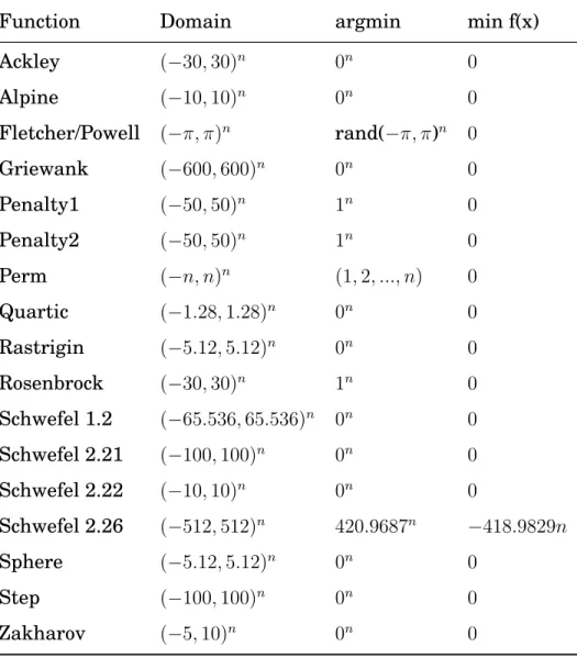
B. BENCHMARK FUNCTIONS 131 B.1 Low-Dimensional Benchmark Problems . . . 131
B.1.3 DeJong F5 . . . 133
B.1.4 Easom . . . 134
B.1.5 Perm . . . 135
B.1.6 Tripod . . . 136
B.2 Variable-Dimensional Benchmark Problems . . . 138
B.2.1 Ackley . . . 138 B.2.2 Alpine . . . 139 B.2.3 Fletcher/Powell . . . 140 B.2.4 Griewangk . . . 141 B.2.5 Penalty 1 . . . 142 B.2.6 Penalty2 . . . 143 B.2.7 Quartic . . . 145 B.2.8 Rastrigin . . . 146 B.2.9 Rosenbrock . . . 147 B.2.10 Schwefel 1.2 . . . 148 B.2.11 Schwefel 2.21 . . . 149 B.2.12 Schwefel 2.22 . . . 150 B.2.13 Schwefel 2.26 . . . 151 B.2.14 Sphere . . . 152 B.2.15 Step . . . 153 B.2.16 Zakharov . . . 154
C. PUBLISHED, PRESENTED, AND SUBMITTED RESULTS FROM THIS
RESEARCH 155
LIST OF TABLES
Table Page
I Degrees of opposition . . . 27
II Examples of reflection weights . . . 31
III Probability that opposite point is closer than an EA individ-ual to the solution of an optimization problem. . . 36
IV Distance to solution as a function of reflection weight . . . 38
V Problem dimension vs. population size . . . 42
VI Problem dimension vs. maximum function calls . . . 42
VII Problem dimension vs solution tolerance . . . 43
VIII Low-dimensional benchmark functions . . . 44
IX Variable-dimension benchmark functions . . . 45
X BBO results for lower dimension benchmark problems . . . . 47
XI BBO results for twenty dimensional benchmark problems . . 50
XII BBO results for twenty dimensional benchmark problems . . 53
XIII The effects of static and dynamic population range on quasi-reflection . . . 55
XIV The effects of static and dynamic population range on quasi-opposition . . . 57
XV Overview of ESA global trajectory optimization problems. . . 59
XVI Simulation settings for real-world problems . . . 60
XVII GA mean results . . . 60
XVIII DE mean results . . . 61
XIX BBO mean results . . . 61
XX GA best results . . . 62
XXI DE best results . . . 63
XXIV Statistical significance of the DE results . . . 66
XXV Statistical significance of the BBO results . . . 66
XXVI Distances of nodes . . . 69
XXVII Opposite path of nodes . . . 69
XXVIII Permutations of opposite tour of cities . . . 74
XXIX Simulation settings for graph-coloring problems. . . 77
XXX List of graph coloring benchmark problems . . . 80
XXXI Best results by BBO and BBO/OPO . . . 81
XXXII Symmetric TSP benchmark problems . . . 83
XXXIII Best TSP results by BBO and BBO/CO . . . 84
XXXIV Similar probabilities of different opposite points: xˆqovs. xˆand ˆ xqr vs. xˆqo . . . 108
XXXV Similar probabilities of different opposite points: xˆqrvs. xˆand ˆ xqo vs. xˆo . . . 110
XXXVI Beale function overview . . . 131
XXXVII Colville function overview . . . 132
XXXVIIIDeJong F5 function overview . . . 133
XXXIX Easom function overview . . . 134
XL Perm function overview . . . 136
XLI Tripod function overview . . . 137
XLII Ackley function overview . . . 138
XLIII Alpine function overview . . . 139
XLIV Fletcher function overview . . . 140
XLV Griewangk function overview . . . 141
XLVI Penalty 1 function overview . . . 143
XLVII Penalty 2 function overview . . . 144
XLVIII Quartic function overview . . . 145
XLIX Rastrigin function overview . . . 146
L Rosenbrock function overview . . . 147
LII Schwefel 2.21 function overview . . . 149
LIII Schwefel 2.22 function overview . . . 150
LIV Schwefel 2.26 function overview . . . 151
LV Sphere function overview . . . 152
LVI Step function overview . . . 153
LIST OF FIGURES
Figure Page
1 Linear migration rates plotted against the sorted population. Better solution candidates possess a low immigration rate and a high emigration rate. . . 10 2 Yin-yang representing the harmony of opposing forces in
East-ern philosophy . . . 13 3 Opposite points in 2D space . . . 25 4 Square of opposition . . . 26 5 Four possible nonlinear reflection weights based on
individ-ual rankings. . . 32 6 Expected probability that xˆKr is closer to the solution of an
optimization problem than an EA individual . . . 33 7 The expected distance between the fitness-weighted
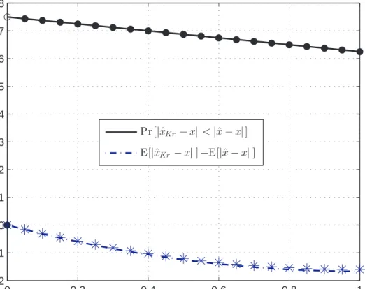
quasi-reflected individual and the solution of an optimization prob-lem, and the EA individual and that solution. . . 35 8 Distance and probability of being closer to solution forxˆKrandxˆ 39
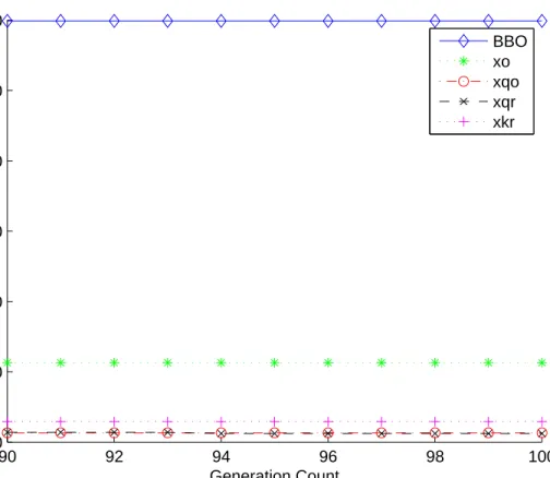
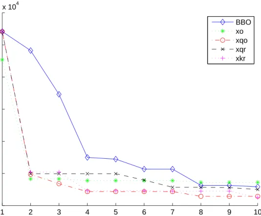
9 Fist ten generations of best results obtained for Colville . . . 48 10 Generations 90-100 of best results obtained for Colville . . . . 49 11 Fist 10 generations of best results obtained for Schwefel 1.2s. 51
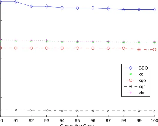
12 Generations 90-100 of best results obtained for Schwefel 1.2s 52
13 8-city closed path problem where the path is represented as a circle. . . 72 14 8-city closed path problem with opposite cities indicated across
the circular path. . . 73 15 Example of a three-color map . . . 78 16 Effects of dimension on the probabilities of various opposition
17 Model for cooperative coevolution . . . 93
18 An archipelago of seven islands connected with wheel rim topology as discussed in [215]. Each island represents a solver: differential evolution, simulated annealing or subplex. The islands are fully and bi-directionally connected. . . 95
19 Solution domain ifx∈[a,xˆ] . . . 98 20 Solution domain ifx∈[ˆx, c] . . . 98 21 Solution domain ifx∈[c,xˆo] . . . 99 22 Integration region of2x−xˆo<xˆqo < x . . . 100 23 Solution domain ifx∈[ˆxo, b] . . . 101 24 xˆqr solution domain . . . 102 25 Solution domain ifx∈[a,xˆ] . . . 103 26 Solution domain ifx∈[ˆx, c] . . . 103 27 Solution domain ifx∈[c,xˆo] . . . 103 28 Integration region of2x−xˆo<xˆqr . . . 104 29 xˆqr solution domain,x∈[ˆxo, b] . . . 105 30 Solution domain ifx∈[a,xˆ] . . . 106 31 Solution domain ifx∈[ˆx,xˆ+2c] . . . 106 32 Integration region ofxˆqo <2x−xˆ . . . 107 33 Solution domain ifx∈[a,xˆ] . . . 109 34 Solution domain ifx∈[ˆx, c] . . . 110 35 Domain ofxˆKr as a function ofK . . . 112 36 Solution domain ifx∈[a,xˆ] . . . 112 37 Solution domain ifx∈[ˆx, c] . . . 113 38 Solution domain ifx∈[c,xˆo] . . . 116 39 Solution domain ifx∈[ˆxo, b] . . . 117 40 Distribution ofxin domain [−b, b]. . . 119 41 Distribution ofxˆin domain [−b,0]. . . 119 42 Distribution of xˆ in domain [a, b] where K is the reflection
43 fˆxKr(z+y)in domain[a, b]whereK is the reflection weight. . 120
44 fˆxKr−x(y) . . . 121
45 Convolution of fxˆKrand fx. . . 121
46 Convolution of fxˆKrand fx. Shifting at the end points . . . 122
47 Convolution of fxˆKrand fx. Aszis increased, fxˆKr(z+y)is over-lapping fx(y) . . . 123
48 Convolution of fxˆKrand fx. fxˆ(z+y) is enclosed in fxˆ(y)as z is increased . . . 123
49 Convolution of fˆxKrand fx. fxˆ(z+y)starts shifting out of fx(y) asz is increased . . . 124
50 f|Z|(z) . . . 125
51 fˆx−x(y)can be obtained by convolving fxˆand fxaszshifts from [−b, b] . . . 126
52 Convolution of fxˆand fx. . . 126
53 Convolution of fxˆKrand fx. Shifting at the end points . . . 127
54 Convolution of fˆxand fx. Asz is increased, fxˆ(z+y)is overlap-ping fx(y) . . . 127
55 Convolution of fxˆKrand fx. Shifting at the end points . . . 128
56 Convolution of fˆxand fx. fˆx(z+y)starts shifting out of fx(y)as z is increased. . . 128
57 f|Z|(z) . . . 129
58 Two dimensional plot of the Beale Function . . . 132
59 Two dimensional plot of the DeJong F5 function . . . 134
60 Two dimensional plot of the Easom function . . . 135
61 Two dimensional plot of the Perm function . . . 136
62 Two dimensional plot of the Tripod function . . . 137
63 Two dimensional plot of the Ackley function . . . 138
64 Two dimensional plot of the Alpine function . . . 139
65 Two dimensional plot of the Fletcher function . . . 141
67 Two dimensional plot of the Penalty 1 function. . . 143
68 Two dimensional plot of the Penalty 2 function . . . 144
69 Two dimensional plot of the Quartic function. . . 145
70 Two dimensional plot of the Rastrigin function. . . 146
71 Two dimensional plot of the Rosenbrock function. . . 147
72 Two dimensional plot of the Schwefel 1.2 function. . . 148
73 Two dimensional plot of the Schwefel 2.21 function. . . 149
74 Two dimensional plot of the Schwefel 2.22 function. . . 150
75 Two dimensional plot of the Schwefel 2.26 function. . . 151
76 Two dimensional plot of the Sphere function. . . 152
77 Two dimensional plot of the Step function . . . 153
CHAPTER I
INTRODUCTION
M
ANY engineering problems involve nonlinearities or other complexities which render mathematical methods and even local optimization al-gorithms futile. However, nature has become an expert in “optimizing" dif-ficult, convoluted problems through evolution. Evolutionary computing (EC) attempts to replicate nature’s success by representing solutions as encoded in-dividuals and allows them to evolve through a selection mechanism. Where mathematics can guide toward a unique solution, solutions provided by nature are diverse. For instance, deer are known to have 34 species and many more subspecies. This variety, represented by their coats, size or antlers, enables them to adopt to various diets, predators and landscapes. While a white-tail deer hides and sprints away from predators, mule deer pronks away by jump-ing usjump-ing all four feet. Similarly, EC allows global minimization by creatjump-ing a population of solutions that are robust and adaptive. These solutions may not be perfectly optimal but they are evolved to be suitably fit solutions to the optimization problem. As stated by an anonymous quote “Perfection would be a fatal flaw for evolution. Life’s hold on life depends on God losing his grip on life every once in a while."in-troduces evolutionary computation, presents its history and common applica-tions. Section 1.2 gives an overview of biogeography-based optimization as an evolutionary algorithm and Section 1.3 discusses opposition as a tool for opti-mization. Section 1.4 lists the pseudo code for oppositional biogeography-based optimization. The motivation for this research is discussed in Section 1.5 and the problem statement is broached in Section 1.6.
1.1
Evolutionary Computation
Evolutionary computation is an umbrella term, that is, a hypernym, con-ceived in 1991 [1] to unite the various evolutionary techniques that were being simultaneously developed around the world. This section will discuss the de-velopment of EC, present an overview of its methodology, explore some contro-versies in academia (namely the No Free Lunch Theorem) and its applications as reported in today’s literature.
1.1.1
History of Evolutionary Computation
The evolution of evolutionary computation can be summarized as follows.
• Evolutionary simulations:
– 1954: The first implementation of EC is commonly credited to Bari-celli [2], who modeled cells migrating in a grid and competing for survival.
– 1958: On the opposite corner of the world, in Australia, another re-searcher [3] modeled sexual reproduction by recombining solutions.
• Evolutionary algorithms:
In Artificial Intelligence through Simulated Evolution, he explains [5]:
Intelligent behavior is a composite ability to predict one’s en-vironment coupled with a translation of each prediction into a suitable response in light of some objective.
EP relies solely on mutation for reproduction, not on recombination, and applies tournament style selection based on fitness. Also, unlike most other EAs, EP enables population size to evolve.
– In 1962, Holland published an article outlining a theory of adaptive systems [6]. Later, he published Adaptation in Natural and Artifi-cial Systems [7] which was instrumental in the development of ge-netic algorithms (GA). In GA, solution candidates were represented as chromosomes in a DNA in binary code and evolved by single point crossover and mutation. Holland’s GA gained popularity in part due to his Schema Theorem [8], also referred as the Fundamental The-orem of Genetic Algorithms: “Short, low-order schemata with above average fitness increase exponentially in successive generations." – 1964: Evolution strategies (ES) [9, 10] was designed by three
stu-dents as an automatic parameter selection algorithm for a laboratory experiment to minimize the drag in wind tunnel [11]. During the la-borious experiment, researchers discovered that heuristic search out-performed a discrete gradient-oriented method. They applied their algorithm to 2D and 3D air flow [12] and 3D hot water nozzle prob-lems [13]. Their proposed “cybernetic solution path" algorithm had two rules [14, 15]:
∗ Mutation: “Change all variables at a time, mostly slightly and at random."
∗ Survival of the fittest: “If the new set of variables does not di-minish the goodness of the device, keep it, otherwise return to
the old status."
• Swarm intelligence:
– Ant colony optimization was first published as Dorigo’s PhD disser-tation in 1992 [16]. He was inspired by the probabilistic behavior of ants [17] and specially the double bridge experiment [18]. In this ex-periment, a colony of ants must cross back and forth one of the two bridges to collect food from the other side. In time, ants converge to the shorter path by following the concentration of pheromone left behind by the previous colonists. Goss et al. [18] also proposed a mathematical model for the probability of an ant choosing a bridge based on the previously made decisions by the ants.
– 1995: Particle swarm optimization [19, 20] is a swarm intelligence method [21] that is based on the models of bird flocking [22]. It was originally designed to model social behavior where subjects altered their perspectives to better fit in with their peers. It has later been simplified to a heuristic optimization algorithm where each particle’s velocity determines its position based on information received from its neighborhood.
• Miscellaneous EC methods:
– Differential evolution (DE) is developed by Storn in 1995 [23, 24] and is considered to be a robust EA for avoiding premature convergence found in GA [25, 26]. In DE, an individual is created based on the weighted difference of two other solution candidates added to a third random solution candidate [27]. If this new individual is more fit than an individual randomly selected from the current generation, it replaces that individual. Performance of DE depends on the
se-evaluations.
– Genetic programming (GP) is born in 1985 when Cramer created an algorithm that develops simple sequential programs [29]. He uti-lized GA to manipulate tree-like structures that represented ran-domly generated functions. His work was later expanded by Koza to evolve more complicated programs [30, 31, 32]. GP has evolved from being solely a program creator. It is also a popular method for automatic circuit design where given a set of requirements, GP gen-erates the desired circuit routing, placement and size [33, 34].
– Simulated annealing (SA) is independently developed by two scien-tists in the mid-1980s [35, 36] and is a generalization of the Metropolis-Hastings algorithm (MH) [37]. MH is a Monte Carlo method that allows sampling from a probability distribution and only requires density function evaluation. Annealing is the process of heating a thermodynamic system and then slowly cooling it. The goal of SA is to minimize the system’s energy by moving from current states to a neighboring state based on an acceptance probability function which depends on states’ energies and a global decay parameter that repre-sents the temperature. SA began as an optimizer for combinatorial problems [35, 38, 39] and its variations include quantum annealing [40] and stochastic tunneling [41].
– Tabu search (TS), published by Grover in 1985 [42, 43, 44], explores the neighborhood of an individual in search of a more fit solution while remembering a list of recently visited neighbors, marked as taboo, to avoid revisiting them. Therefore, if the algorithm is stuck in a local minima, instead of retreating, it is forced to explore in a new direction. TS can solve combinatorial problems including graph coloring [45, 46, 47].
1.1.2
Evolutionary Computation Methodology
Biomimicry, drawing inspiration from nature for developing new tech-nology, is now employed in many scientific fields. Recently, NBD Nano has designed a water bottle that refills itself by extracting moisture from the air [48]. This technology imitates the Namib Desert beetle’s wings’ coating which catches the water from the morning fog. However, this is not the first exam-ple of biomimicry. In the fifteen century, Leonardo Da Vinci studied birds’ anatomy to design his flying machine [49]. Many of today’s inventions, from Velcro to nose of Shinkansen (Japan’s bullet train), mimic solutions from ture [50]. Universities and corporations have started research centers for na-ture inspired funa-ture development ideas [51, 52]. As seen by EC’s history, many evolutionary algorithms and other machine intelligence learning methods are also inspired by nature. For example, genetic algorithms (GA) [8] mimic evo-lution, ant colony optimization (ACO) [16] approximates animal behavior in colonies, and artificial neural networks [53] are modeled after the biological nervous system. Other examples include particle swarm optimization [19], ar-tificial immune systems [54] and hill climbing [55]. The majority of these EAs follow a similar methodology which could be outlined as:
• Initialize population
• Selection
• Recombination
• Random variation
Generally, the process starts by creating an initial random population of possible solutions. The population is then processed in a way which is moti-vated by the natural model. Based on this natural model’s properties, such as genetic inheritance and survival of the fittest, the population will evolve and
each generation. The algorithms generally quit once an acceptable solution is found or when the available computing resources are exhausted.
1.1.3
Controversies and No Free Lunch Theorem
One of the benefits that made EC popular is that it can be applied to var-ious types of problems. However, generally, EAs are not modified to match the cost functions of the problem at hand and the same search algorithm is used regardless of a problem’s particulars. Reference [56] shows that the differences in cost functions are crucial. The authors prove that when we ignore the par-ticular biases or properties of a cost function, the expected performance of all algorithms over all cost functions is precisely identical. This is called the No Free Lunch Theorem (NFL).
Their main theorem is that the probability of obtaining a particular his-togram of cost values given a specific number of cost evaluations is independent of the algorithm used given that we have no prior information about the opti-mization problem. This implies that if we have no prior knowledge about the cost function, the expected performance will be independent of the chosen algo-rithm. The theorem relies on the assumption that since nothing is known about the cost functions, then, on average, all cost functions have the same probabil-ity distribution. They further conclude that the expected distribution of the histogram will be the same regardless of the selected algorithm. Therefore, the EA should be chosen based on the distribution of the cost function.
The theorem is named No Free Lunch Theorem (NFL) and is applied to search [56], supervised learning [57, 58] and optimization [59]. Further development lists the necessary conditions for NFL [60, 61]. NFL theorem created controversy about the credibility of EC [62, 63]. However, not everyone agrees with NFL’s applicability to real-world problems. Reference [64] disputes the validity of the NFL in black box scenarios and proposes the Almost No Free Lunch Theorem.
1.1.4
Evolutionary Computation Applications
EC has been used to assist in solving countless problems in a variety of fields from geophysics to financial markets. This section will discuss some of this research. In aerospace engineering, EC has been applied to wing shape design of an aircraft [65, 66] and maneuvers of a spacecraft while minimizing time [67, 68]. In chemistry, it has been used in the design of new molecules to meet given set of specifications [69] and creating new antimicrobial com-pounds for cleaners [70]. Another area where EC is applied is control systems. It has been employed in online controller design [71] and many offline ones including linear quadratic-Gaussian and H∞ control [72, 73, 74], as well as control of chemical reactors [75, 76]. EC has been utilized for motion planning in robotics [77, 78, 79, 80] and network design in communications [81, 82, 83]. In finance, EC has been employed for bankruptcy [84, 85, 86] and stock predic-tions [87, 88, 89]. In geophysics, EC has been applied to seismic wave inversion [90, 91, 92] and groundwater monitoring [93, 94]. Holland and Miller draw a parallel between economic systems and complex adaptive systems and employ artificial adaptive agents to predict economic phenomena [95]. Another popular application is protein building and folding simulations in biology [96, 97, 98]. Reference [99] develops fuzzy rules tuned by EA for linguistic modeling. This list can be expanded to add materials science, law enforcement, data mining and countless other fields. As one can see, EC has been improving our lives in various fields, no less than any other established science. One can expect it to have even more applications in the future as the theory behind it is further developed and as computing power continues to become cheaper.
1.2
Biogeography-based Optimization
biogeogra-That is, they sustain their own distinctive organisms and they are numerous. There are more islands than there are continents or oceans [100]. Due to the variations they provide (size, ecology, length and degree of isolation), islands can offer the necessary tools for studying evolution. Charles Darwin, credited as the formulator of the theory of evolution, conceived his hypotheses on nat-ural selection after studying/eating giant tortoises on the Galapagos Islands [101].
Seeing that biogeography helped the development of theory of evolution, it stands to reason that biogeography would be a solid candidate for evolu-tionary computation. Population biology studies the impact of immigration, emigration and extinction on the number of species. BBO is modeled after the immigration and emigration of species between islands. The fitness of each is-land is measured by its habitat suitability index, HSI [102]. A habitat with a high HSI indicates a desirable living environment in biogeography and a good solution in BBO. This type of habitat will host many species and spread its species frequently to other habitats. Because a high HSI island hosts a large number species, it will be harder to immigrate there and this type of solution will be less susceptible to alterations and therefore its HSI will remain more static throughout many generations.
On the other hand, a habitat with a low HSI will be hosting a limited number of species and these species will have a lesser chance of being accepted to other islands. It will be very easy for the species from other islands to mi-grate to low HSI habitats. Therefore, the species distribution on low HSI is-lands will change more frequently.
The independent variables of the HSI are called the suitability index variables (SIVs). SIVs are the climatic and topographic features offered by the island and can include such factors as precipitation, temperature, elevation and slope.
Fig. 1 illustrates linear BBO immigration and emigration curves. In this figure, the estimated solutions are sorted by fitness from worst to best. The
worst solution candidate, with a low HSI, has the highest immigration rate; hence, it has a very high chance of borrowing features from other solutions, helping it to improve for the next generation. The best solution candidate, with a high HSI, has a very low immigration rate, indicating that it is less likely to be altered by the other individuals. The emigration rate works in the opposite direction.
Worst Solution Best Solution
Migration rate
Solutions sorted by fitness
←λ, immigration rate
µ, emigration→ rate
Figure 1. Linear migration rates plotted against the sorted population. Better solu-tion candidates possess a low immigrasolu-tion rate and a high emigrasolu-tion rate.
BBO migration functions are programmed as described above. The other area of biogeography, extinction, is implemented indirectly. When fitter species immigrate to an island, lesser fit species must go extinct to accommodate the new ones. However, note that emigration in BBO does not symbolize a move, but rather a copy. For example, if a feature in island 1 migrates to island 2, then both islands 1 and 2 have this feature. The worst solution candidate is assumed to have the worst features; thus, it has a very low emigration rate and a low chance of sharing its features. On the other hand, the fittest solution candidate has the best features and the highest probability of sharing them.
and continues to survive. Also, when updating the population, BBO considers the fitness of the immigrating and emigrating islands via the emigration and immigration curves.
Mathematical modeling and convergence properties of EC are still being investigated as modeling the dynamics of an adaptive system is difficult. One approach to confirm convergence is to formulate the EA as a finite state Markov chain. While [103] derived the necessary conditions for asymptotic convergence to optimum for GA and ES, [104] proved their convergence. This proof is accom-plished by finding the limit of the probability of nearing the global optimum as the number of iterations goes to infinity. The proof illustrates that EA will be in a certain vicinity of the optimal point with a probability of 1. However, prac-ticality of this proof is rather limited in the real world as it assumes infinite time for convergence. Reference [105] extends this work to BBO and derives the limiting probabilities for all possible population distributions.
Despite being a new algorithm, BBO has already been implemented in many fields of engineering. It has been applied to the power flow problem [106, 107, 108, 109], economic dispatch [110, 111, 112], image classification [113, 114, 115], communications [116, 117, 118] and robotics [119, 120, 121]. While statistical foundations for BBO are being developed [122, 123], BBO has been combined with other EAs such as ES [124], DE [125], PSO [120], and flower pollination by artificial bees [126] to form hybrids. In addition, it has been utilized to optimize other EC methods, such as fuzzy [127] and neuro-fuzzy [128] systems.
1.3
Opposition-based Learning
In this section we discuss the numerous definitions of opposition in vari-ous areas of culture and science, and explain how it can be applied to optimiza-tion problems. Study of opposioptimiza-tion has been going on for millennia. The oppo-site forces have been studied by humanity for a long time on a philosophical
level. Dualities found in many religions are an example of this. Dualities have different interpretations in different cultures. In Taoism, yin-yang (shown in Fig. 2) reflects the harmony of opposite forces and seeks balance in complemen-tary forces. Two ancient Persian religions, Zoroastrianism and Manichaeism, are also considered dualistic. Manichaeism was one the most predominant re-ligions of its time, spreading from Roman Empire to China. In Manichaeism, dualism existed as a struggle between good and evil. As Manichaeism gained popularity, it was declared a heresy in Christianity, oppressed by Islam and forbidden in China by Ming dynasty.
What might have started as a theological debate (yin vs. yang and good vs. evil), still exists today in the scientific world. In electrical engineering, duality refers to the relationship between capacitance and impedance or open and short circuits. In mechanical engineering, duality indicates the relation-ships between stress and strain, stiffness and flexibility. In magnetism, the dual of magnetic field is the electric field and the dual of permittivity is perme-ability. Furthermore, in mathematics, duality is studied in logic, set and order theories.
Another example of opposition in today’s scientific world is the study of antimatter. Physicists believe that all particles have a mirror image in the universe, called antimatter. International groups of researchers at CERN are conducting the world’s most expensive science experiment to create such an-tiparticles. They believe that studying and experimenting with antimatter will allow them to test the doctrine of modern physics and standard model of par-ticle physics [129]. This research is so crucial to the field that based on its outcomes “the textbooks ... [may] have to be rewritten," according to Jeffrey Hangst from CERN [130]. Even though we do not fully understand antimat-ter, certain applications of it are seen in today’s technology (for example, in medicine, anti-electrons are used for tomography scanning).
Figure 2. Yin-yang representing the harmony of opposing forces in Eastern philoso-phy
Opposition is encountered in different fields under different names. In Euclidean geometry it is referred as inverse geometry, in physics it is the par-ity transformation and in mathematics, it denotes reflection. All of these def-initions involve isometric self-mapping of a function. Other examples include astronomy where planets that are 180◦ apart are considered to be opposing each other. Opposites also have a significant meaning in semantics as general-ization of antonyms. Where antonyms are limited to gradable terms, such as thin and thick, the term opposite can be applied to gradable, non-gradable and pesudo-opposite terms.
The idea of OB B O is derived from opposition-based learning (OBL). The creators of the OBL believe that a shortcoming of natural learning is that it is time consuming since it is modeled after a very slow process. For instance, it requires countless life cycles for species to evolve. On the other hand, human society progresses at a much faster rate via “social revolutions." Hence, the learning process could be improved based on such a model. Describing revolu-tions as fast and fundamental changes, whether in politics, economics or any other context, Tizhoosh maps this theory to machine learning and proposes to use opposite numbers instead of random ones to quickly evolve the population [131].
the solution. The inventors of OBL advocate that given a random number, generally, its opposite has a higher chance of being closer to the solution than a random point in the search space. Thus, by comparing a number to its opposite, a smaller search space is needed to converge to the right solution(s). In this research, we develop the proofs measuring the effectiveness of opposite points against random numbers.
OBL has its roots in reinforcement learning [132, 133] and has been ap-plied to various soft computing methods such as neural networks [134, 135, 136, 137] and fuzzy systems [138, 139]. To date, OBL has been employed to accelerate the convergence properties of numerous evolutionary algorithms such as differential evolution [140, 141, 142, 143], particle swarm optimization [144, 145, 146, 147], ant colony optimization [148, 149] and simulated anneal-ing [150] in a wide range of fields from image processanneal-ing [151, 152, 139] to system identification [153, 154].
The algorithm is implemented as two functions. The first one is called only once per simulation during initialization to create the initial population. This function compares the initial random population and its opposite to select the most fit among them. The second function is called every Jr generations,
where Jr, jumping rate, is a control parameter set by the user to jump, or
skip, opposite population creation at certain generations. Since the opposition function is called twice, OB B O is classified as an “initializing and somatic ex-plicit opposition-based computing algorithm" [155]. Because the opposite pop-ulation’s fitness has to be evaluated, OB B O will have to converge faster than original BBO (in terms of generation count) in order to maintain the same CPU load. A benchmark method based on number of cost function calls is introduced in Section 3.1 to take this into consideration.
1.4
Algorithms
In this section, we provide an outline of the main function which eval-uates the EA and opposition algorithms, as well a brief overview of each EA. Whether we employ GA, DE or BBO as the optimization algorithm, Algorithm 1 is used to seek for the global minimum.
Algorithm 1 Pseudocode for EA with opposition where rand ∈ [0,1] is a uni-form random number
1: Main EA Function
2: Create an initial random population
3: Replace duplicate individuals with random ones 4: Calculate the cost of each individual
5: Sort the population
6: Execute the opposition algorithm (Algorithm 2)
7: while Optimal solution is not found or cost evaluation limit is not reached do
8: Perform EA selection/recombination (Algorithms 4−6) 9: Replace duplicate individuals with random ones
10: Ensure that each individual is valid
11: Calculate the cost of the updated individuals 12: Sort the population
13: if rand≤opposition jumping ratethen
14: Execute the opposition algorithm (Algorithm 2) 15: end if
16: Apply elitism by replacing the worst of current generation with the best of the previous generation
17: Ensure that each individual is valid 18: Sort the population
19: end while
or BBO which are described in following subsections and Algorithms 4, 5 and 6. Line14calls the opposition opposition function as outlined in Algorithm 2. Algorithm 2 Pseudocode for opposition logic
1: Opposition Function
2: Create an opposite population,xˆo,xˆqo,xˆqrorxˆKr, as defined in Chapter II
3: Calculate the cost of each opposite individual
4: Select the fittest individuals amongst the EA and opposite populations 5: return F ittest Individuals
1.4.1
Genetic Algorithms
GA is one of the most popular EA and many variations of it exist in the literature [156]. We employ GA with uniform crossover and roulette-wheel selection as described in Algorithms 3, 4. The probability of selection with roulette wheel is directly proportional to each individual’s fitness. The crossover rate is set to 50%; thus, on average, each child will have half of each parent’s genes.
Algorithm 3 Pseudocode for roulette-wheel selection of parents 1: Roulette-Wheel Function
2: Cumulative sum of all costs, Σc
3: Running sum, Σs = 0
4: for Each Solution Candidate,S do 5: Σs = Σs+Cost(S)/Σc
6: ifrand(0,1)<Σs then
7: Parenti =S
8: end if 9: end for
Algorithm 4 Pseudocode for one generation of genetic algorithm function 1: GA Function
2: Select parents using roulette-wheel (Algorithm 3) 3: Produce children:
4: for Each Pair of Parents,P1 andP2 do
5: for Each Problem Dimension,ddo 6: ifrand(0,1)<Crossover ratethen 7: C1d=P1d 8: C2d=P2d 9: else 10: C1d=P2d 11: C2d=P1d 12: end if 13: end for
14: Form two new solution candidates from children 15: end for
16: Mutation:
17: for Each Solution Candidate,S do 18: for Each Problem Dimension,ddo 19: ifrand(0,1)<Mutation ratethen 20: Sd=rand(mind, maxd)
21: end if
22: end for 23: end for
1.4.2
Differential evolution
While most EA’s start with recombination, DE begins each generation with mutation operation by creating the donor vector:
v =r1+F(r2−r3) (1.1)
where r1, r2 and r3 are randomly selected, distinct solution candidates and F is the weighting factor. Then, based on the crossover probability, CR, a trial vector,ud, is formed from the donor vector and the current solution candidate,
Sd: ud= vd if rand(0,1)≤CRORd=rand(1, D) Sd otherwise (1.2)
where d is the independent variable and D is the problem dimension. The
rand function returns a uniformly distributed random integer within the given closed interval. The logical OR statement ensures that at least one variable is taken from the donor vector while forming the trial vector. Finally, if the trial vector is fitter than the the current solution candidate, the trial vector replaces it in the next generation. This flavor of the DE algorithm is commonly referred as DE/rand/1/bin [157] and is outlined in Algorithm 5.
Algorithm 5 Pseudocode for one iteration of differential evolution function 1: DE Function
2: for Each Solution Candidate,S do
3: Select 3 unique individuals from the population: r1, r2, r3
4: Form the donor vector, v: 5: v =r1+F(r2−r3)
6: for Each Problem Dimension,ddo 7: Form the trial vector,u:
8: ifrand(0,1)≤CRORd=rand(1, D) then
9: ud=vd
10: else
11: ud=Sd
12: end if
13: end for
14: The fitter of the two survives: 15: ifCost(u)≤Cost(S)then
16: S′ =u 17: else 18: S′ =S 19: end if 20: end for 21: S′ =S
22: return Best Individual
1.4.3
Biogeography-based Optimization
For this research, we implement partial immigration-based BBO as de-scribed in [122]. Partial immigration indicates that the initial selection of is-lands is based on immigration rates, λ, and emigration decisions are made at the level of each independent variable via roulette wheel selection. BBO’s re-production scheme is named blended migration as proposed in [158]. Blended
migration is based on blended crossover which was developed for genetic algo-rithms [159]. Blending refers to the act of combining the reproducing individu-als using a blending parameter,α. The BBO migration scheme is presented in Algorithm 6.
Algorithm 6Pseudocode for one iteration of biogeography-based optimization function.
1: BBO Function
2: Assign immigration rates: λi ∝ranki
3: Assign emigration rates: µi = 1−λi
4: for Each Solution Candidate,Si do
5: for Each Problem Dimension,ddo 6: Select immigrating feature Si,d ∝λi
7: Select emigrating featureSj,d ∝µj
8: Si,d =αSi,d+ (1−α)Sj,d
9: end for 10: end for
11: Perform Mutation:
12: for Each Solution Candidate,S do 13: for Each Problem Dimension,ddo 14: ifrand(0,1)<Mutation ratethen 15: Sd=rand(min, max)
16: end if
17: end for 18: end for
19: return Best Individual
difficult problems yields promising results; however, there is still a need for development in EAs, especially in mathematical understanding. Based on the presented literature review, we see the following lack.
• Opposition theory has already been proposed for solving continuous time optimization problems. However, there is a need for analyzing the ef-fectiveness of choosing opposition over random numbers. Therefore, in Chapter II and Section 2, we study the statistical properties of opposition for heuristic optimization algorithms.
• The statistical analysis yield to the proposal of new oppositional algo-rithms. Mathematical analysis of the proposed algorithms are presented in Chapter II and Sections 3-4. The validity of these novel methods is fur-thered analyzed in Chapter III with the help of real-world and benchmark problems.
• Many manufacturing and combinatorial problems are defined in discrete domain. However, the current definition of opposition is not valid for these type of problems. Therefore, in Chapter IV , we extend opposition to discrete domain problems.
1.6
Contributions of This Research
BBO is a newer evolutionary algorithm, but it already has proven it-self a worthy competitor to the better known EAs, such as genetic algorithms, differential evolution, and ant colony optimization. BBO is a great way to ap-proach complex nonlinear problems because it can outperform or match other EAs with less computational effort. However, there is still some room left for improving BBO since many other techniques exist in the literature that are utilized to enhance other EAs. Our goal is to experiment with these algorithms and adapt them to BBO to demonstrate BBO’s highest potential. In order to achieve this goal, we introduce quasi-reflection as a new opposition method
and mathematically prove that it yields the highest expected probability of be-ing closer to the solution among all OBL methods.
In this research, probabilistic analysis of OBL is introduced in Chapter II where we mathematically compare all existing opposition techniques and in-troduce a novel opposition method that is mathematically proven to be better than previous methods. Chapter III presents the results of our empirical analy-sis comparing the existing and new oppositional algorithms. The performance of the algorithms are tested on low and variational dimensional benchmark problems taken from the literature and real-world space trajectory optimiza-tion problems provided by European Space Agency. The significance of our findings are also discussed by employing statistical tests. Chapter IV extends opposition to discrete domain optimization problems. Chapter V discusses fu-ture work and presents concluding remarks. The detailed mathematical proofs for the results presented in Chapter II are given in Appendix A. Appendix B defines the low and variable dimensional benchmark functions and Appendix C lists the publications resulted from this research.
CHAPTER II
PROBABILISTIC ANALYSIS OF
OPPOSITION-BASED LEARNING
T
HIS chapter presents up-to-date definitions of the opposition methods as reported in the literature and introduces new ones. We statistically com-pare existing and new oppositional techniques in one-dimensional space. Sec-tion 2.1 presents the definiSec-tions of various opposiSec-tional points. SecSec-tion 2.2 derives the proofs of how often the quasi-opposite and reflected points are closer to the solution of an optimization problem than an EA individual or its opposite. Section 2.3 introduces a new, fitness-dependent quasi-reflection method and proves how often this new variable is closer to the solution than an EA individual. Section 2.4 derives the expected distance between the fitness-dependent quasi-reflection method and the optimal solution. Finally, Section 2.5 summarizes the proofs derived in the chapter.2.1
Definitions of Oppositional Points
In [142], Rahnamayan introduced quasi-opposition-based learning and proved that a quasi-opposite point is more likely to be closer to the solution of
the optimization problem than the opposite point. In this section, we extend on this proof to show how much a quasi-opposite point is better than an opposite point. First, let us define opposite and quasi-opposite numbers in one dimen-sional space. These definitions can easily be extended to higher dimensions. Definition Letxˆbe any real number∈[a, b]. Its opposite,xˆo, is defined as
ˆ
xo =a+b−xˆ (2.1)
Notice that similar definitions already exist in mathematics. In Euclidean ge-ometry, the opposite is referred as the inversion of point x. In addition, if the center of the domain is 0, then the opposite can be simplified as the additive inverse where −x is the additive inverse of x. In Euclidean space, inversive geometry studies other such transformations such as circle and curve inver-sion. Since after these transformations, the distance is preserved, opposition as defined in Eq. (2.1) can be described as an isometric mapping.
Definition Let xˆ be any real number ∈ [a, b]. Its quasi-opposite point, xˆqo, is
defined as follows [131]:
ˆ
xqo =rand(c,xˆo) (2.2)
wherecis the center of the interval[a, b]and can be calculated as(a+b)/2, and rand(c,xˆo) is a random number uniformly distributed betweencandxˆo.
Note that unlike opposition, the quasi transformation is not a linear transfor-mation because it involves the random function. It is also not an isometric transformation since the quasi-opposite point is not always placed equally far from the reflection point.
Since we reflect xˆ to obtain xˆo to accelerate the EA exploration process,
we propose to apply the same logic and reflect the quasi-opposite point, xˆqo, to
obtain the quasi-reflected point,xˆqr.
where rand(c,xˆ) is a random number uniformly distributed betweencandxˆ.
If x is the unknown solution to an optimization problem and xˆ is an in-dividual in an EA, then xˆo is the opposite of the EA individual and xˆqo and
ˆ
xqr are the quasi-opposite and quasi-reflected individuals, respectively. Fig. 3
illustrates a point xˆ, its opposition, xˆo, its quasi-opposition, xˆqo and its
quasi-reflection, xˆqr as defined in Eqs. 2.1-2.3. Earlier we discussed that opposition
has different meanings in different fields. We can interpret the opposite points defined in Fig. 3 with an example from semantics. Letxˆbe the statement that “Jane is short"; then the opposite statement, xˆo would be “Jane is not short"
or “Jane is tall". The quasi definitions are more fuzzy. xˆqo would indicate that
“Jane is taller than most" and xˆqr would mean the opposite of xˆqo: “Jane is
shorter than most". This explanation is comparable to a fuzzy membership degree from fuzzy set theory. Also, it is analogous to the categorization of oppo-sition in the Aristotelian logic where the square of oppooppo-sition (Fig. 4) illustrates the relationship among the contradictory propositions.
a xˆ c xˆo b
ˆ xqr
z }| {z xˆ}|qo {
Figure 3. Opposite points defined in domain[a, b]. c is the center of the domain and
ˆ
x is an EA individual. xˆo is the opposite of xˆ, and xˆqo and xˆqr are the
!"#$%&%'(%)%* +,'!"#()-%.//'#0)1'!" 23%&%'(%)%* +,'!"#()-%,"4)1'!" &30"%&%'(%* *)#1'56-)#%)//'#0)1'!" &30"%&%'(%,31%* *)#1'56-)#%,"4)1'!" 53,1#)#'"( (67)-1 "#,( (67)-1 "#,( (6753,1#)#'"( 53,1#)8'513#'"(
Figure 4. Square of opposition, conceived by Aristotle, classifies the relationships be-tween opposing propositions [155].
Notice that in Fig. 3, the degree of opposition increases as we move fur-ther away fromxˆ. The term degree of oppostion is defined in [155] and a crude proposal for quantifying the level of opposition is presented in Table I. We can say that in OBL, points with a higher degree of opposition dominate over the lesser degrees. Super opposition, xˆs, is defined in [155] as all points between
[a, b]exceptxˆ, therefore it is a superset of all defined opposite points and more. For the semantic example given above,xˆswould include the statement “Jane is
the shortest" as well as “Jane is the tallest". Super opposition is not discussed any further in this research.
Table I.Assignment of opposition degrees to the defined opposite points based on the opposition distance from the reflected point.
Degree of opposition Opposition method
0 Solution estimate,xˆ
1 Quasi-reflection,xˆqr
2 Quasi-opposition,xˆqo
3 Opposition,xˆo
4 Super opposition, xˆs
2.2
Probabilistic Overview of Opposition
This section will derive the following expected probabilities, where x is the unknown solution to an optimization problem, xˆ is an EA candidate solu-tion, and the expected value is taken over the probability density functions of xandxˆ.
• Pr [|xˆqo−x|<|xˆo−x|]: In Theorem 2.2.1, we prove how likely it is that a
quasi-opposite point is closer than the opposite of an EA individual to the solution of an optimization problem.
• Pr [|xˆqr−x|<|xˆo−x|]: In Theorem 2.2.2, we prove how likely it is that a
quasi-reflected point is closer than the opposite of an EA individual to the solution of an optimization problem.
• Pr [|xˆqo−x|<|xˆ−x|]: In Theorem 2.2.3, we prove how likely it is that a
quasi-opposite point is closer than an EA individual to the solution of an optimization problem.
• Pr [|xˆqr−x|<|xˆ−x|]: In Theorem 2.2.4, we prove how likely it is that a
quasi-reflected point is closer than an EA individual to the solution of an optimization problem.
We should note that all our proofs are in one dimensional space and we assume that the solutionxof the optimization problem has a uniform distribution.
Our assumption of uniformity is validated by the Principle of Insufficient Reason proposed by Bernoulli [161] and Laplace [162], although neither math-ematician named the principle. The name is given by the critics of the theorem as a wordplay of Leibnitz’s Principle of Sufficient Reason [163] which states that “nothing happens without a reason". According to the Principle of Insuffi-cient Reason, “in the absence of prior knowledge, we must assume that events Ai have equal probabilities" [164]. As an example, one can consider tossing a
coin. Probabilities of obtaining a head or a tail are assumed to be equal because we presume that the probability of occurrence of one over the other is unlikely. Another example would be picking a card from a deck. Since we don’t have any knowledge of the distribution of the cards in the deck, we assume that all cards have equal probability of being picked.
Finally, we assume that the problem domain is symmetric about 0, thus b = −a. This assumption is made for ease of notation, and can be relaxed without losing the generality of the results.
Theorem 2.2.1. Assume that the solution xof an optimization problem is uni-formly distributed in a one-dimensional search space. Then the probability av-eraged over allxand allxˆthat a quasi-opposite pointxˆqois closer to the solution
than the opposite of an EA individualxˆo is11/16.
Proof. See Appendix A.1.
Theorem 2.2.2. Assume that the solution xof an optimization problem is uni-formly distributed in a one-dimensional search space. Then the probability av-eraged over allxand allxˆthat a quasi-reflected pointxˆqris closer to the solution
than the oppositexˆo of an EA individual is9/16.
ary algorithm individual in more detail. First, we compute the probability of ˆ
xqo being closer than xˆ to the solution of an optimization problem, x, and the
expected value of this probability under certain conditions.
Theorem 2.2.3. Assume that the solution xof an optimization problem is uni-formly distributed in a one-dimensional search space. Then the probability av-eraged over allxand allxˆthat a quasi-opposite pointxˆqois closer to the solution
than an EA individual is9/16. Proof. See Appendix A.3.
The final lemma in this section is the probability ofxˆqrbeing closer than
ˆ
x to the solution of an optimization problem,x, and the expected value of this probability.
Theorem 2.2.4. Assume that the solution xof an optimization problem is uni-formly distributed in a one-dimensional search space. Then the probability av-eraged over allxand allxˆthat a quasi-reflected pointxˆqris closer to the solution
than an EA individual is11/16. Proof. See Appendix A.4.
2.3
Fitness-Weighted Quasi-Reflection
In this section, we introduce a new opposite point named fitness-dependent quasi-reflection or xˆKr. Unlike xˆqr, xˆKr is a not an independent random
vari-able. Instead, it is defined as the function of the fitness ofxˆ. This way we can control the amount of reflection based on the fitness of the individual. Thus, fit solutions can be reflected by a smaller amount than less fit solutions. xˆKris
defined as ˆ xKr = ˆ x+ (c−xˆ)K ifxˆ≤c c+ (ˆx−c)(1−K) ifx > cˆ (2.4)
whereK ∈(0,1]is the reflection weight and can further be described as:
K = Solution rank
Population size (2.5)
and solution rank = 1 for the best individual in the population.
Even though, fitness-dependent reflection is applied to xˆqr here, it can
easily be applied to any other opposition method. However, since xˆqris shown
to have the highest probability of being closer to the solution, it is taken as the base for thexˆKralgorithm.
Eq. 2.4 can be redefined by using the unit step function, U(x). The unit step function of x is a discontinuous function that is defined as 0for negative values ofxand 1for the remaining values ofx.
ˆ
xKr = [ˆx+ (c−xˆ)K]U(c−xˆ) + [c+ (ˆx−c)(1−K)]U(ˆx−c) (2.6)
ˆ
xKr eliminates the need for the previously defined random function by
considering the relative fitness of the individual. Let the center of the domain, c, be zero. Then Eq. 2.4 can be simplified as
ˆ
xKr = ˆx(1−K) (2.7)
This section derives results that are analogous to Theorem 2.2.4 for the fitness-weighted quasi-reflected point and computes the probability ofxˆKrbeing
closer than xˆ to the solution of an optimization problem, x, and the expected value of this probability as a function of the reflection weight,K.
Theorem 2.3.1. Assume that the solution of an optimization problem is uni-formly distributed in a one-dimensional search space. Then the probability av-eraged over allxand allxˆthat a fitness-weighted quasi-reflected point is closer than an EA individualxˆto the solutionxis(6−K)/8.
ranking among the population of solution candidates. Here, we would like to validate our findings for xˆKr by comparing it to those of xˆqr . Recall that in
Theorem 2.2.1, we obtained
Pr [|xˆqr−x|<|xˆ−x|] =
11
16 (2.8)
In this section, when we definedxˆKr = ˆx−Kxˆ, we proved that
Pr [|xˆKr−x|<|xˆ−x|] =
6−K
8 (2.9)
for K ∈ (0,1]. If we assume that K, the reflection weight, is uniformly dis-tributed, then E[K] = 12 and the expected value of Eq. 2.9 becomes equal to Eq. 2.8: EK{Pr [|xˆKr−x|<|xˆ−x|]}=EK { 6−K 8 } = 11 16 (2.10)
where EK indicates calculating the expected value with respect toK.
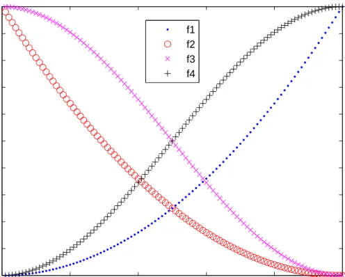
Further-more, K can be designed to have a non-uniform distribution so different re-flection patterns can be developed to better fit a given problem. Equation 2.5 defines the reflection weight as a linear function of individual fitness. How-ever, based on our expertise on a given problem, we can choose different K values. Table II lists four complementary functions, quadratic and sinusoidal, that could be used to create the reflection weights. Plots of these nonlinear functions are presented in Fig. 5. These functions are inspired from the BBO migration models presented in [165].
Table II.Example of quadratic and sinusoidal functions that can be used to create reflection weights wherer is the rank of an individual, where 1 is best, andpis the population size.
Label Reflection weight f1 ( r p )2 f2 (r p −1 )2 f3 1 2 ( cos ( rπ p ) + 1 ) f4 1 2 ( −cos ( rπ p ) + 1 )
0 20 40 60 80 100 0 0.1 0.2 0.3 0.4 0.5 0.6 0.7 0.8 0.9 1 Percentile Rank K f1 f2 f3 f4
Figure 5. Four possible nonlinear reflection weights based on individual rankings.
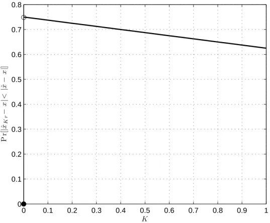
Fig. 6 plots the expected probability of xˆKr being closer than xˆto the
solution as a function of reflection weight. The results are derived theoretically and verified via simulation. Note that there is a discontinuity in Fig. 6 when K = 0, where the probability is 0. After this point, at K = 0+, the probability jumps to about 75%.
0 0.1 0.2 0.3 0.4 0.5 0.6 0.7 0.8 0.9 1 0 0.1 0.2 0.3 0.4 0.5 0.6 0.7 0.8 P r[ | ˆ xK r − x | < | ˆ x − x | ] K
Figure 6. Expected probability that xˆKr is closer to the solution of an optimization
problem than an EA individual
2.4
Distance Between a Fitness-Dependent
Quasi-Reflected Point and the Solution
In Section 2.2, we compared the probability ofxˆqr being closer than xˆto
the optimal solution x. Later, in Section 2.3 we defined xˆKr to be a
fitness-weighted quasi-reflection point that is a function of the reflection weight K and xˆ. We then calculated the expected probability of xˆKr being closer than
ˆ
xto the optimal solution x as a function of the reflection weight K. In this section, we calculatexˆKr’s distance to the optimal solution as a function of the
reflection weightK andxˆ. Recall that
ˆ
![Figure 4. Square of opposition, conceived by Aristotle, classifies the relationships be- be-tween opposing propositions [155].](https://thumb-us.123doks.com/thumbv2/123dok_us/1366882.2683019/45.918.212.769.166.536/figure-opposition-conceived-aristotle-classifies-relationships-opposing-propositions.webp)