SemEval 2016 Task 11: Complex Word Identification

SemEval 2016 Task 11: Complex Word Identification

Gustavo Henrique Paetzold and Lucia Specia

Department of Computer Science University of Sheffield, UK

{ghpaetzold1,l.specia_}@sheffield.ac.uk

Abstract

We report the findings of the Complex Word Identification task of SemEval 2016. To cre-ate a dataset, we conduct a user study with 400 non-native English speakers, and find that complex words tend to be rarer, less ambigu-ous and shorter. A total of 42 systems were submitted from 21 distinct teams, and nine baselines were provided. The results high-light the effectiveness of Decision Trees and Ensemble methods for the task, but ultimately reveal that word frequencies remain the most reliable predictor of word complexity.

1 Introduction

Complex Word Identification (CWI) is the task of deciding which words should be simplified in a given text. It is commonly connected with the task of Lexical Simplification (LS), which has as goal to replace complex words and expressions with sim-pler alternatives. In the usual LS pipeline, which was first introduced by (Shardlow, 2014), CWI is the first step. An effective CWI strategy can pre-vent LS approaches from replacing simple words, and hence prevent them from making grammatical and/or semantic errors. Early LS approaches (De-vlin and Tait, 1998; Carroll et al., 1999) do not in-clude CWI. As shown in (Paetzold and Specia, 2013; Shardlow, 2014), ignoring this step can considerably decrease the quality of the output produced by a sim-plifier.

CWI has been gaining popularity in recent re-search. The LS approach in (Horn et al., 2014) employs an implicit CWI strategy in which a target

word is only deemed complex if the LS model can find a candidate substitution which is simpler. Their results, however, show that the approach is unable to find simplifications for one third of the complex words in the dataset. (Shardlow, 2013b) presents the CW corpus: the first dataset for CWI. Although a relevant contribution, this dataset contains only 731 instances extracted automatically from the Sim-ple English Wikipedia edits, which raises concerns about its reliability and applicability.

The results obtained by Shardlow (2013a) high-light some of the issues of the dataset. They use the CW corpus to compare the performance of three so-lutions to CWI: a Threshold-Based approach, a Sup-port Vector Machine (SVM), and a “Simplify Ev-erything” approach. In their experiments, the “Sim-plify Everything” approach achieves higher Accu-racy, Recall and F-scores than all other systems, sug-gesting that simplifying all words in a sentence is the most effective approach for CWI. These results are clearly counter intuitive and conflicting with the conclusions drawn in (Paetzold and Specia, 2013; Paetzold, 2013; Shardlow, 2014).

In this paper we describe the first edition of the Complex Word Identification task, organized at Se-mEval 2016. This is an initiative that aims to pro-vide reliable resources and new insights for CWI, as well as to establish the state of the art performance in CWI for English texts, and bring more visibility to the area of Text Simplification.

2 Task Description

The Complex Word Identification task of SemEval 2016 invited participants to create systems that,

given a sentence and a target word within it, can predict whether or not a non-native English speaker would be able to understand the meaning of the tar-get word. We chose non-native speakers as a tartar-get audience because, unlike second language learners and those with low literacy levels or conditions such as Aphasia and Dyslexia, non-native speakers of En-glish have not yet been explicitly assessed with re-spect to their simplification needs. In addition, the broad availability of such an audience makes data collection more feasible.

We have established main goals for the task:

1. To learn which words challenge non-native En-glish speakers and to understand what their traits are.

2. To investigate how well one’s individual vo-cabulary limitations can be predicted from the overall vocabulary limitations of others in the same category.

3. To introduce a new corpus to be used in Text Simplification and other tasks related to Topic Modelling and Semantics.

4. To evaluate the reliability of various resources commonly used in the creation of Lexical Sim-plification approaches.

5. To establish the state of the art performance in CWI for English texts.

6. To investigate and establish evaluation metrics for the task of CWI.

In order to achieve these objectives for the shared task, we started by creating a manually annotated dataset through a user study.

3 User Study

In the study, volunteers were asked to judge whether or not they could understand the meaning of each word in a given sentence. In the following we pro-vide more details on the sentences used and the an-notation process.

3.1 Data Sources

We selected 9,200 sentences to be annotated, after filtering out cases with spurious characters, HTML

or CSS markup, or outside the 20-40 word-length range. These sentences were taken from three sources:

CW Corpus (Shardlow, 2013b): composed of 731 sentences from the Simple English Wikipedia in which exactly one word had been simplified by Wikipedia editors from the standard English Wikipedia. Commonly used for the training and evaluation of Complex Word Identification systems. 231 sentences that conformed to our criteria were extracted.

LexMTurk Corpus (Horn et al., 2014): com-posed of 500 sentences from the Simple English Wikipedia containing one target word that had been simplified from the standard English Wikipedia. Commonly used for the training and evaluation of Lexical Simplification systems. 269 sentences that conformed to our criteria were extracted.

Simple Wikipedia (Kauchak, 2013): composed of 167,689 sentences from the Simple English Wikipedia, each aligned to an equivalent sentence in the standard English Wikipedia. We selected a set of 8,700 sentences from the Simple Wikipedia ver-sion that conformed to our criteria and were aligned to an identical sentence in Wikipedia. The goal was to evaluate the ability of the Wikipedia (human) ed-itors in identifying complex words for readers of the Simple Wikipedia.

3.2 Annotation Process

A subset of 200 sentences was split into 20 sub-sets of 10 sentences, and each subset was annotated by a total of 20 volunteers. The remaining 9,000 sen-tences were split into 300 subsets of 30 sensen-tences, each of which was annotated by a single volunteer.

4 Analysis

A total of 35,958 distinct words were annotated (232,481 in total). Out of these, 3,854 distinct words (6,388 in total) were deemed as complex by at least one annotator. In the following sections, we discuss details of the data collected.

4.1 Profile of Annotators

Annotators are speakers of 45 languages. The most predominant languages were Portuguese (15.3%),

Chinese (13%) and Spanish (11.3%). Annotators are

between 18 and 66 years old (average28.2). 63.7%

of the volunteers were Postgraduate students,32.3%

Undergraduate, and 4% were in High School.36.8%

claimed to have Advanced (C2) English proficiency skills, 37.7% Pre-Advanced (C1), 16.6%

Upper-Intermediate (B2),6.4% Intermediate (B1), 2% Pre-Intermediate (A2) and0.5% Elementary (A1).

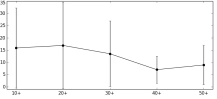
By inspecting the data, we found interesting cor-relations between the number of complex words an-notated and volunteers’ age or English proficiency level. Figures 1 and 2 illustrate average and stan-dard deviation values using 10-year age bands and proficiency levels, respectively.

Figure 1:Age bands over number of complex words

Both graphs show that, although the average num-ber of complex words drops as age and proficiency level increase, the variance within each group is very high, suggesting that such groups may not be signif-icantly distinct from each other. By performing F-tests withp= 0.05, we found a significant difference

between the band of 40+ years of age and the bands

Figure 2:Proficiency levels over number of complex words

of 10+, 20+ and 30+ years of age, which suggests that one’s English knowledge peaks at such age. We also found significant differences between almost all English proficiency levels above A2, except between B2 and C1. We did not find significant differences among education levels.

4.2 Analysis of Data Sources

Evaluating the data, we found that the words deemed complex by Wikipedia editors were marked as com-plex by our annotators in only0.8% of the CW in-stances, and19.7% of the LexMTurk instances. In contrast,51.9% of the edited words in the CW

cor-pus and 40.8% of those in the LexMTurk corpus

were deemed complex by at least one of our anno-tators. As for the remaining Simple Wikipedia in-stances, we found that at least one word in27.3%

of the instances was deemed complex by an anno-tator, which shows that the simplified version of Wikipedia may still be challenging to non-native speakers.

We also inspected these and other datasets for the purposes of LS. In addition to the aforementioned CW and LeXMturk corpora, we took the dataset used in the English Lexical Simplification task of SemEval 2012, composed of 2,010 instances total, and LSeval, the LS evaluation dataset introduced by (De Belder and Moens, 2012), composed by 430 in-stances. Each instance in all these datasets contains a sentence and a target complex word. Table 1 shows the number of target words included in each dataset, how many of them appear in at least one of our 9,200 sentences, and the proportion of the latter that was deemed complex by at least one of our annotators.

Total Appear in 9,200 Complex

CW 272 260 34.6%

LexMTurk 454 420 33.3%

SemEval 410 342 26.0%

LSeval 80 59 20.3%

Table 1:Results of dataset analysis

needs with respect to simplification. 4.3 Features of Complex Words

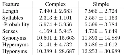
We collected statistics that highlight the differences between simple words and those deemed complex by at least one annotator. We consider words’ log-probability in a trigram language model built from the Simple Wikipedia corpus (Kauchak, 2013), their length, number of syllables, and number of senses, synonyms, hypernyms and hyponyms registered in Wordnet (Fellbaum, 1998). Table 2 shows average values for these features. According to F-tests with

p= 0.01, for all features considered, complex and

simple words are significantly different. On aver-age, complex words are less ambiguous, shorter, and occur less in Simple Wikipedia.

Feature Complex Simple Length 7.490±2.683 7.966±2.724

Syllables 2.313±1.101 2.557±1.163

-Probability 5.974±5.956 5.599±3.784

Senses 4.169±5.945 4.739±5.649

Synonyms 10.501±15.663 11.893±14.889

Hypernyms 3.141±4.732 3.586±4.612

Hyponyms 10.389±28.687 12.253±30.989

Table 2:Mean and standard deviation for word features

We also noticed that the words most frequently deemed complex by annotators were nouns of tech-nical nature, such as “undercroft”, “malleus” and “chalybeatus”.

4.4 Agreement Analysis

We calculated the Krippendorff’s Alpha agreement coefficient (Hayes and Krippendorff, 2007) for each set of 10 sentences that were annotated by 20 volun-teers. The Cohen’s Kappa coefficient (Cohen, 1968) was not used due to the large disparity between the number of complex and simple words, which causes the likelihood of annotators agreeing by chance to be higher than the relative observed agreement. The sets have an average agreement coefficient of0.244,

and a standard deviation of0.1. The relatively low

agreement value highlights the expected heterogene-ity among non-native speakers with different lan-guage backgrounds and proficiency levels.

5 Datasets

We have created two training datasets for the task: joint and decomposed. Both contain all instances which were annotated by 20 non-native speakers. The joint dataset contains a single label for each instance, which is 1 if at least one of the 20 anno-tators has deemed it complex, and 0 otherwise. Dif-ferently, thedecomposeddataset contains one label for each of the 20 annotators, which is 1 if they have judged it to be complex, and 0 otherwise. Along with the labels, the dataset instances also include the sentence, target word and its position. Partic-ipants were allowed to use any additional external resources to build their models. A participant could, for an example, use other (not necessarily publicly available) datasets to complement the one provided. The test set is composed by all the instances annotated by only one non-native speaker. While the training sets contain the data pertaining to the same 2,237 instances, the test set contains 88,221 instances. Using this setup, we are able to replicate a realistic scenario in Text Simplification, where the needs of many readers must be predicted based on the needs of a sample of the reader population.

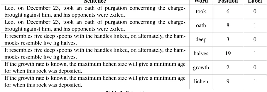
Table 3 shows some examples of instances from ourjointtraining set.

6 Systems

Each team was allowed to submit at most two sys-tems. In total, 42 systems were submitted by 21 teams:

AI-KU Introduces two SVM classifiers trained with a Radial Basis Function over the joint dataset. While one of their systems use as features the word embeddings of the target word itself and its sub-strings (native), the other uses the embeddings of the surrounding words as well (native1).

Sentence Word Position Label Leo, on December 23, took an oath of purgation concerning the charges

brought against him, and his opponents were exiled. took 6 0 Leo, on December 23, took an oath of purgation concerning the charges

brought against him, and his opponents were exiled. oath 8 1 It resembles five deep spoons with the handles linked, or, alternately, the

ham-mocks resemble five fig halves. deep 3 0

It resembles five deep spoons with the handles linked, or, alternately, the

ham-mocks resemble five fig halves. halves 19 1

If the growth rate is known, the maximum lichen size will give a minimum age

for when this rock was deposited. growth 2 0

If the growth rate is known, the maximum lichen size will give a minimum age

for when this rock was deposited. lichen 9 1

Table 3:Dataset instances

Amrita-CEN Introduces two SVM classifiers trained over the joint dataset. While one of them uses word embeddings as well as various semantic and morphological features (w2vecSim), the other also includes POS tag information (w2vecSimPos). BHASHA Presents two systems: an SVM (SVM) classifier and a Decision Tree (DECISIONTREE) classifier. The instances in the dataset are first pre-processed, then classified according to various lexi-cal and morphologilexi-cal features. Finally, the results are post-processed with hand-crafted rules. Both systems are trained over the joint dataset.

ClacEDLK Uses Random Forests to train two classifiers over the joint dataset with semantic, mor-phological, lexical and psycholinguistic features. While one classifier uses a class-assignment thresh-old of 0.5 (RandomForest-0.5), the other uses a threshold of0.6(RandomForest-0.6).

CoastalCPH Introduces a Neural Networks and a Logistic Regression solution. Their Neural Net-works system (NeuralNet) is trained over the joint dataset, and uses two hidden layers leading to a sin-gle activation node. Their Logistic Regression sys-tem (Concatenation) is trained over the decomposed dataset. Both systems use the same set of features, which include word frequency measures and word embedding values.

GARUDA Presents two solutions: a hybrid model (HSVM&DT) and an SVM classifier ensemble (SVMPP). HSVM&DT obtains predictions from various SVM models, which are then validated by Decision Tree classifiers trained specifically to judge

whether the predictions are correct. The validated predictions are then combined into a final label. SVMPP trains a single SVM classifier for each of the 20 annotators of the decomposed dataset, then uses a weighted average to combine their predic-tions.

HMC Performs CWI through a Decision and a Regression Tree, both with a maximum depth of four. During training, their systems deem complex those words which were judged so by at least 25% (DecisionTree25) and 5% (RegressionTree05) of the first 19 annotators in the decomposed dataset. Their systems are then tuned based on the judgment of the 20th annotator.

IIIT Resorts to Nearest Centroid Classification to perform CWI. While one of their classifiers uses the Manhattan distance during training (NCC), the other uses the Euclidean distance (NCC2). As features, they use semantic and morphological features. Their systems are trained over the joint dataset.

JUNLP Presents a Random Forest (RandomFor-est) and a Naive Bayes (NaiveBayes) classifier trained over the joint dataset. Among the semantic, Lexicon-Based and morphological features used are the words’ POS tag and Named Entity information.

MACSAAR Introduces a Random Forest (RFC) and an SVM (NNC) classifier. They use Zipfian features, such as the percentile ranking of the tar-get word, and character n-gram features, such as the probability sum of all character n-grams in the sen-tence. For training, they use the joint dataset.

MAZA Employs ensemble methods over the joint dataset. They train a context-independent system (A) that uses various word frequency features, and a context-aware system (B) that also includes fre-quency of the previous and following words.

Melbourne Uses weighted Random Forest clas-sifiers along with various lexical and semantic fea-tures. While one of their systems attributes weight

1.5 to the complex class (runw15), the other

at-tributes weight 3 (runw3).

PLUJAGH Presents two Threshold-Based solu-tions to CWI. Their first system (SEWDF) judges a word to be complex if its frequency in Simple Wikipedia is lower than 147. Their other system learns the frequency threshold from the joint dataset that maximises the F-Score (SEWDFF).

Pomona Uses Threshold-Based bagged classifiers with bootstrap re-sampling. The thresholds of their classifiers are determined through brute-force over the target words’ frequencies in a given corpus. They use bag sizes of 10 re-samplings selected through 10-fold cross validation, repeated 20 times. The corpora used are Wikipedia (NormalBag) and the Google Web Corpus (GoogleBag). Their sys-tems are trained over the joint dataset.

Sensible Provides a solution that combines Recur-rent Neural Networks and Ensemble Methods. Their Neural Networks are composed of Long Short-Term Memory layers leading to a single activation node. They predict that a word is only complex if the activation node outputs a value equal or big-ger than0.5. The architecture of their networks is

determined through cross-validation over the joint dataset. While one of their systems consist of the best performing Neural Network architecture found (Baseline), the other combines the five best architec-tures using an eXtreme gradient boosted ensemble (Combined).

SV000gg Employs two System Voting techniques that combine various Lexicon-Based, Threshold-Based and Machine Learning voter sub-systems into one. Their first system (Hard) uses Hard Vot-ing: it increases the prediction likelihood of a la-bel by one for each voter that has predicted it for a given instance. Their second system (Soft) uses Performance-Oriented Soft Voting: instead of in-creasing it by one, they increase it by the systems’ G-Score over a held-out portion of the joint dataset. Their voters use a total of 69 morphological, lexical, collocational and semantic features.

TALN Uses Random Forests to perform CWI. While one of their systems is trained over the joint dataset (RandomForest SIM), the other is trained over the decomposed dataset (RandomForest WEI), and includes the number of annotators that deemed the word to be complex as a feature. Both systems also include various lexical, morphological, seman-tic and syntacseman-tic features.

USAAR Presents two Bayesian Ridge classifiers. Their first system (Entropy) is trained based solely on a hand-crafted Word Sense Entropy metric, which is calculated for each target word in the joint dataset. Their other system (Entroplexity) combines Word Sense Entropy with perplexity measures cal-culated with a language model.

UWB Performs CWI with the help of Maxi-mum Entropy classifiers. Both classifiers use only one feature: document frequencies of words in Wikipedia. While one of them is trained over the joint dataset (All), the other is trained over the de-composed dataset (Agg).

7 Baselines

Along with the submitted systems, we include eleven baselines:

• All Complex: Predicts that all words are com-plex.

• All Simple: Predicts that all words are simple.

• (TB) Wikipedia: Threshold-Based approach that exploits the word’s language model proba-bilities from Wikipedia.

• (TB) Length: Threshold-Based approach that exploits the word’s length.

• (TB) Senses: Threshold-Based approach that exploits the word’s number of senses.

• (LB) Ogden: Lexicon-Based approach that classifies as simple words which are in the Og-den’s vocabulary1_.

• (LB) Simple Wiki: Lexicon-Based approach that classifies as simple words which are in the Simple Wikipedia.

• (LB) Wikipedia: Lexicon-Based approach that classifies as simple words which are in Wikipedia.

We train 3-gram language models with SRILM (Stolcke, 2002). The Wikipedia and Simple Wikipedia corpora are the ones made available by (Kauchak, 2013). Sense counts were extracted from WordNet (Fellbaum, 1998).

For completion, we also assess the performance of two ensemble methods:

• (HV) All Systems: Ensemble approach that combines all systems submitted, including the aforementioned baselines, through Hard Vot-ing, in which the final label of each instance is the one that was most frequently predicted by the systems.

• (HV) No Baselines: Identical to the previous baseline, except it does not include our base-lines.

8 Evaluation

To assess the systems’ performance, we choose to complement the typical F-score, which is the har-monic mean between Precision and Recall. Even though F-score is arguably the most frequently used evaluation metric to compare the performance of classifiers, we feel that, as far as the relationship between Complex Word Identification and Lexical

1_{http://ogden.basic-english.org/words.html}

Simplification are concerned, it does not accurately capture the effectiveness of a solution for the task.

To motivate our decision, we must first outline the characteristics of a great lexical simplifier. In order to be both effective and reliable, it must accomplish two things simultaneously:

1. Not to make any replacements that compromise the sentences’ grammaticality and/or meaning.

2. To make a text as simple as possible.

In order to help a simplifier achieve these goals, a complex word identifier must consequently:

1. Avoid labeling complex words as simple, and hence impede them from being simplified.

2. Avoid labeling simple words as complex, and hence allow for unnecessary, possibly erro-neous simplifications.

3. To capture as many complex words as possible, and hence maximise the simplicity of a sen-tence.

Now that we have outlined what the ideal identi-fier must do, we can translate these objectives into typical evaluation expressions used in the context of classification problems. In this context, “positive” and “negative” decisions refer to labeling words as complex and simple, respectively.

While objectives number one and two state that the identifier must minimise the number of false neg-atives and false positives, item three states that it must maximise the number of true positives. One way to measure the proficiency of a classifier in achieving these goals is throughAccuracyand Re-call, respectively. In order to balance these two met-rics, we have conceived the G-score, which mea-sures the harmonic mean between Accuracy and Re-call. For completion, we also report the systems’ ranking according toF-score.

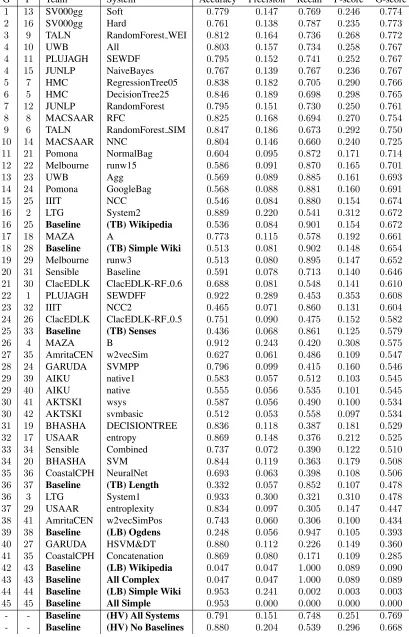
9 Results

G F Team System Accuracy Precision Recall F-score G-score

1 13 SV000gg Soft 0.779 0.147 0.769 0.246 0.774 2 16 SV000gg Hard 0.761 0.138 0.787 0.235 0.773 3 9 TALN RandomForest WEI 0.812 0.164 0.736 0.268 0.772

4 10 UWB All 0.803 0.157 0.734 0.258 0.767

4 11 PLUJAGH SEWDF 0.795 0.152 0.741 0.252 0.767 4 15 JUNLP NaiveBayes 0.767 0.139 0.767 0.236 0.767 5 7 HMC RegressionTree05 0.838 0.182 0.705 0.290 0.766 6 5 HMC DecisionTree25 0.846 0.189 0.698 0.298 0.765 7 12 JUNLP RandomForest 0.795 0.151 0.730 0.250 0.761 8 8 MACSAAR RFC 0.825 0.168 0.694 0.270 0.754 9 6 TALN RandomForest SIM 0.847 0.186 0.673 0.292 0.750 10 14 MACSAAR NNC 0.804 0.146 0.660 0.240 0.725 11 21 Pomona NormalBag 0.604 0.095 0.872 0.171 0.714 12 22 Melbourne runw15 0.586 0.091 0.870 0.165 0.701

13 23 UWB Agg 0.569 0.089 0.885 0.161 0.693

14 24 Pomona GoogleBag 0.568 0.088 0.881 0.160 0.691

15 25 IIIT NCC 0.546 0.084 0.880 0.154 0.674

16 2 LTG System2 0.889 0.220 0.541 0.312 0.672 16 25 Baseline (TB) Wikipedia 0.536 0.084 0.901 0.154 0.672

17 18 MAZA A 0.773 0.115 0.578 0.192 0.661

18 28 Baseline (TB) Simple Wiki 0.513 0.081 0.902 0.148 0.654 19 29 Melbourne runw3 0.513 0.080 0.895 0.147 0.652 20 31 Sensible Baseline 0.591 0.078 0.713 0.140 0.646 21 30 ClacEDLK ClacEDLK-RF 0.6 0.688 0.081 0.548 0.141 0.610 22 1 PLUJAGH SEWDFF 0.922 0.289 0.453 0.353 0.608

23 32 IIIT NCC2 0.465 0.071 0.860 0.131 0.604

24 26 ClacEDLK ClacEDLK-RF 0.5 0.751 0.090 0.475 0.152 0.582 25 33 Baseline (TB) Senses 0.436 0.068 0.861 0.125 0.579

26 4 MAZA B 0.912 0.243 0.420 0.308 0.575

27 35 AmritaCEN w2vecSim 0.627 0.061 0.486 0.109 0.547 28 24 GARUDA SVMPP 0.796 0.099 0.415 0.160 0.546 29 39 AIKU native1 0.583 0.057 0.512 0.103 0.545 29 40 AIKU native 0.555 0.056 0.535 0.101 0.545 30 41 AKTSKI wsys 0.587 0.056 0.490 0.100 0.534 30 42 AKTSKI svmbasic 0.512 0.053 0.558 0.097 0.534 31 19 BHASHA DECISIONTREE 0.836 0.118 0.387 0.181 0.529 32 17 USAAR entropy 0.869 0.148 0.376 0.212 0.525 33 34 Sensible Combined 0.737 0.072 0.390 0.122 0.510 34 20 BHASHA SVM 0.844 0.119 0.363 0.179 0.508 35 36 CoastalCPH NeuralNet 0.693 0.063 0.398 0.108 0.506 36 37 Baseline (TB) Length 0.332 0.057 0.852 0.107 0.478 36 3 LTG System1 0.933 0.300 0.321 0.310 0.478 37 29 USAAR entroplexity 0.834 0.097 0.305 0.147 0.447 38 41 AmritaCEN w2vecSimPos 0.743 0.060 0.306 0.100 0.434 39 38 Baseline (LB) Ogdens 0.248 0.056 0.947 0.105 0.393 40 27 GARUDA HSVM&DT 0.880 0.112 0.226 0.149 0.360 41 35 CoastalCPH Concatenation 0.869 0.080 0.171 0.109 0.285 42 43 Baseline (LB) Wikipedia 0.047 0.047 1.000 0.089 0.090 43 43 Baseline All Complex 0.047 0.047 1.000 0.089 0.089 44 44 Baseline (LB) Simple Wiki 0.953 0.241 0.002 0.003 0.003 45 45 Baseline All Simple 0.953 0.000 0.000 0.000 0.000

- - Baseline (HV) All Systems 0.791 0.151 0.748 0.251 0.769

- - Baseline (HV) No Baselines 0.880 0.204 0.539 0.296 0.668

SV000gg team, which combine various Threshold-Based, Lexicon-Based and Machine Learning ap-proaches with minimalistic voting techniques. Simi-larly, the system from the TALN team, which has the third highest G-score, uses an ensemble method that combines various Decision Tree classifiers. Interest-ingly, the (HV) All Systems and (HV) No Baselines systems, which combine the submitted systems us-ing the same Hard Votus-ing strategy employed by the runner up SV000gg-Hard, did not manage to outper-form it.

One of the most clearly highlighted phenomena in our results is the recurring effectiveness of Deci-sion Trees and Random Forests in CWI: out of the systems with the 10 best G-scores, only three do not employ them. Their reliability is also highlighted by the variety of distinct feature sets used to train them, which range from morphological to syntactic. In contrast, the scores obtained by the BHASHA-DECISIONTREE and GARUDA-HSVM&DT sys-tems reveal that these techniques can be much less effective when incorporated in more elaborate se-tups.

When it comes to F-score, Decision Trees and Random Forests remain dominant among the top 10 systems, but ultimately lose to a much more mini-malistic Threshold-Based strategy. The PLUJAGH-SEWDFF system, which obtained the highest F-score, simply learns the threshold of word frequen-cies in Wikipedia that maximises the F-score over the joint dataset. Similarly, the LTG systems, which achieved the second and third highest F-scores, use Decision Trees to learn a threshold over the number of annotators that judged a word to be complex.

Another interesting finding refers to the difference between raw word frequencies and single-word lan-guage model probabilities. The systems submitted by the PLUJAGH team, which learn thresholds over raw word frequencies from Simple Wikipedia, have consistently outperformed the “(TB) Simple Wiki” baseline, which uses language model probabilities, in both G and F-scores.

Perhaps the biggest surprise from our results comes from to the overall performance of systems which employ Neural Networks and/or word embed-ding models: systems that do so – the ones submit-ted by AI-KU, AmritaCEN, CoastalCPH and Sen-sible – ranked no better than 20th in G-score and

31th in F-score. This comes as a surprise, given that these techniques have been employed in state of the art solutions to a range of tasks in recent years. We hypothesize that the small amount of training data available is the main cause for their unsatisfactory performance.

10 Conclusions

In this paper we have described the findings of the Complex Word Identification task of SemEval 2016. The task was framed as a simple, accessible and yet interesting challenge, such that researchers with any background can participate. It attracted a very large number of participants, particularly given that this was its first edition.

To create the task’s dataset, we conducted a user study with 400 non-native English speakers, which resulted in a total of 158,624 individual annotations. By analyzing the data obtained we were able to con-firm that, according to non-native speakers of En-glish, there is a statistically significant difference be-tween complex and simple words. We have also found a noticeable correlation between the num-ber of complex words annotated and English pro-ficiency level, which is positive evidence that our CWI datasets do, at least to some extent, capture the CWI needs of non-natives. In contrast, we have found that other available resources, such as the CW, LexMTurk and LSeval datasets, may not necessarily do so.

im-portant role.

In the future, we plan to propose more SemEval tasks in the Text Simplification domain, so that we can continue to learn about word complexity, and hopefully further increase this topic’s reach and pop-ularity.

References

John Carroll, Guido Minnen, Darren Pearce, Yvonne Canning, Siobhan Devlin, and John Tait. 1999. Sim-plifying text for language-impaired readers. In Pro-ceedings of the 9th EACL, pages 269–270.

Jacob Cohen. 1968. Weighted kappa: Nominal scale agreement provision for scaled disagreement or partial credit.Psychological bulletin, 70:213.

Jan De Belder and Marie-Francine Moens. 2012. A dataset for the evaluation of lexical simplification. In

Proceedings of the 13th CICLING.

Siobhan Devlin and John Tait. 1998. The use of a psy-cholinguistic database in the simplification of text for aphasic readers. Linguistic Databases, pages 161– 173.

Christiane Fellbaum. 1998. WordNet: An Electronic Lexical Database. Bradford Books.

Andrew F. Hayes and Klaus Krippendorff. 2007. An-swering the call for a standard reliability measure for coding data. Communication Methods and Measures, 1.

Colby Horn, Cathryn Manduca, and David Kauchak. 2014. Learning a lexical simplifier using wikipedia. InProceedings of the 52nd ACL, pages 458–463. David Kauchak. 2013. Improving text simplification

lan-guage modeling using unsimplified text data. In Pro-ceedings of the 51st ACL, pages 1537–1546.

Llus Padr and Evgeny Stanilovsky. 2012. Freeling 3.0: Towards wider multilinguality. InProceedings of the 2012 LREC.

Gustavo H. Paetzold and Lucia Specia. 2013. Text sim-plification as tree transduction. InProceedings of the 9th STIL.

Gustavo H. Paetzold. 2013.Um sistema de simplificac¸˜ao autom´atica de textos escritos em inglˆes por meio de transduc¸ao de ´arvores. State University of Western Paran´a.

Matthew Shardlow. 2013a. A comparison of techniques to automatically identify complex words. In Pro-ceedings of the 51st ACL Student Research Workshop, pages 103–109.

Matthew Shardlow. 2013b. The cw corpus: A new resource for evaluating the identification of complex

words. InProceedings of the 2nd Workshop on Pre-dicting and Improving Text Readability for Target Reader Populations, pages 69–77.

Matthew Shardlow. 2014. Out in the open: Finding and categorising errors in the lexical simplification pipeline. InProceedings of the 9th LREC.