Performance evaluation of a MIMO channel model for simplified OTA test systems

(1)

R E S E A R C H

Open Access

Performance evaluation of a MIMO channel

model for simplified OTA test systems

Sahrul Pasisingi, Katsuhiro Nakada, Akira Kosako and Yoshio Karasawa

*

Abstract

This paper shows performance evaluation results of the proposed multiple-input multiple-output (MIMO) channel model with simplified configuration for OTA measurement systems. The key feature of our proposal is the adoption of a simple antenna branch-controlled configuration for generating various Rayleigh fading environments

composed of a number of multipath delayed waves. The scheme matches well with FPGA implementation with IF band signal processing. The channel model and its theoretical background, and the basic configuration of the measurement system are presented. From an eigenvalue analysis of the generated channel matrix, it is verified that an 8-probe antenna system can realize a very accurate multipath environment for the performance measurement of a 2 × 2 MIMO system, while a 12- or 16-probe antenna system can do the same for a 4 × 4 MIMO system.

Keywords:MIMO; OTA; Fading emulator; Wideband channel; Propagation channel model

1. Introduction

Over-the-air (OTA) test methods are of growing interest for the evaluation of multiple-input multiple-output (MIMO) terminals in LAN, WiMAX, LTE, and other wireless communication systems that adopt MIMO tech-nologies. In OTA testing, a realistic propagation environ-ment is generated around the receiving terminals for measurement of transmission performance characteristics. For OTA system development, the multipath propagation channel models that have been proposed thus far, such as [1-4], have been used in clarifying fundamental con-cepts. Standardization of OTA measurement methods is currently under consideration by the Third Generation Partnership Project (3GPP) [5].

In OTA test methods, the environment for MIMO terminal evaluation is generated by either a reverberation chamber or a fading emulator [5,6]. In the reverberation chamber system, a chamber with metallic walls that effect-ively reflect waves is used to generate a rich multipath propagation environment [5,7]. In fading emulator systems, hereinafter denoted as FE systems, a number of virtual scat-tering probe antennas are positioned circularly around the terminals being tested (devices under test, DUTs) in order to generate a fading environment [8-13]. Although both

methods have advantages and limitations, we investigated FE OTA systems with a focus on channel control flexibility. Among FE MIMO-OTA systems, time-varying multipath signal generation using an available fading simulator scheme is a promising candidate in 3GPP [5] because the fading simulator is able to flexibly control propagation parameters such as delay spread, Doppler spread, and angular spread. Although this type of system can easily realize all necessary functions, the construction cost is generally extremely high. Therefore, in our previous papers [14,15], we proposed an FE MIMO-OTA system with a simplified configuration named as the antenna branch-controlled system and carried out narrowband experiments without any delayed paths. In addition, field-programmable gate array (FPGA) implemen-tation of the proposed scheme has been conducted [16]. Al-though performance identification of the proposed channel model is essential for system development, quantitative evaluations have not yet been achieved in previous papers.

Accordingly, in this paper, after introducing the channel model and its theoretical background, we will make clear the generated channel performance as a function of the number of probe antennas. From an eigenvalue analysis of the generated channel matrix, we verify that an 8-probe antenna system can realize a very accurate multipath environment for the performance measurement of a 2 × 2 MIMO system, while a 12- or 16-probe antenna system can do the same for a 4 × 4 MIMO system.

* Correspondence:[email protected]

The University of Electro-Communications, 1-5-1 Chofugaoka, Chofu, Tokyo 182-8585, Japan

(2)

2. Antenna branch-controlled FE-type MIMO-OTA system and its channel model

2.1 FE-type MIMO-OTA system

Figure 1 shows the basic configuration of an FE-type MIMO-OTA measurement system. The main components of the system are the transmitting antenna input ports (M, in number), the probe antennas which realize the actual multipath environment (L), the receiving antennas (N) of the device (terminal) under test, and theL×Mnetwork for multipath channel generation. TheL×M network, which connects the transmitting antenna ports and the probe antennas, plays an essential role in controlling the signals used to generate the desired propagation channels.

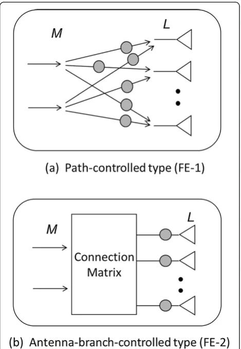
Figure 2 shows two schemes of the FE-type system for generating a multipath fading environment with the time-varying amplitude and phase ofMLpaths. Figure 2a shows the configuration adopted in most available sys-tems. We call this the ‘path-controlled type’ or ‘FE-1’ configuration. As stated above, the FE-1 configuration uses a number of fading simulator units that can flexibly control the amplitude, phase, and delay. Since the use of such high-performance fading simulator units withMLK (K, the number of delayed paths) Rayleigh faders is needed, the cost of system construction is high. Figure 2b, in contrast, is the simplified configuration [14,15] evalu-ated in this paper. We denote this as the‘antenna branch-controlled type’ or ‘FE-2’ configuration. Even when a number of delayed waves are present, the necessary num-ber of Doppler shifters in place of Rayleigh faders isLonly.

In the first stage, the desired spatial correlation charac-teristics between M transmitting antenna ports and Lprobe antennas are realized by a fixed matrix connec-tion. The second stage generates multipath delays and individual Doppler shifts branch by branch. This kind of functional separation results in a very simple and practical configuration. Figure 3 shows a more detailed functional diagram of the proposed system [14]. The FE-2 configuration enables independent Rayleigh fading

for different input signal ports when receiving those signals at a receiving point via a fixed matrix connection using Walsh-Hadamard (WH) codes [14,17]. By suitably adjusting each delayed path weight, the spatial combin-ation of the signals from those antennas produces independent Rayleigh fading. This configuration, unlike FE-1, does not require the generation of any Rayleigh variations in the network. Since it does not include time-varying functions in the signal processing stage, its structure is quite simple and easily constructed.

2.2 Channel model for the FE-2 system

The MIMO channel model for the FE-2 system can be expressed after functional decomposition as follows [14]:

Hðt;τÞ ¼ARXADopplerð Þt Hdelayð Þτ WTX ð1Þ

where matrices WTX, Hdelay, ADoppler, and ARX are the transmission connection matrix, the impulse response

Figure 1General configuration of an FE-type MIMO-OTA system.

Figure 2Functional configuration of‘multipath channel

generation’shown in Figure 1.Gray circle, multipath generation function, namely Rayleigh fader for FE-1 and Doppler shifter for FE-2.

(a)Path-controlled type (FE-1).(b)Antenna branch-controlled type (FE-2).

Pasisingiet al. EURASIP Journal on Wireless Communications and Networking2013,2013:285 Page 2 of 10

(3)

matrix, the Doppler shift matrix, and the reception chan-nel matrix, respectively. All the matrices in the equation are described in detail in [14] and are summarized in Figure 4. Finally, the overall channel impulse response can be obtained by

Hðt;τÞ ¼ XK

k ¼ 1 Að Þk

t

ð Þδ τð − ΔτkÞ ð2aÞ

where

Að Þk

t

ð Þ ¼ að Þnmk ð Þt

n o

ð2bÞ and

að Þnmk ð Þ ¼t

XL

l¼1

wTXlmw k

ð Þ

l ck

ð Þ

ejf2πfDltþ2λπðn−1Þdrcosðθl−θ0Þg:

ð2cÞ

The weight wTX_lm is the element of the TX connec-tion matrix with rowland columnmcomposed of WH codes to realize independent Rayleigh fading for each input portm. The coefficientc(k)is the amplitude of the kth delayed wave, and the weight wl(k)is the coefficient for probe antenna l with delayed path k to realize

Figure 3Detailed functional block diagram of the FE-2 system (proposed configuration).

(4)

independent fluctuations of each delayed path. In the above equation, reception array is adopted as a linear equally spaced array (dr) in the direction of θ0although the channel characteristics, ARX, connecting the probe antenna array to the receiver antenna array as a DUT are more variable than we assumed here. The Doppler shift fDl and direction ofθlfor probe antenna l are dis-cussed below.

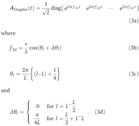
Although the basic formulation has been given in Figure 4 [14], a detailed probe antenna arrangement rule was not given there. Therefore, we give the rule here. The Doppler shift matrix ADoppler is the L×L diagonal matrix for the addition of the Doppler frequency shift to each probe antenna branch signal. In general, ADoppleris automatically determined as a function of the probe an-tenna position in the direction ofθl as well as the oper-ational frequency f and the assumed vehicular speed v. In order to avoid a symmetric arrangement of probe an-tenna positions in the assumed vehicular moving direc-tion, which can cause the same Doppler shift on antenna pairs, we added a small angular offset to each probe an-tenna direction, as shown in Figure 5. The main consid-erations in the determination ofθlare as follows:

1. We must avoid a symmetrical arrangement in the

x-axis direction because the same Doppler shift

frequency appears for the pair of directions. This reduces the variety of Doppler frequencies generated and works as if the number of probe antennas is

smaller than the actual numberL.

2. We must avoid a symmetrical arrangement in the

y-axis direction because the arrangement cancels the

imaginary part of the received signal for the pair of

directions. This causes a deviation from Rayleigh

distribution, as shown in Figure6.

3. We must avoid a symmetrical arrangement about the center point for the same reason stated above.

The above Doppler shift setting problem is important only for the FE-2 system because each probe antenna in the FE-1 system radiates an independent Rayleigh fluctu-ating signal. In order to satisfy the above conditions, we adopted the following arrangement forADoppler:

ADopplerð Þ ¼t

The proposed arrangement is shown in Figure 5. The above Doppler shift setting rule appears to satisfy re-quirements 1 through 3 above. The validity of the assumption is examined in the next section.

Figure 5Doppler shift arrangement for each probe antenna.

0.0001

Figure 6CDF of amplitude distribution for three different

Doppler shift arrangements.

(5)

3. Investigation of the generated channel performance

3.1 Single-input channel characteristics

In this section, we consider the model having channel characteristics of a11(1)(t) with L= 8. We proposed the Doppler shift assignment shown in Figure 5. Figure 6 shows the cumulative distribution functions (CDFs) of the amplitude variations for three different Doppler shift arrangements, i.e., regular positions without any angular offsets, fixed offsets, and double offsets (proposed ar-rangement), with the theoretical Rayleigh distribution. The maximum Doppler shift fDin this simulation is set to be fDTs= 0.01, where Ts is the sampling period. Al-though the regular and fixed offset arrangements have a large discrepancy from the Rayleigh distribution, the proposed arrangement shows very good agreement.

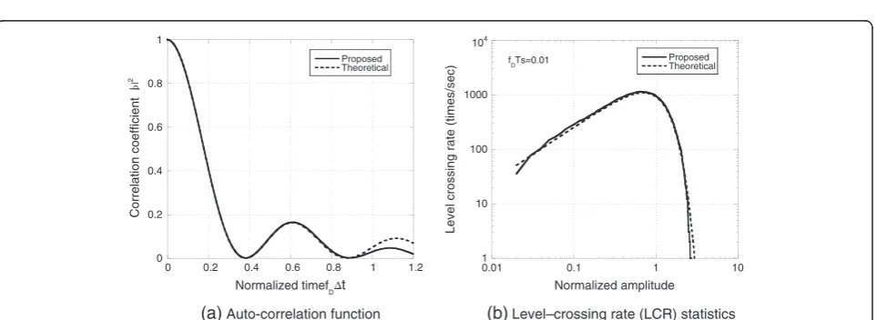
Figure 7 shows the statistics of the time-varying ampli-tude for the proposed Doppler shift arrangement. Figure 7a shows the autocorrelation characteristics, and Figure 7b shows the level crossing rate (LCR) statistics. Based on these figures, there is very good agreement with the theor-etical values. Considering the results for the statistics, we adopt the proposed Doppler shift arrangement shown in Figure 5 for our analysis.

3.2 Eigenvalue characteristics of generated MIMO channels Hereafter, we will give simulation results with parame-ters given in Table 1. The eigenvalues of the MIMO channel are important in evaluating the MIMO trans-mission performance characteristics, such as the bit error rate (BER) and the spectral efficiency in terms of channel capacity. In this section, we discuss the eigen-value statistics of the correlation matrixR(t) defined by

Rð Þ ¼t Að Þ1ð Þt Að Þ1ð Þt

n oH

ð4Þ

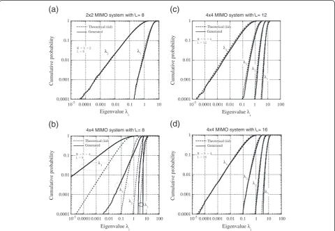
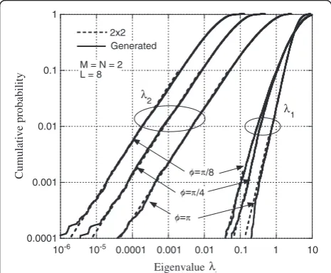
where the superscript H shows the complex conjugate transpose of the matrix. From a practical viewpoint, it seems beneficial for a system to have the smallest pos-sible number of probe antennas L. Since this require-ment is counter to generating an accurate propagation environment, a quantitative evaluation is necessary in order to determine the minimum number of probe an-tennasL. Accordingly, we evaluate the eigenvalue statis-tics of an N × MMIMO system for N=M= 2, 3, and 4 as a parameter ofL. The CDFs of the eigenvalues gener-ated by the simulation and the corresponding independ-ent and idindepend-entically distributed (i.i.d.) Rayleigh cases are compared in Figure 8. As far as the eigenvalue charac-teristics are concerned, L= 8 can realize an ideal envir-onment for the 2 × 2 MIMO system, whileL= 12 or 16 can do the same for the 4 × 4 MIMO system.

For a more quantitative evaluation, we introduce the following measure. In the cumulative probability range of from 0.001 to 0.999, when the maximum difference in decibels between the generated and theoretical eigen-values is within 1 dB, we define this case as‘excellent’, that within 3 dB as‘good’, that within 5 dB as‘fair’, and that beyond 5 dB as ‘poor’, respectively. Table 2 shows this evaluation results for M=N of 2, 3, and 4 with L= 8, 12, and 16. For comparison of the performance, similar simulations of FE-1 have also been carried out, and the obtained results are given in Table 2, which in-dicates that the performance of the FE-1 configuration is slightly superior to that of the FE-2. Even so, a very simple configuration of the antenna branch-controlled configuration (FE-2), which requires only L Doppler shifters instead of the MLK Rayleigh faders needed in the FE-1 system, has a significant advantage from a practical viewpoint.

In order to clarify the dependence of the performance on the number of probe antennas L from a different

0

Level crossing rate (times/sec)

Normalized amplitude f

DTs=0.01

(a) Auto-correlation function (b)Level–crossing rate (LCR) statistics

Correlation coefficient |

(6)

point of view, we carried out the following error analysis icalith eigenvalues corresponding to a cumulative prob-ability of p. The above equation is used to estimate the

normalized absolute deviation of eigenvalues in CDF, where data for cumulative probabilities ranging from 0.001 to 0.999 were taken into consideration. The results are shown in Figure 9, where the 4 × 4 MIMO system with L= 8 has a higher error for both FE-1 and FE-2. For rough estimation, E= 0.2, which corresponds to a normalized eigenvalue of 1 ± 0.2, yields an error of ap-proximately 1 dB so that the error region of E < 0.2 might be sufficiently accurate in practical application. Table 1 Simulation parameters

Parameters Value

Input ports (M) 1 ~ 4

Probe antennas (L) 8, 12, 16

Receive antennas (N) 1 ~ 4

Delay paths (K) 1, 6

Normalized maximum Doppler shift (fDTs) 0.01

Total sampling points 100,000

SNR for channel capacity calculation 10 dB

0.0001

Table 2 Performance comparison of generated environments as viewed from the eigenvalue characteristics

(7)

Thus, the 4 × 4 MIMO system with L= 8 is insufficient from an eigenvalue analysis viewpoint.

Considering that the final performance evaluation measure is the digital transmission characteristic in terms of BER or spectral efficiency, i.e., often referred to as channel capacity, we evaluate the channel capacity performance (in bps/Hz), where equal powers are allo-cated to each input port. Figure 10 shows the results of the channel capacity comparison for a signal-to-noise ratio (SNR) of 10 dB for the FE-2 cases shown in Table 2. In contrast to the large discrepancy of the eigenvalue characteristics shown in Figure 8b, the re-sults forL= 8 for the 4 × 4 MIMO system were in good

agreement. The average channel capacities for the 2 × 2 MIMO system with L= 8 and i.i.d. are 5.63 and 5.55 bps/Hz, respectively, whereas those for the 3 × 3 MIMO system with L= 8, 12, 16, and i.i.d. are 8.47, 8.35, 8.31, and 8.24 bps/Hz, respectively. In addition, the average channel capacities for the 4 × 4 MIMO sys-tem with L= 8, 12, 16, and i.i.d. are 11.23, 11.22, 11.11, and 10.93 bps/Hz, respectively. The channel capacity evaluation indicates that theL= 8 system can serve as a very good performance evaluation tool, even in the case of a 4 × 4 MIMO system.

In the case of eigenmode transmission with multi-stream transmission through each eigenmode path, the overall BER performance may depend on the individual eigenvalue characteristics. In such a case, L= 8 for a 4 × 4 MIMO system is insufficient, as indicated in Figure 8b. However, the results of channel capacity evaluation shown in Figure 10 indicate that the perform-ance depends primarily on the total sum of eigenvalues rather than on the individual eigenvalue characteristics. Figure 11 shows the CDF of the sum of four eigenvalues (λ0=λ1+λ2+λ3+λ4) in the 4 × 4 MIMO system forL= 8, 12, 16, and 32 and the theoretical value under the i.i.d. fad-ing condition. The figure shows that there are no signifi-cant differences even in the case of L= 8. This is the reason why the channel capacity for the 4 × 4 MIMO system with L= 8 shows good agreement with that for L= 12 or 16.

By adopting the WH code matrix forWTX, i.i.d. fluctu-ations for each input port signal can be realized. In some, but not all, cases, an environment having spatial correlation on the transmitting side is required. In the case of M= 2, with an arbitrary value of correlation

0

Average relative error E

The number of probe antennas L

8 12 16 32

Figure 9Normalized average error for anN×NMIMO system.

0 5 10 15

Channel capacity (bit/sec/Hz)

Cumulative probability

Figure 10Channel capacity comparison for anN×N

MIMO system.

Total sum of eigenvalues:

0

Cumulative probability

Type: FE-2

M=N=4

λ

Figure 11CDF of the total sum of eigenvalues of a 4 × 4 MIMO

(8)

coefficient ρTX (real value assumed here) between two input ports, a candidate matrixWTXis as follows:

WTX≡

For a 2 × 2 MIMO system, we carried out a Kronecker model simulation, and the results are shown in Figure 12, which shows that the expected amplitude variations hav-ing a Tx-side spatial correlation are properly generated.

3.3 Wideband characteristics

Specific for wideband system is the fact that several waves with different delays can be resolved in the time domain. In computer simulations, it is easy to handle any number of delayed waves having any delay values. In the present paper, we consider a 2 × 2 MIMO channel withL= 8 having six delayed waves. Figure 13 shows the CDF of each amplitude variation |a11(k)| (k= 1 to 6), where amplitude parameter c(k) is set at 1.0, 0.8, 0.6, 0.4, 0.2, and 0.1 for k= 1, 2,… , 6, respectively. The CDFs of all of the generated delayed path amplitudes follow the

expected CDFs very accurately. The absolute values of the correlation coefficientρ1m(kk′)where

ρðkk0Þ

are given in Table 3. The values in the table, except for those in italics, are approximately 0 or 1 because we can give four orthogonal WH code sets of L= 8 for the weight factor wl(k) in Equation 2c. Accordingly, almost-perfect independent Rayleigh fluctuations are generated

10-6 ₁₀-5 _0.0001 _0.001 _0.01 _0.1 ₁ ₁₀

Figure 12Eigenvalue characteristics of a 2 × 2 MIMO system

withL= 8 considering Tx-side spatial correlation.

0.0001

Figure 13CDF of amplitude variations for each delayed signal.

Table 3 Correlation characteristics among generated delayed waves

að Þ₁₂1 0.0048 0.0029 0.006 0.0053 0.4986 0.0083 að Þ₁₂2 0.0041 0.0062 0.0012 0.0015 0.504 0.4983 að Þ₁₂3 0.0055 0.0009 0.0076 0.0023 0.5047 0.5033 að Þ₁₂4 0.0029 0.0092 0.0023 0.0054 0.4972 0.0108

að Þ₁₂5 0.5023 0.4986 0.498 0.5061 0.0021 0.0071

að Þ₁₂6 0.008 0.5007 0.4958 0.0079 0.0073 0.0039

The values in the table, except for those in italics, are approximately 0 or 1 because we can give four orthogonal WH code sets ofL= 8 for the weight factorwl

(k)

in Equation2c.

(9)

among delayed waves corresponding to k= 1 to 4. For delayed waves corresponding to k= 5 and 6, the correl-ation coefficients are not always 0 because we assigned weighting factors for the delayed waves using random numbers of 1 or −1 due to the lack of an orthogonal code set for L= 8 [14]. When selecting the weighting factors fork= 5 andk= 6, we excluded random code sets having a correlation of more than 0.5. That is the reason why the obtained correlation values are not more than 0.5. All of the delayed waves, including those for k= 5 and 6, can therefore be generated as expected.

4. Conclusions

We evaluated a simplified configuration for OTA test systems. The key element of the proposed model is the adoption of an antenna branch-controlled configuration (FE-2) for generating multipath delayed waves. We in-troduced an orthogonal code weighting for generated delayed waves to realize independent amplitude fluctua-tions among all of the generated delayed paths with mul-tiple input ports, and the performance of the generated channel was evaluated.

Based on the results of the analysis, we reached the following conclusions:

1. By assigning the appropriate Doppler shift to each probe antenna branch, very accurate Rayleigh fluctuations for both amplitude distribution and temporal variation statistics can be generated using eight-probe antennas.

2. From the viewpoint of eigenvalue analysis in generating the MIMO propagation channel, at least 8-probe antennas are necessary for evaluating the 2 × 2 MIMO system, whereas 12- or 16-probe antennas are necessary for the 3 × 3 and 4 × 4 MIMO systems.

3. From the viewpoint of channel capacity analysis, eight-probe antennas are sufficient, even in the case of 4 × 4 MIMO system measurement.

4. By introducing orthogonal code set weighting, almost-independent Rayleigh fluctuations of delayed paths for different input ports are realized with a very simple configuration based on the antenna branch-controlled scheme.

One of the primary practical advantages of the pro-posed scheme is the realization of a flexible MIMO-OTA testing system in a very simplified configuration without the loss of necessary functions or a reduction in performance for the purpose of measurement. Due to the way the fading functions are configured in a cascade, an implementation of the scheme into an FPGA circuit is promising from a practical viewpoint. One disadvan-tage of the proposed scheme is the difficulty involved in

the flexible control of a Tx connection matrix excepting a case of M= 2, as compared to a path-controlled con-figuration (FE-1).

The necessary number of probe antennas in an FE OTA system increases with increasing complexity of the radiation pattern of the DUT or the angular power pro-file of the multipath environment, such as a multicluster environment. Moreover, a dual polarization system re-quires twice the number of probe antennas. For practical applications, typical standard channel models described in Section 6.2 in [5] should be evaluated using the pro-posed model. Since the propro-posed channel model has the capability to realize such standard channel models by setting the parameter values appropriately, we can show calculation examples. However, it seems very difficult to present the evaluation results with a systematic compari-son. Since very careful evaluations are necessary, these evaluations are left for future studies.

Competing interests

The authors declare that they have no competing interests.

Received: 17 August 2013 Accepted: 25 November 2013 Published: 17 December 2013

References

1. JP Kermoal, L Schumacher, KI Pedersen, PE Mogensen, F Frederiksen, A stochastic MIMO radio channel model with experimental validation. IEEE J Sel Areas Commun20(6), 1211–1226 (2002)

2. AF Molish, A generic model for MIMO wireless propagation channels in macro- and microcells. IEEE Trans Signal Proc52(1), 61–71 (2004) 3. MA Jensen, JW Wallace, A review of antennas and propagation for MIMO

wireless communications. IEEE Trans Antennas Propagat52(11), 2810–2824 (2004)

4. W Weichselberger, M Herdin, H Ozcelik, E Bonek, A stochastic MIMO channel model with joint correlation of both link ends. IEEE Trans Wireless Commun5(1), (2006)

5. 3GPP, Measurement of radiated performance for MIMO and multi-antenna reception for HSPA and LTE terminal. Tech Rep (2012). TR37.976 v11.0.0. http://www.quintillion.co.jp/3GPP/Specs/37976-b00.pdf

6. H Arai,Measurement of Mobile Antenna Systems(Artech House, London, 2001)

7. PS Kildal, K Rosengren, Correlation and capacity of MIMO systems and mutual coupling radiation efficiency, and diversity gain of their antennas: simulation and measurements in a reverberation chamber. IEEE Commun Mag42(12), 104–111 (2004)

8. P Kyosti, JP Nuutinen, T Jaemsa, MIMO OTA test concept with experimental and simulated verification, in2010 Proceedings of the Fourth European Conference on Antennas & Propagation, Barcelona, April 2010(IEEE, Piscataway, 2010)

9. H Iwai, K Sakaguchi, T Sakata, A Yamamoto, Proposal of spatial fading emulator dedicated for performance evaluation of handset antennas. IEICE Trans Commun (Japanese Ed.J91-B(9), 960–971 (2008)

10. T Sakata, A Yamamoto, K Ogawa, J Takada, MIMO channel capacity measurement in the presence of spatial clusters using a fading emulator, in

2009 20th IEEE International Symposium on Personal, Indoor and Mobile Radio Communications, Tokyo, September 2009(IEEE, Piscataway, 2009), pp. 97–101 11. C Park, J Takada, K Sakaguchi, T Ohira, Spatial fading emulator for base

station using cavity-excited circular array based on ESPAR, in2004 60th IEEE Vehicular Technology Conference, Los Angeles, September 2004(IEEE, Piscataway, 2004), pp. 256–260

(10)

13. A Scannavini, LJ Foged, MAE Anouar, N Gross, J Estrada, OTA throughput measurements by using spatial fading emulation technique, inFourth European Conference on Antennas and Propagation, Barcelona, April 2010

(IEEE, Piscataway, 2010), pp. 1–5

14. A Kosako, M Shinozawa, Y Karasawa, A simplified configuration of fading emulator system for MIMO-OTA testing. IEICE Trans Commun (Japanese Ed.) J95-B(2), 275–284 (2012)

15. A Kosako, M Shinozawa, Y Karasawa, Simplified configuration of fading emulator system for MIMO-OTA testing, in2011 2nd International Conference on Wireless Communication, Vehicular Technology, Information Theory and Aerospace & Electromagnetic Systems Technology, Chennai, February-March 2011(IEEE, Piscataway, 2011)

16. Y Karasawa, Y Gunawan, S Pasisingi, K Nakada, A Kosako, Development of a MIMO-OTA system with simplified configuration. J Korean Inst Electromagn Eng Sci12(1), 77–84 (2012)

17. P Dent, GE Bottomley, T Croft, Jakes fading model revisited. Electron Lett 29(13), 1162–1163 (1993)

doi:10.1186/1687-1499-2013-285

Cite this article as:Pasisingiet al.:Performance evaluation of a MIMO channel model for simplified OTA test systems.EURASIP Journal on Wireless Communications and Networking20132013:285.

Submit your manuscript to a

journal and beneﬁ t from:

7Convenient online submission

7Rigorous peer review

7Immediate publication on acceptance

7Open access: articles freely available online

7High visibility within the ﬁ eld

7Retaining the copyright to your article

Submit your next manuscript at 7 springeropen.com