A Comparative Analysis of Hierarchical Agglomerative Clustering and Distributed HAC

(1)

CSEIT172411 | Received : 10 July 2017 | Accepted : 13 July 2017 | July-August-2017 [(2)4: 78-85]

78

A Comparative Analysis of Hierarchical Agglomerative

Clustering and Distributed HAC

1

S.Aravindhan,

2

Dr.D.Maruthanayagam

1

Research Scholar, Sri Vijay Vidyalaya College of Arts & Science, Dharmapuri, Tamilnadu, India 2

Head/Professor, PG and Research Department of Computer Science, Sri Vijay Vidyalaya College of Arts & Science, Dharmapuri, Tamilnadu, India

ABSTRACT

In the hierarchical wireless sensor network (WSN), cluster-based network architecture can enhance network self-control capability and resource efficiency, and prolong the whole network lifetime. Thus, clustering has also been a topic of interest in many different disciplines. Finding an energy-effective and efficient way to generate cluster is very important in WSN. This paper describes the well-understood Hierarchical Agglomerative Clustering (HAC) algorithm by provide a Distributed HAC (DHAC) algorithm. With simple six-step clustering, DHAC provides a bottom-up clustering approach by grouping similar nodes together before the cluster head (CH) is selected. DHAC can accommodate both quantitative and qualitative information types in clustering, while offering flexible combinations using four commonly used HAC algorithm methods, SLINK, CLINK, UPGMA, and WPGMA. With automatic CH rotation and re-scheduling, DHAC avoids re-clustering and achieves uniform energy dissipation through the whole network.

Keywords : Wireless Sensor Network, Distributed Hierarchical Agglomerative Clustering (DHAC), Cluster Head,

SLINK, CLINK, UPGMA and WPGMA.

I. INTRODUCTION

Wireless Sensor Network (WSN) is a collection of micro sensor nodes for an intelligent autonomous monitoring system with communication and computing capabilities that are deployed to monitor the areas. It holds the potential to revolutionize many segments of our economy and life, from environmental monitoring. WSN is one of the most important information access platforms, and it is always deployed in extreme environment where people could not survive to obtain information. A WSN is designed to perform a set of high-level information processing tasks such as detection, tracking, or classification. WSNs can be applied in multiple fields such as military, agriculture, traffic, industry, and environmental protection, and it is one of the most important research topics in computer fields [1]. There should be one or a few sink nodes and a number of sensor nodes in WSNs. WSNs should be having a contact with a base station. All sink nodes communicate with base station. Sink node‘s energy is supplied by cable, and it should be unlimited; sensor

node‘s energy is supplied by battery and it is limited. If some sensor nodes‘ energy is exhausted, information from the area monitored by these nodes will not be obtained. And dead nodes will not relay data from other nodes; thus, other sensor nodes will be increasingly burdened with transmission. Given these issues, energy consumption in WSNs is an important research spot. So raising the sensor node‘s energy effi-ciency is an important factor to improve the performance of WSNs. Many researches focus on modifying the sensor node‘s energy efficiency, and designing an efficient routing algorithm is one of the most important approaches [2].

(2)

be deployed, (iii) strong self-organization ability, but these algorithm has a major problem such as (i) flooding mechanism to transmit information (ii) overhead control packets, this kind of routing algorithms are mostly used in small scale of WSNs [4, 5]. The location-based routing algorithm uses location information to guide routing discovery and maintenance as well as data forwarding, enabling directional transmission of the information and avoiding information flooding in the entire network. This algorithm has the advantage as the route would be found very quickly, and the routing information would be accurate, but its efficiency is highly influenced by the geographical environment of WSNs [6].

Chung Horng et al [7] discussed about the HAC Hierarchical Agglomerative Clustering for the wireless sensor network. HAC is a conceptually and mathemati-cally simple clustering approach. HAC has two important categories, divisive and agglomerative. Data types could be either quantitative or qualitative. Resemblance coefficient also has two types, dissimilarity coefficient and similarity coefficient. An input data set for HAC is a component attribute data matrix. Components are the entities that we want to group based on their similarities. Attributes are the properties of the components. Hierarchical routing is the procedure of arranging nodes in a hierarchical manner. It is one of the most popular researches in WSNs, and many typical algorithms are proposed. In this algorithm sensors are divided into several groups based on some characteristics called as cluster. In every cluster, there would be a selected node acts as Cluster Head (CH) which is responsible for collecting data from other nodes in a cluster. All other nodes are called slaves nodes are member nodes. Every cluster head has a connection with the base node or sink node. It will manage every data collected from every cluster head data in WSN. This kind of algorithm has advantages as it is robust and strong and the energy of every node is well balanced. But this algorithm has major limitation such as selection of Cluster head.

Hierarchical agglomerative clustering (HAC) [8] is a conceptually and mathematically simple clustering approach which uses four clustering methods, CLINK, SLINK, UPGMA, and WPGMA. All of these methods comprise three common key steps: obtain the data set, build the similarity matrix, and execute the clustering algorithm. Based on the concept of HAC, DHAC

method was proposed for distributed environments by improving the HAC algorithms. The main idea behind DHAC is that a node only needs one-hop neighbor knowledge to build clusters. To apply the DHAC algorithm in WSNs, a bottom-up clustering approach is followed using simple six steps. Firstly, the qualitative connectivity data is obtained as input data set for DHAC. Secondly, the similarity matrix is built. Thirdly, the similar nodes are grouped together by executing the distributed clustering algorithm. The last three steps are cutting the cluster tree with the threshold, merging the smaller cluster, and electing the CHs. the performance of DHAC is much better than LEACH. The clustering

2.1 Basic Concepts of HAC Algorithm

(3)

uncomplicated and efficient data analysis algorithm, it has been applied to many fields.

2.2 Operation of HAC Algorithm

There are three essential procedures while operating HAC algorithm, which are: obtain input data set, calculate resemblance coefficients and execute HAC algorithm [11]. During the process, various types of data, equations and methods can be applied. The input data can be either quantitative or qualitative, and different types of data need to be processed by different kinds of equation to calculate resemblance coefficients. Further, there are several methods for clustering.

2.2.1. Step 1: obtain the input data set

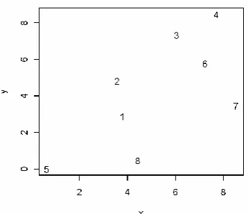
An input data set for HAC is a component–attribute data matrix. Components are the nodes that we want to group based on their similarities. Nodes exchange HELLO messages and obtain neighbor nodes‘ attributes. Attributes are the properties of the components such as the location of nodes, the RSS, the connectivity of nodes, or other features. The type of input data set can be classified into quantitative data and qualitative data. Figure 1, shows a randomly generated 8-node network in the 10x10 m2 field. As illustrated in Table 1a, the location information is used as the quantitative input data. Table 1b uses the one-hop network connectivity data as the qualitative input data, where the ‗‗1‖ value represents a one-hop connection and the ‗‗0‖ value represents no direct connection.

Figure 1: A simple 8-node network.

Table 1: Node input data matrix for the 8-node network.

2.2.2. Step 2: compute the resemblance coefficients

A resemblance coefficient for a given pair of nodes indicates the degree of similarity or dissimilarity between these two nodes. It could be quantitative (e.g., location, RSS) or qualitative (e.g., connectivity). We can calculate Euclidean distance based on the location information by using the Pythagorean Theorem. In Eq. (1), x and y represent the location of node, a and b, on x-axis and y-axis.

Euclidean distance: Dab [(ax - bx) 2 + (ay - by) 2 ] ½

To deal with the qualitative data, there are various ways to calculate the resemblance coefficients [12]. There are three typical methods:

1) Jaccard Coefficient: cxy = a / (a + b + c)

2) Simple Matching Coefficient: cxy = (a + d) / (a + b + c + d)

3) Sorenson Coefficient: cxy = 2a / (2a + b + c)

2.2.3. Step 3: execute the HAC algorithm

(4)

Table 2: Resemblance matrix with quantitative data using Euclidean distance

(2) (3) (4) (5) (6) (7) (8)

(1) 1.94 4.99 6.81 4.27 4.49 4.77 2.51

(2) - 3.54 5.51 5.64 3.79 5.15 4.44

(3) - - 1.99 9.12 1.95 4.59 7.05

(4) - - - 11 2.72 5.07 8.63

(5) - - - - 8.77 8.61 3.83

(6) - - - 2.65 5.99

(7) - - - 5.06

 Single LINKage (SLINK), also called the nearest neighbor method. It defines the similarity measure between two clusters as the minimum resemblance coefficient among all pair entities in the two clusters.

Cslink = Min (C (1,1) ,C(1,2) ,….C(i,j) ,…,C(m,n) )  Complete LINKage (CLINK), also called the

furthest neighbor method. It defines the similarity measure between two clusters as the maximum resemblance coefficient among all pair entities in the two clusters.

Cclink = Max (C (1,1) ,C(1,2) ,….C(i,j) ,…,C(m,n) )  Un-weighted Pair-Group Method using arithmetic

Averages (UPGMA). This defines the similarity measure between two clusters as the arithmetic average of resemblance coefficients among all pair entities in the two clusters. UPGMA is the most commonly adopted clustering method.

CUPGMA = = ∑ (i,j)

 Weighted Pair-Group Method using arithmetic Averages (WPGMA). This is the simple arithmetic average of resemblance coefficients between two clusters without considering the cluster size.

CUPGMA = = ∑ (i,j) Wi

The results of the HAC algorithm are usually depicted by a binary tree or dendrogram, as shown in Fig. 2. The root node of the dendrogram represents the whole data set and each leaf is regarded as a node. The intermediate nodes, thus, describe the extent that the nodes are proximal to each other and the height of the dendrogram. Figure 2 demonstrates three different clustering results for the simple 8-node network depicted in Figure 1 by using SLINK, CLINK, UPGMA methods with quantitative data.

2.2.4. Step 4: cut the hierarchical cluster tree

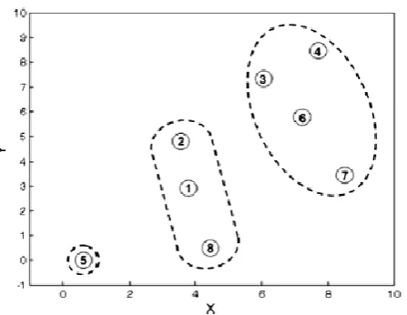
To avoid clusters become oversized and to stop merging of clusters, we make a cut by using a pre-configured threshold value, such as transmission radius, number of clusters, or cluster density. Figure 3b shows a cutting of transmission radius basing on the clustering result of UPGMA with quantitative data. Figure 4 illustrates that the sample network has three corresponding clusters, {3, 6, 4, 7}, {1, 2, 8}, and {5} based on Figure 3b.

Table 3: Resemblance matrix with qualitative data using SORENSON dissimilarity

(2) (3) (4) (5) (6) (7) (8)

(1) 0.5 0.75 1 0.143 0.778 1 0.143

(2) - 0.25 0.429 0.714 0.333 0.667 0.714

(3) - - 0.143 1 0.111 0.667 1

(4) - - - 1 0.25 0.6 1

(5) - - - - 1 1 0

(6) - - - 0.429 1

(7) - - - 1

Step 5: control the minimum cluster size

If the size of a cluster is smaller than the predefined threshold, minimum cluster size, the cluster merges with its closest neighboring cluster. Figure 3 shows that the small Cluster {5} is merged into Clusters {1, 2, 8}. Thus, Figure 5 presents the final formatted clusters {3, 6, 4, 7} and {1, 2, 8, 5}.

2.2.5. Step 6: choose CHs

(5)

Figure 2 : Dendrogram using different the HAC algorithms with quantitative data

In this paper, CHs are the nodes that satisfy two conditions: (i) the node is in the bottom level, which merged into the cluster in the first step and (ii) the node has the lower ID. As demonstrated in Figure 5, nodes 1 and 6 are the CHs of the Cluster {1, 2, 8, 5} and {3, 6, 4, 7}, respectively.

Figure 3: Clustering steps and dendrogram using UPGMA with quantitative data

Figure 4: Generated clusters at Step 4, using UPGMA

with quantitative data

Figure 5: Generated clusters at Step 5, using UPGMA with quantitative data.

III. DISTRIBUTED HIERARCHICAL

AGGLOMERATIVE CLUSTERING (DHAC)

The idea of DHAC is that for WSNs, the HAC algorithm does not actually need the global knowledge. To be specific, a node can make use of only one-hop neighbor knowledge for the computation. Nodes that are far apart will not be grouped into the same cluster anyway. Therefore, it is not necessary to include all the information for clustering. As a result, DHAC can remove the assumption that each node has the global information of every other node. We present the DHAC with the concept of distributed clustering for WSNs based on the quantitative location data and qualitative connectivity knowledge using the different methods. DHAC adopts the ‗‗general assumptions‖ of WSNs as follows:

 The nodes in the network are quasi-stationary.  The nodes are left unattended after deployment.  Each node only has local information or the

identification of its one-hop neighbor nodes.  All nodes have similar capabilities, processing,

communication and initial energy.  Propagation channel is symmetric.

 The transmission ranges of nodes are adjustable. All the nodes have the capability to communicate with the sink directly.

 The sink is static.

3.1. DHAC: cluster formation

(6)

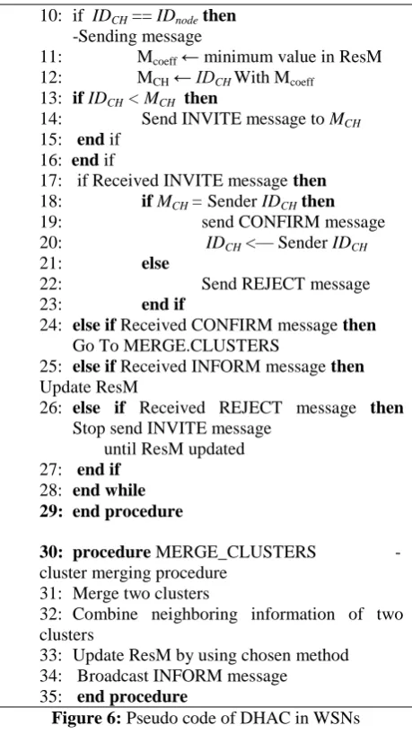
rationale is that every node knows its one-hop neighbors. Figure 6, illustrates the pseudo code of the DHAC implementation for WSNs.

3.1.1. Step 1 and 2: obtain input data set and build resemblance matrix

The procedure ‗‗Set up ResM‖ (Figure 6, lines 1–7) corresponds to ‗‗obtain input data set‖ and ‗‗build resemblance matrix‖ steps are described. To collect input data and set up the local resemblance matrix, in the beginning, each node elects itself as a cluster head and exchanges the information via HELLO messages with its neighbors. In Figure 6, lines 1–7 initialize the clustering process by setting the current IDCH as IDNode and exchanging HELLO messages with one-hop neighbors.

3.1.2. Step 3: execute the DHAC algorithm

After the clustering process ends, each cluster establishes its own local resemblance matrix, from which its minimum coefficient (MCoeff) can be easily found. Each cluster then determines its minimum cluster head (MCH). If the IDNode of the MCH is larger than the CH, the CH will send an INVITE message to the MCH. In Figure 6, lines 10–16 specify two requirements: the sender node must be the current CH, and the sender IDNode must be smaller than MCH. The following illustrates DHAC in detail, step by step:

Definitions:

IDNode : Node ID

IDCH : Cluster Head ID

ResM : Resemblance Matrix Mcoeff : The Minimum_coefficient

in the ResM

MCH : The IDCH of the cluster

corresponds to the Mcoeff in the ResM

CSize : The number of

cluster_member in a cluster

1: procedure SET UP RESM

-exchange information with neighbors 2: IDCH ←IDNode

- self form a singleton cluster

3: Send HELLO message to one-hop neighbors

4: ………

-keep listening from neighbors 5: Receive HELLO messages 6: Establish ResM

24: else if Received CONFIRM message then

Go To MERGE.CLUSTERS

32: Combine neighboring information of two clusters

33: Update ResM by using chosen method 34: Broadcast INFORM message

35: end procedure

Figure 6: Pseudo code of DHAC in WSNs

 In Figure 6, lines 17–23, when a CH receives an INVITE message, it checks the source of the message. If the source is its MCH, the CH sends a CONFIRM message back to the source, selects the source to be the new CH, and turns into the sleep until its resemblance matrix has been updated. For example, Cluster {5} will stop sending the invite message to Cluster {8}.

(7)

and {2}, for instance, will merge their resemblance matrices and their neighbor lists.

 The CH of the new cluster broadcasts an INFORM message to notify its neighbors to update their resemblance matrices (Figure 6, lines 25 and 37). Clusters update their own resemblance matrix after receiving this INFORM message, which contains the new cluster information and the merged neighbor list.

The process will repeat until the while condition (line 9) fails. During the clustering process, all CHs of clusters keep listening. When a CH receives a message, it reacts based on the message type.

3.1.3. Step 4: cut the hierarchical cluster tree

Using a predefined threshold, the while loops in Figure 6, lines 9–28, controls the upper bound size of clusters. The control conditions correspond to the step of cutting the hierarchical cluster tree.

3.1.4. Step 5: control the minimum cluster size

After clusters are generated by running DHAC, the minimum cluster size can also be used to limit the lower bound of cluster size by performing the procedure ‗‗MERGE CLUSTERS‖ (Figure 6, lines 29– 31).

Clustering has been a topic of interest in many different disciplines for a long time. To adapt to the constraints of WSNs, clustering has generated a lot of discussion. This paper advocated the application of well-known the HAC algorithm methods to WSNs and another distributed approach, DHAC algorithm, to classify sensor nodes into appropriate groups instead of simply gathering nodes by their distance to some randomly selected CHs. In this paper demonstrated the well-understood HAC algorithm methods, SLINK, CLINK, UPGMA and WPGMA. Based on the study of the HAC algorithm methods, we illustrated how to use the DHAC approach to mitigate the problems encountered

with current protocols, and we supported the analysis by simulation.

V. REFERENCES

[1]. Stallings W. Wireless communications and networks. 2nd ed. Upper Saddle River, NJ, USA: Prentice Hall; 2005.

[2]. Liu B. Unsupervised Learning. Web Data mining exploring hyperlinks, contents and usage data. 2nd ed. Springer; 2010. p. 134–55.

[3]. Anderberg MR. Cluster Analysis for Applications. New York: Academic Press; 1973.

[4]. Heinzelman WR, Kulic J, Balakrishnan H. Adaptive protocols information in wireless sensor networks. Proceedings of the 5th ACM/IEEE MOBICOM; 1999. [5]. Lung CH, Zhou CJ. Using hierarchical agglomerative

clustering in wireless sensor networks: an energy-efficient and flexible approach. Ad Hoc Networks. 2010; 8(3):328–44.

[6]. Ho JH, Shih HC, Liao BY, Chu SC. A ladder diffusion algorithm using ant colony optimization for wireless sensor networks. Information Sciences. 2012; 192(1):204–12.

[7]. Lung C-H, Zhou C, Yang Y. Applying hierarchical agglomerative clustering to wireless sensor networks. Ad Hoc Networks. 2004; 8(3):328–44.

[8]. Chung-Horng Lung, Chenjuan Zhou, ―Using hierarchical agglomerative clustering in wireless sensor networks: An energy-efficient and flexible approach‖ IEEE "GLOBECOM" 2008 proceedings. [9]. B. S. Everitt, S. Landau, M. Leese, and D. D. Stahl,

Cluster analysis, 5 ed.: WILEY, 2010.

[10]. X. Rui and D. Wunsch, II, "Survey of clustering algorithms," IEEE Transactions on Neural Networks,

vol. 16, pp. 645-678, 2005.

[11]. C. Zhou, "Application and Evaluation o f Hierarchical Agglomerative Clustering in Wireless Sensor Networks," MASc Thesis, Department of Systems and Computer Engineering, Carleton University, Ottawa, Canada, 2008.

[12]. S. S. Choi, S. H. Cha, and C. Tappert, "A Survey of Binary Similarity and Distance Measures," Journal on Systemics, Cybernetics and Informatics, vol. 8, pp. 43-48, 2010.

[13]. M.R. Anderberg, Cluster Analysis for Applications, Academic Press, New York, 1973.

[14].Pal N.R, Pal K, Keller J.M. and Bezdek J.C, ―A Possibilistic Clustering Algorithm‖, IEEE Transactions on Fuzzy Systems, Vol. 13, No. 4, Pp. 517–530, 2005.

(8)

[16].J. C. Dunn (1973): "A Agglomerative Relative of the ISODATA Process and Its Use in Detecting Compact Well-Separated Clusters", Journal of Cybernetics 3: 32-57

[17].

VI. AUTHORS PROFILE

S.Aravindhan received his M.Phil

degree from Thiruvalluvar university,Vellore in the year 2012.He has received his MCA degree from Anna University,Chennai in the year 2011.He is pursuing his Ph.D degree at Sri Vijay Vidyalaya College of Arts & Science (Affiliated Periyar University),Dharmapuri, Tamilnadu, India. His areas of interest include Data Mining, Cloud Computing and Computer Networks.

Dr.D.Maruthanayagam received his