Simulation Optimization Using Soft Computing

Abstract

MEDAGLIA, ANDR´ES L. Simulation Optimization Using Soft Computing. (Under the direction of Dr. Shu-Cherng Fang and Dr. Henry L. W. Nuttle.)

To date, most of the research in simulation optimization has been focused on single response optimization on the continuous space of input parameters. However, the optimization of more complex systems does not fit this framework. Decision makers often face the problem of optimizing multiple performance measures of systems with both continuous and discrete input parameters. Previously acquired knowledge of the system by experts is seldom incorporated into the simulation optimization engine. Furthermore, when the goals of the system design are stated in natural language or vague terms, current techniques are unable to deal with this situation. For these reasons, we define and study thefuzzy single response simulation optimization (FSO) and fuzzy multiple response simulation optimization (FMSO) problems.

The primary objective of this research is to develop an efficient and robust method for simulation optimization of complex systems with multiple vague goals. This method uses a fuzzy controller to incorporate existing knowledge to generate high quality approximate Pareto optimal solutions in a minimum number of simulation runs.

For comparison purposes, we also propose an evolutionary method for solving the FMSO problem. Extensive computational experiments on the design of a flow line manufacturing system (in terms of tandem queues with blocking) have been con-ducted. Both methods are able to generate high quality solutions in terms of Zitzler and Thiele’s “dominated space” metric. Both methods are also able to generate an even sample of the Pareto front. However, the fuzzy controlled method is remarkably more efficient, requiring far fewer simulation runs than the evolutionary method to achieve the same solution quality.

A Olga Luc´ıa, por confiar en mi y su apoyo incondicional.

Biography

Acknowledgments

I thank Dr. Shu-Cherng Fang, for his guidance, responsiveness, and support as an ad-visor. He always went beyond his duties and responsibilities as an advisor and taught me valuable lessons that I will take with me for the rest of my life. Especially, I thank him for his constant encouragement to look deeper into the essence of matters. His dedication to doing the job well is really admirable. I thank Dr. Henry L. W. Nuttle for his support and valuable contributions as co-advisor. Especially, I thank him for his pragmatic view, which on many occasions shed light on my research. He also had the patience and incredible ability to make sense out of my not–always–readable manuscripts. I really appreciate all the time, energy, and resources he invested in me. I thank Dr. Stephen D. Roberts for teaching me the principles of object–oriented simulation, and above all, some principles of life. I thank Dr. James R. Wilson for his thoroughness and for always being encouraging and supportive. His sense of serving the community and passion for teaching are truly inspiring and will guide me through the rest of my life.

I thank the students at the Fuzzy and Neural Group at North Carolina State University. I always found their support on many facets of my life as a graduate student. Special thanks to my “big brothers” Nanchieh Chiu and Ta-Wei Hung for making my life easier. I thank Shyh-Huei Chen, who has been a good friend since the first day I joined the group.

I thank Dr. Marc-david Cohen for his incredible support throughout the time that I have been working at SAS. I especially appreciate his seasoned view of the Operations Research world and I thank him for sharing it with me. I am grateful to my colleagues at SAS, who provided me the perfect escape from school work and helped me relieve the pressure.

thank the Universidad de los Andes and the Fulbright Commission for their initial trust and support.

I have met people that have supported me along my life and they well deserve my gratitude. I thank Carlos L´opez-Duarte, the outstanding instructor who opened my eyes to the exciting world of Operations Research. I thank Carmen Lucila Osorno, who encouraged me to quit my job and pursue a Ph.D., when it seemed like a crazy idea. I thank Luis Pinz´on, Mar´ıa Elsa Correal, Dr. Fernando Palacios, Mario Castillo, and Gonzalo Torres, at the Universidad de los Andes, for their continuing support. They all are among the most encouraging individuals I have ever met. I also thank my very good old friends, Gabriel E. Pardo, Edgar E. Blanco, Juan Diego Londo˜no, and Alejandro Sierra. All of them have provided me the inspiration that true friendship always provides. I also thank my in-laws, Olguita and Rafael Sarmiento, for their continuos support; and my brother-in-law, Ricardo Parra, who has helped me out since the first time I met him. Last, but not least, I thank Ligia Restrepo, my godmother, who has always been there to support me and my family through very rough times. Without her support, I would not have made it through college.

I thank my mother, who has supported me unceasingly since the day she brought me to this world. She has worked extremely hard and sacrificed herself to give me the best education. ¡Gracias mam´a! I thank my father, who despite his short life, taught me many of the most important things in life. I just wish he could be here with me. I thank Alexandra, my sister, who was my very first teacher and always knew how to keep me grounded to reality.

Contents

List of Tables ix

List of Figures x

1 Introduction 1

1.1 Simulation Optimization . . . 1

1.2 Simulation Optimization with Vague Goals . . . 3

1.3 Scope and Objectives of Research . . . 4

1.4 Organization of the Dissertation . . . 5

2 Literature Review 6 2.1 Simulation Optimization . . . 6

2.1.1 Optimization Over a Finite Set . . . 7

2.1.1.1 Multiple Comparison Procedures . . . 7

2.1.1.2 Ranking and Selection . . . 7

2.1.2 Response Surface Methodology . . . 7

2.1.3 Gradient Based Algorithms . . . 8

2.1.3.1 Stochastic Approximation . . . 8

2.1.3.2 Gradient Estimation Techniques . . . 9

2.1.3.2.1 Finite Differences . . . 9

2.1.3.2.2 Perturbation Analysis . . . 10

2.1.3.2.3 Likelihood Ratio Method . . . 10

2.1.3.2.4 Frequency Domain Experimentation . . . . 10

2.1.4 Derivative–free Methods . . . 11

2.1.4.1 Nelder–Mead Based Methods . . . 11

2.1.4.2 Simulated Annealing . . . 11

2.1.5 Other Methods . . . 12

2.1.6 Multicriteria Simulation Optimization . . . 12

2.2 Soft Computing . . . 12

2.2.1 Fuzzy Logic . . . 13

2.2.2 Neurocomputing . . . 13

2.2.3 Evolutionary Computing . . . 14

2.2.3.1.1 Aggregation Approaches 15

2.2.3.1.2 Non Pareto–based Approaches 16

2.2.3.1.3 Pareto–based Approaches 17

2.3 Simulation Optimization and Soft Computing . . . 19

3 A Fuzzy Controlled Approach 20 3.1 Introduction . . . 20

3.2 Proposed Approach . . . 21

3.2.1 Simulator . . . 22

3.2.2 Fuzzy Controller . . . 23

3.2.3 Handling Multiple Criteria . . . 26

3.2.4 Algorithms . . . 28

3.2.4.1 Target Threshold for the FSO Problem . . . 28

3.2.4.2 Pareto Optimization for the FMSO Problem . . . 30

3.3 Knowledge Acquisition . . . 31

3.4 Application to Flow Line Design . . . 35

3.4.1 Introduction . . . 35

3.4.2 Framework . . . 36

3.4.3 Simulator . . . 37

3.4.4 Knowledge Base Design . . . 38

3.4.4.1 State and Control Variables . . . 38

3.4.4.2 Linguistic Data Base Design . . . 39

3.4.4.3 Rule Base Design . . . 40

3.4.4.3.1 Single Antecedent Rules . . . 40

3.4.4.3.2 Multiple Antecedent Rules . . . 41

3.4.5 Computational Experiments . . . 43

3.4.5.1 Single Objective . . . 43

3.4.5.2 Multiple Objectives: Generating the Efficient Frontier 46 3.5 Concluding Remarks . . . 47

4 A Multicriteria Evolutionary Approach 49 4.1 Evolutionary Algorithm . . . 49

4.1.1 Representation . . . 51

4.1.2 Evaluation . . . 52

4.1.3 Fuzzification . . . 52

4.1.4 Fitness Assignment . . . 53

4.1.4.1 Example . . . 57

4.1.5 Selection . . . 59

4.1.7 Approximate Pareto Optimal Set . . . 61

4.1.8 Elitism . . . 61

4.2 Application to the Flow Line Design Problem and Comparison with the Fuzzy Controlled Approach . . . 63

4.3 Conclusions . . . 65

5 An Efficient and Flexible Mechanism for Constructing Membership Functions 68 5.1 Introduction . . . 68

5.2 Membership Function Generation . . . 70

5.2.1 Overview . . . 70

5.2.2 Current Methods . . . 71

5.3 Proposed Mechanism . . . 72

5.3.1 B´ezier Curves . . . 72

5.3.2 Mathematical Framework . . . 73

5.3.3 Methodology . . . 77

5.3.3.1 Basic Operations . . . 77

5.3.3.2 Data–driven Estimation . . . 77

5.4 Performance . . . 82

5.4.1 Flexibility . . . 82

5.4.2 Numerical Examples . . . 83

5.4.3 Computational Efficiency . . . 88

5.5 Conclusion . . . 88

6 Summary and Recommendations 90 6.1 Summary . . . 90

6.2 Recommendations for Future Research . . . 92

A Membership Functions 110 A.1 State Variables . . . 110

A.2 Control Variables . . . 116

B Rule Base for the Multiple Objective Scenario 121

C Results for the Fuzzy Controlled Approach 124

List of Tables

3.1 Flow line simulation inputs ranges . . . 38

3.2 Initial conditions for the single–goal scenario with improved controlla-bility . . . 45

4.1 Evaluated and fuzzified performance measures for E(t). . . 58

4.2 Comparison of fitness assignment methods. . . 59

4.3 Bounds on weights for OSEA experiments. . . 64

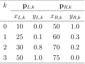
5.1 Control points (before change). . . 83

5.2 Sum of square errors (SSE) . . . 86

5.3 SSE progress for the test benchmark cases (² = 0.0010; †: final solu-tion). . . 86

A.1 Flow line fuzzy controller inputs. . . 111

List of Figures

1.1 Simulation optimization framework . . . 2

3.1 Fuzzy controlled simulation optimization . . . 22

3.2 Target Threshold Algorithm . . . 29

3.3 Pareto Optimization Algorithm . . . 32

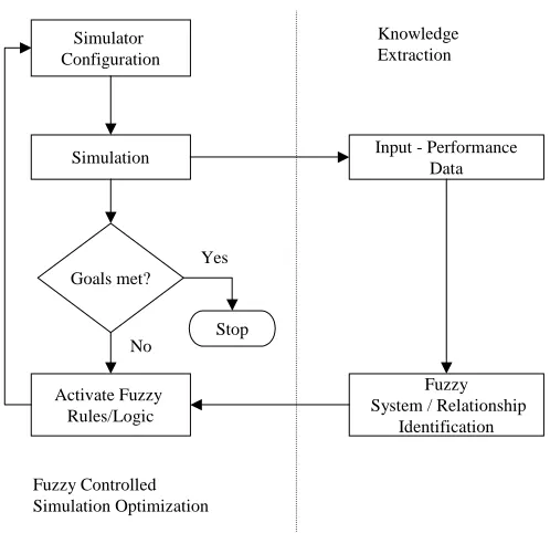
3.4 Fuzzy controlled simulation optimization and knowledge extraction . 34 3.5 Tandem of queues with blocking (flow line) . . . 36

3.6 Flow line optimization framework . . . 37

3.7 Overall work–in–process ($) . . . 39

3.8 Utilization at station 1 (ϕ₁) . . . 39

3.9 Change in server rate at station 1 (∆γ₁) . . . 40

3.10 Correlation coefficients extracted from the full correlation matrix . . . 41

3.11 Response surface for the work–in–process (s₃ = 4, s₄ = 6, b₂ = 4, b₄ = 5, and s₂ = 7) . . . 42

3.12 Response surface for the utilization at station 1 (s₃ = 4,s₄ = 6,b₂ = 4, b₄ = 5, and s₂ = 7) . . . 43

3.13 Control path for the overall work–in–process membership function for the single–goal scenario. . . 45

3.14 Solution for different initial conditions for the single–goal scenario with improved controllability . . . 46

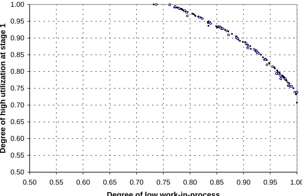
3.15 Approximate Pareto front for the two-goal scenario . . . 47

3.16 Zitzler and Thiele’s dominated space metric [150] for the two-goal sce-nario . . . 48

4.1 Optimal Scoring Evolutionary Algorithm (OSEA) . . . 50

4.2 Representation in OSEA. . . 52

4.3 Optimal fitness in performance space. The symbols N, •, and ¥ rep-resent the first, second, and third tier of optimal scores, respectively. . 60

4.4 Stochastic Universal Sampling . . . 60

4.5 One–point crossover in OSEA. . . 61

4.6 Updating P_approximate∗ (t) . . . 62

4.7 Comparison of the dominated space. . . 65

4.9 Comparison of the Pareto front. . . 66

5.1 Types of membership functions. . . 76

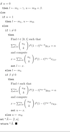
5.2 Finding µ_A˜(x) given x . . . 78

5.3 Finding αA˜ given α . . . 79

5.4 Data–driven estimation of the right membership function . . . 82

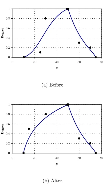
5.5 Effect on the change of a single control point. . . 84

5.6 Data–driven estimation. Data: subject 35 (Old man). . . 85

5.7 Data-driven estimation (²= 0.0010). . . 87

A.1 Overall work-in-process (w) . . . 112

A.2 Work-in-process at stage 1 (w₁) . . . 112

A.3 Work-in-process at stage 2 (w₂) . . . 112

A.4 Work-in-process at stage 3 (w₃) . . . 113

A.5 Work-in-process at stage 4 (w₄) . . . 113

A.6 Time in system (T) . . . 113

A.7 Utilization at station 1 (ρ₁) . . . 114

A.8 Utilization at station 2 (ρ₂) . . . 114

A.9 Utilization at station 3 (ρ₃) . . . 114

A.10 Utilization at station 4 (ρ₄) . . . 115

A.11 Change in server rate at station 1 (∆µ₁) . . . 118

A.12 Change in server rate at station 3 (∆µ₃) . . . 118

A.13 Change in servers at station 2 (∆s₂) . . . 118

A.14 Change in servers at station 3 (∆s₃) . . . 119

A.15 Change in servers at station 4 (∆s₄) . . . 119

A.16 Change in buffer space at station 2 (∆b₂) . . . 119

A.17 Change in buffer space at station 4 (∆b₄) . . . 120

C.1 Experiment # 1 of the two-goal scenario with the fuzzy controlled approach. . . 124

C.2 Experiment # 2 of the two-goal scenario with the fuzzy controlled approach. . . 125

C.3 Experiment # 3 of the two-goal scenario with the fuzzy controlled approach. . . 125

C.4 Experiment # 4 of the two-goal scenario with the fuzzy controlled approach. . . 126

C.5 Experiment # 5 of the two-goal scenario with the fuzzy controlled approach. . . 126

D.1 Experiment # 1 of the flow line design problem with two goals solved by OSEA. . . 127

D.3 Experiment # 3 of the flow line design problem with two goals solved by OSEA. . . 128 D.4 Experiment # 4 of the flow line design problem with two goals solved

by OSEA. . . 129 D.5 Experiment # 5 of the flow line design problem with two goals solved

by OSEA. . . 129 D.6 Experiment # 6 of the flow line design problem with two goals solved

Chapter 1

Introduction

1.1

Simulation Optimization

A system is a collection of entities that act and interact toward the accomplishment of a logical end [116]. In order to study a system rigorously, the system is modeled in the form of logical and mathematical relationships. If the model is simple enough, the performance of the underlying system can be evaluated analytically. Nevertheless, in real–world scenarios, the presence of stochastic elements and complex interactions between the system entities often preclude the possibility of obtaining an analytical solution. In these cases, the model can be studied using simulation. In this disserta-tion, simulation refers to discrete event simulation.

In discrete event simulation, the state of the system may change with the occur-rence of instantaneous events at separate and countable points in time [81]. Real world computer, communication, and manufacturing networks are examples of highly complex systems that are commonly evaluated using discrete event simulation [56, 81, 110, 113].

The simulation approach to problem solving, typically involves a series of trials in which changes are made to the input variables so that resulting changes in the output variables (responses or system performances) can be observed and identified [19]. Even though simulation can provide a very detailed and accurate model, it is in itself more of a descriptive than a prescriptive modeling tool [124].

1.1 depicts a simulation optimization framework. In this framework the output of a complex model is introduced into an optimization strategy which adjusts and feeds the inputs back to the model.

Optimization Strategy Feedback

Inputs _Outputs

Simulation

Figure 1.1: Simulation optimization framework

Formally, the single response simulation optimization (SRSO) problem can be stated as:

min

x∈X f(x) (1.1)

where,f(x) =E[L(x, ω)] is the expected value of the system performance measure of interest, L(x, ω) is the sample performance,ω represents the stochastic effects of the system,xis a vector ofN controllable parameters, andX is a closed set of constraints onx.

The SRSO problem has received much attention by the simulation community. Several reviews on the field of simulation optimization deal almost exclusively with this problem [3, 5, 19, 45, 70, 90, 111]. Brief descriptions of various methods of simula-tion optimizasimula-tion are given in Chapter 2.

In practice, most of the time an analyst has to consider several criteria simulta-neously. In the presence of conflicting objectives, a simulation optimization method must take into account the tradeoff between these criteria. The multiple response simulation optimization (MRSO) problem is:

min

x∈X{(f1(x), f2(x), . . . , fK(x))} (1.2)

Despite of its real world applicability, relatively little research has been conducted on the MRSO problem. Montgomery and Bettencourt [92] use the Geoffrion, Dyer, Feinberg method (GDF) to optimize a simulation model with four criteria and two input parameters. Clayton et al. [25] and Rees et al. [106] use a goal programming approach. Biles and Swain [11, 12] propose and compare a first and second order response surface approach with a direct search algorithm. Evans et al. [36] suggest a set of guidelines for the multicriteria optimization of simulation models. A brief description of these methods is given in Chapter 2.

1.2

Simulation Optimization with Vague Goals

Most of the time the goals for a system are stated in vague natural language by the decision maker. For instance, in a manufacturing setting a decision maker may want to design a system with low work–in–process and high utilization of a certain expensive machine. In this case the vague terms low and high introduced by the decision maker have to be incorporated into the analysis, deduced, and interpreted according to the context. In this setting, the problem is to find the value of the controllable parameters such that all the objectives of the system are satisfied to a high degree.

Fuzzy technology provides a proven and efficient way to compute with words and incorporate natural language into the area of simulation optimization. Fuzzy set theory was first introduced in the 1960s by Lotfi A. Zadeh as a way to capture uncertainty and vagueness often overlooked in the analysis of complex systems [144]. A fuzzy set ˜A is characterized by its membership function µ_A˜, which maps each element of the universe X to the interval [0,1]. This function indicates the degree to which each element belongs to the set.

Rewriting SRSO to incorporate vagueness, we have the fuzzy single response sim-ulation optimization or fuzzy simulation optimization (FSO) problem:

max

x∈X µG˜(f(x)) (1.3)

where, µ_G˜(f(x)) is a measure of the degree of satisfaction of the vague target repre-sented by the fuzzy set ˜Gand, as above,f(x) is the expected value of the performance measure associated with the target,xis the vector ofN controllable parameters, and

MRSO has its corresponding problem that incorporates vagueness, namely the fuzzy multiple response simulation optimization orfuzzy multicriteria simulation op-timization (FMSO) problem:

max

x∈X

©¡

µ_G˜1(f₁(x)), µ_G˜2(f₂(x)), . . . , µ_G˜

K(fK(x))

¢ª

(1.4)

where for k = 1, . . . , K, µ_G˜

k(fk(x)) is the degree of satisfaction of the k-th vague

target represented by the fuzzy set ˜G_k;f_k(x) is the expected value of the performance measure associated with the k-th target.

1.3

Scope and Objectives of Research

The primary objective of this research is to develop an efficient and robust method for the multicriteria optimization of simulated complex systems with vague goals. This method, which uses a fuzzy controller, incorporates existing knowledge, satisfies vaguely stated goals, generates a high quality approximate Pareto optimal set, and is efficient in terms of simulation runs.

To date, most of the research in simulation optimization has been focused on sin-gle response optimization on the continuous space of input parameters X. However, the optimization of more complex systems does not fit this framework. For instance, decision makers often face the problem of optimizing multiple performance measures of systems with both continuous and discrete input parameters. Additionally, pre-viously acquired knowledge of the system by experts has been largely ignored by simulation optimization techniques proposed in the literature. These techniques do not provide any means of incorporating this valuable knowledge into the optimization engine. Furthermore, if the goals of the system design are stated in natural language or vague terms, current techniques are simply unable to deal with this imprecision. Our approach for simulation optimization will take into account the issues of con-tinuous and discrete input parameters, multiple criteria, preexistent knowledge, and vagueness in the system goals.

The objectives of this research may be summarized as follows.

1. Develop methods to solve problems FSO in (1.3) and FMSO in (1.4).

pre-viously acquired knowledge on the system, vagueness in the system goals, and considering multiple criteria.

3. Develop an alternative and competitive approach to unveil the strengths and weaknesses of the proposed approach in 2.

4. Conduct an extensive experimental performance evaluation of the proposed ap-proaches on a Flow Line Design problem.

To validate the mechanisms proposed to achieve objectives 2 and 3, we use the popular trapezoidal fuzzy sets. To further improve the expressive power of the vague concepts used therein, we also

5. Investigate, formulate, and develop an efficient and flexible mechanism to rep-resent virtually any vague concept expressed in natural language.

1.4

Organization of the Dissertation

Chapter 2

Literature Review

In the first part of this chapter, we summarize the existing alternatives to simula-tion optimizasimula-tion. The second part, deals with an overview of soft computing with emphasis on the existing literature on evolutionary multicriteria optimization.

2.1

Simulation Optimization

The dramatic improvement in computer technology, its relatively low cost, and broad availability, have led researchers in industry and academia to increased efforts in the area of simulation optimization of complex systems. Even though a lot of research has been conducted in the last twenty–five years, many problems remain open and unsolved. Due to these loose ends and the high impact on industry, the area keeps growing and attracting researchers and practitioners year after year.

Several reviews on the field of simulation optimization are available [3–5, 19, 39, 45, 52, 70, 90, 111, 119]. The one written by Fu [45] presents an excellent overview of the field. The main forum for simulation researchers and practitioners is the Winter Simulation Conference (WSC). Its proceedings are a valuable source to keep up to date on progress in the area.

2.1.1

Optimization Over a Finite Set

The methods discussed here are useful when the number of choices is not too large, say 2 to 20 [55]. They are basically statistical procedures that fall in one of two categories: multiple comparison or ranking–and–selection.

2.1.1.1 Multiple Comparison Procedures

The purpose of these procedures is the construction of confidence intervals based on pairwise comparisons. Some of the methods in this category are the all–pairwise comparisons based on paired–t confidence intervals and the Bonferroni inequality; multiple comparisons with the best (MCB); and all–pairwise multiple comparisons (MCA) approach. The typical assumptions for these methods are independence and normality of the performance measure of interest. For further details on this subject the reader is referred to Goldsman and Nelson [55] and Law and Kelton [81].

2.1.1.2 Ranking and Selection

Ranking and selection methods are statistical procedures designed to select the best system or a subset of systems that include the best one, from a finite set of choices. Provided some assumptions are met, these methods guarantee that the correct se-lection is made with at least a (user specified) probability. These methods can be classified in two major categories: indifference zone and subset selection. The method proposed by Dudewicz and Dalal [34] falls into the first category, while that proposed by Sullivan and Wilson [123] falls into the subset selection methods category. Both procedures are particularly useful for simulation optimization because they do not re-quire variances to be equal or to be known. Again, for further details on this subject the reader is referred to Goldsman and Nelson [55] and Law and Kelton [81].

2.1.2

Response Surface Methodology

of input parameters. Once a regression model is estimated, it is treated as a deter-ministic function and is optimized [19].

In the literature, simulation optimization using RSM usually refers to the second category, i.e., sequential procedures. The basic idea is to approach the vicinity of the optimum through a sequence of first order regression models. Once an optimum neighborhood is reached, higher order regression models are used. The optimum is derived analytically.

The major disadvantage of RSM is that a large number of simulation runs may be needed [70]. On the other hand, RSM has a strong theoretical basis and can be applied to a broad variety of simulation problems [140].

For further details on this subject the reader is refer to the overview written by Kleijnen [77], the review written by Jacobson and Schruben [70] and the classical books by Myers and Montgomery [93] and Box and Draper [16].

2.1.3

Gradient Based Algorithms

These algorithms are based on improving the input parameters by moving iteratively in the direction of the estimated gradient of the response of interest. One of the major concerns with this type of algorithm is the estimation of the gradient and its statistical properties.

2.1.3.1 Stochastic Approximation

The first stochastic approximation algorithms were introduced by Robbins and Monro [109], and Kiefer and Wolfowitz [75]. The basic idea is that the single response simulation optimization problem presented in (1.1) can be solved by finding a vector

xof input parameters such that

∇f(x) = 0. (2.1)

The general form of the stochastic approximation algorithm is:

x_n+1 = Π_Θ(x_n−α_n∇ˆf(x_n)) (2.2)

If ˆ∇f(x_n) is an unbiased estimator of the gradient∇f(x_n), the algorithm is of the Robbins–Monro [109] type. On the other hand, if the gradient is estimated by finite differences (as described in Section 2.1.3.2.1 below), the algorithm is of the Kiefer– Wolfowitz [75] type. Under fairly general conditions they converge almost surely to the optimum. However, they could converge to a local optimum and may not always work well [3]. Recently new algorithms have been proposed to improve some of the weaknesses of these classical algorithms. A thorough review of new methods on stochastic approximation can be found in [3] and [4].

2.1.3.2 Gradient Estimation Techniques

Naturally, the heart of gradient–based algorithms is the technique used to estimate the gradient. Here we present the most common methods used in the simulation optimization literature. For further details the reader is referred to [82].

2.1.3.2.1 Finite Differences This method is the simplest and the most

com-monly used. The gradient atx at the n-th iteration is estimated as follows:

ˆ

∇f(x_n) = [ ˆ∇₁f(x_n), . . . ,∇ˆ_pf(x_n)]T, (2.3)

where,

ˆ

∇f_i(x_n) =

ˆ

f(x_n−c_ne_i)−fˆ(x_n+c_ne_i)

2c_n (2.4)

is used for the finite–difference gradient estimator using central differences while

ˆ

∇f_i(x_n) =

ˆ

f(x_n+c_ne_i)−fˆ(x_n)

c_n (2.5)

2.1.3.2.2 Perturbation Analysis Perturbation analysis (PA) is an approach of using sample path analysis for gradient estimation. Perhaps the most common tech-nique in this class is infinitesimal perturbation analysis (IPA). The main principle behind IPA is that if an input parameter is perturbed by an infinitesimal amount, the sensitivity of the output to that parameter can be estimated by tracking its effect through the system. A basic requirement of IPA is that these small perturbations should not cause changes in the sequence of events. Unfortunately, for complex sys-tems this requirement is very difficult to guarantee. One strength of this technique is that the gradient can be estimated by making just one simulation run. For more information the reader is referred to [52].

2.1.3.2.3 Likelihood Ratio Method The Likelihood ratio (LR) method is also

known as thescore function (SF). With this method the gradient is estimated by ex-pressing the derivative of the expected value of the response with respect to an input parameter as the expected value of a function of input and simulation parameters. This value is recorded in the simulation run for a future estimation of the gradient. This method requires only one simulation run to estimate the gradient and is more generally applicable than IPA. A weakness of LR is that it may produce gradient estimates with larger variance than those obtained through IPA [3, 45].

2.1.3.2.4 Frequency Domain Experimentation The basic idea behind

fre-quency domain experimentation (FDE) is to explore the sensitivity of the responses by sinusoidal oscillations of the value of the input parameters during the simulation. Initially, this method introduced by Schruben and Cogliano [117], was intended for use in factor screening (i.e., identifying the relevant input parameters in a simulation study). The input parameters are modulated as follows:

x(t) = x₀+γsin( ˜wt) (2.6)

where x₀ is the vector of input parameters, γ is the vector of oscillation amplitudes, ˜

While FDE has the desired property of being able to estimate the gradient in just one simulation run, it has the problem of having to determine the oscillation index, frequencies, and amplitudes (see (2.6)). A possible way to overcome this problem by making changes in the event–generation code has been suggested in [45].

2.1.4

Derivative–free Methods

As the name of the section suggests, these methods do not move in the direction of the estimated gradient. With fewer requirements and assumptions than the meth-ods described above, these techniques and their variants can be used for simulation optimization with discrete input parameters.

2.1.4.1 Nelder–Mead Based Methods

These methods are based on the classical algorithm for unconstrained nonlinear pro-gramming proposed by Nelder and Mead [95]. Basically p + 1 vertices forming a simplex in the p-dimensional space are maintained throughout the algorithm. The algorithm proceeds by continuously replacing the worst vertex. The replacement is found by moving in the reflection direction; i.e., in the negative of the direction de-fined by the vector formed by the difference between the simplex centroid and the worst point in the simplex (point which is being dropped). Several authors have pro-posed different implementations for simulation optimization based on this classical algorithm [8, 9, 66]. Box [17] proposed a constrained version of the Nelder–Mead al-gorithm called complex search. A modified version of Box’s algorithm for simulation optimization can be found at [6].

2.1.4.2 Simulated Annealing

2.1.5

Other Methods

Norkin et al. [96] proposed a method for discrete simulation optimization based on the classical branch and bound integer programming technique. Glover et al. have used scatter search and tabu search as the primary engine of their commercial package OptQuest [51]. Nozari and Morris [98] have proposed a modification of the classical algorithm of Hooke and Jeeves [62]. Healy and Schruben [60] proposed what is called retrospective simulation response optimization that can be seen as the dual of metamodeling [45]. Finally, genetic algorithms and evolutionary strategies have also been proposed. These are discussed in Section 2.3 under the larger topic of soft computing.

2.1.6

Multicriteria Simulation Optimization

In practice, when a simulation model is used, most of the time the analyst has to con-sider more than one criterion simultaneously. Despite of this fact, most of the research in the field has been done in the area of single response simulation optimization.

Montgomery and Bettencourt [92] used the Geoffrion, Dyer, Feinberg method (GDF) to optimize a simulation model with four criteria and two input parame-ters. A goal programming approach was used by Clayton et al. [25] and Rees et al. [106]. Biles and Swain [11, 12] proposed and compared a first and second order RSM approach with a direct search algorithm. Evans et al. [36] survey the area of multicriteria simulation optimization.

2.2

Soft Computing

To get a better understanding of what this new term ofsoft computing really means, let us quote Lotfi A. Zadeh, father of fuzzy logic and one of the leaders in the soft computing community:

The following definition of soft computing is also given by Zadeh [73]:

“Soft computing is an emerging approach to computing which paral-lels the remarkable ability of the human mind to reason and learn in an environment of uncertainty and imprecision.”

Soft computing is an association of methodologies that mainly brings together fuzzy logic, evolutionary computing, neurocomputing and probabilistic computing. An essential aspect of soft computing is that these methodologies are complementary rather than competitive or exclusive [147].

The remaining part of this section describes briefly the function of those soft computing methodologies that will be used in the scope of our research on simulation optimization via soft computing.

2.2.1

Fuzzy Logic

Fuzzy logic was invented in the sixties by Lotfi A. Zadeh [144], who being an expert in control engineering, realized that control theory was unable to solve many complex real system problems. In a narrow sense, fuzzy logic can be viewed as a logical system that aims at a formalization of approximate reasoning. In a broad sense, fuzzy logic is used as a synonym for fuzzy set theory. Fuzzy set theory has several branches such as fuzzy arithmetic, fuzzy mathematical programming, fuzzy topology, fuzzy graph theory, fuzzy data analysis, and fuzzy logic, among others [146].

The contribution of fuzzy logic1 to the area of soft computing is to introduce flexibility in classification, querying and problem solving, and to capture imprecision when there is lack of information [33].

In our context, fuzzy logic brings an effective way of compressing and representing knowledge through the use oflinguistic variables,linguistic values, andfuzzy if–then– rules.

2.2.2

Neurocomputing

Fuzzy logic does not have adaptation or learning features, since it lacks the mechanism to extract knowledge from existing data. On the other hand, this is the nature of

neurocomputing and is what it brings to the soft computing arena. Neural networks provide an efficient technique able to learn from examples of input–output pairs.

In our context, learning will refer to tuning a fuzzy controller’s linguistic terms and the construction of the fuzzy if–then–rules. An example of a hybrid system that uses neural networks to tune a fuzzy logic system is the work on Adaptive Neural Fuzzy Inference Systems (ANFIS) [72, 73].

Bishop [13] presents a comprehensive treatment of neural networks. Jang et al. [73] and Lin et al. [83] cover neurofuzzy systems.

2.2.3

Evolutionary Computing

Evolutionary computing provides to soft computing an efficient mechanism for solving difficult problems through a systematic stochastic search based on the principles of natural selection. There have been several schools of thought that have contributed to and enriched the field, but share the same underlying principles, i.e., evolutionary strategies [105, 118], evolutionary programming [40], and genetic algorithms [61].

Evolutionary–based algorithms have been applied to a variety of problems, many of which conventional methods have failed to solve. For instance, in soft comput-ing, the process of extracting knowledge for the fuzzy logic inference system requires the solution of optimization problems which are often nonlinear and combinatorial. Evolutionary–based algorithms can effectively solve these and other hard problems.

children. The population for the new generation is formed by selecting the more fit among all individuals. After several generations, the algorithm converges to a good population (i.e., good solutions), and possibly, to the best individual representing the “optimum”. Good introductory material can be found in the books authored by Michalewicz [91] and Gen and Cheng [48].

2.2.3.1 Multicriteria Evolutionary Optimization

Evolutionary algorithms are well suited for exploring a vast set of alternatives, par-tially because they are based on evolving (apopulation of) solutions in parallel [150]. Contrary to classical mathematical programming techniques, evolutionary algorithms can be designed to search for the entire set of Pareto optimal solutions in a single run and do not make assumptions about the shape and mathematical properties (e.g., continuity) of the Pareto front [29]. Moreover, there are few, if any, competitive alter-natives to multicriteria optimization, and even fewer methods available that tolerate noisy and uncertain objective functions [63].

Since the pioneering work of Schaffer [114] on the Vector Evaluated Genetic Algo-rithm (VEGA), a substantial amount of research has been conducted in the area of evolutionary multicriteria optimization2. Two recent reviews have surveyed the area of evolutionary algorithms for multicriteria optimization [29, 134]. Other surveys are [42, 63, 129]. An annotated bibliography by Ehrgott and Gandibleux [35] concentrates on multicriteria combinatorial optimization.

In the next sections, we classify and review various evolutionary algorithms applied to multicriteria optimization.

2.2.3.1.1 Aggregation Approaches

This is perhaps the most natural and common approach for fitness assignment [29, 63]. For a given individual, the values of the multiple criteria are combined into a single scalar using a linear or nonlinear combination. The main strength of this approach is its computational efficiency and simple implementation. Its main weakness is the difficulty to determine the value of the weights that reflect the relative importance of each criterion. Daas and Dennis [31] have commented why a weighted

2_{A list of references on evolutionary multicriteria optimization is available at:}

sum approach does not work properly when the shape of the Pareto front is not convex, regardless of the weights used. However, Daas and Dennis’ problem setting is somewhat restrictive, with continuity and differentiability requirements.

Several applications of evolutionary algorithms using aggregation approaches have been reported. A number of authors have provided examples of the use of the com-mon method known as weighted–sum approach [10, 71, 74, 85, 127, 135, 142]. Gen et al. [47, 48] have extended this approach to handle uncertainty using fuzzy logic. Medaglia and Fang [88] have proposed the use of adaptive weights instead of pre-determined fixed weights. Hajela and Lin [58] have used an evolutionary approach (HLGA) in which the weights are discretized and encoded in the chromosome. Some researchers have proposed a nonlinear aggregative method, closely related to goal programming [21], called distance–to–target approach [112, 139]. Goal attainment is a related technique that seeks to minimize the weighted difference between criteria values and the corresponding goals [141]. Treating criteria threshold constraints by means of penalty functions can be seen as another aggregation approach used by several researchers [54, 86, 104, 107, 121]. Wallace [138] proposes the use of a decision maker’s probability of acceptance function for each criterion, with the probability of simultaneous acceptance being obtained by multiplication.

2.2.3.1.2 Non Pareto–based Approaches

In his pioneering work on evolutionary multicriteria optimization, Schaffer [114, 115] proposed theVector Evaluated Genetic Algorithm(VEGA). For a problem withK cri-teria, the population size is equally divided inK subpopulations. The selection mech-anism is applied to each subpopulation using the corresponding criterion. Then, the subpopulations are shuffled together to obtain the main population, where crossover and mutation are applied in the usual way. This method was the first evolutionary approach developed to generate and search for the Pareto optimal set in a single run. Because this technique selects individuals who excel in one criterion, without considering the other criteria, a problem known as speciation may occur. Individu-als withmiddling performance (i.e., acceptable performance in all dimensions) which are desirable from a decision maker’s point of view, are simply not selected due to their failure to excel in at least one criterion. Several researchers have applied and proposed modifications of VEGA to different domains [108, 125, 126, 129, 130].

selection mechanism, criteria are assigned different priorities. Selection is performed by comparing pairs of individuals according to the criterion with the highest priority. If this results in a tie, then the criterion that follows in the priority list is used, and so on. Fourman also proposed, as a variation of this scheme, to randomly select the criterion to be used for comparison. Kursawe [79] proposed a multicriteria version of evolution strategies [118] based on lexicographic ordering. As with VEGA, all of these approaches experience speciation. Using an aggregation technique with random weights, Ishibushi and Murata [69] claim to generalize Kursawe’s method and avoid speciation.

In the spirit of VEGA, the use of genders has been proposed as yet another way of defining subpopulations for each criterion. In a bicriteria optimization problem, Allenson [1] proposed a VEGA–like algorithm that associates each criterion with a gender. Lis and Eiben [84] extended this concept to multiple genders (i.e., multiple criteria) and usedpanmicticreproduction (i.e., several parents generate a single child). These gender–based methods impose mating restrictions at crossover.

Other non Pareto–based approaches have been proposed. Motivated by game the-ory, P´eriaux et al. [100] proposed an evolutionary algorithm based on the concept of Nash equilibrium [94]. Some researchers have used the concept ofmin–max optimum, which compares relative deviations from separately attainable minima [26–28, 58, 99]. Valenzuela and Uresti [133] proposed a method based on learning classifier systems.

2.2.3.1.3 Pareto–based Approaches

Pareto–based fitness assignment was first proposed by Goldberg [54]. The idea is to rank the population according to Pareto optimality. First, the nondominated individuals are given rank one and then removed from the population. The newly nondominated individuals are given rank two and then removed, and so on. Goldberg also suggested niching and speciation methods to promote and maintain subpopula-tions along the Pareto front.

measure of the individual’s neighborhood crowding. In MOGA selection is performed withstochastic universal sampling[7]. The main strengths of MOGA are its efficiency and relatively easy implementation. Its main weakness is that its performance is highly dependent on the sharing factor.

In Horn and Nafpliotis’ [64, 65] Niched Pareto Genetic Algorithm (NPGA) a se-lection scheme based on Pareto domination tournaments is used. To determine the dominance status of two competing individuals, a sample of (typically about 10) other individuals from the current population is drawn. If one of the two individuals is dominated by a member of the sample, while the other is not dominated, then the nondominated individual wins the tournament. If both or neither are dominated, then the result of the tournament is resolved by selecting the individual with the lower niche count. The main strength of this method is that it is very fast because does not apply Pareto selection to the entire population. Its main weakness is that it requires tuning of the sharing parameter and tournament sample size.

Srinivas and Deb [120] proposed the Non–dominated Sorting Genetic Algorithm (NSGA). NSGA follows Goldberg’s original idea on Pareto–based ranking very closely [54]. In NSGA fitness sharing is done in the parameter value space, calculating dis-tances between vectors in the solution space rather than in criteria space. The main strength of NSGA is that sharing is performed in the solution space, allowing the algorithm to discover multiple solutions and potentially generating an even distribu-tion of the Pareto front. Some researchers [29] have reported that NSGA is highly sensitive to the sharing parameter and could be computationally expensive.

the only aggregation method considered is HLGA [58] and the only non–Pareto based approach is VEGA [114].

2.3

Simulation Optimization and Soft Computing

We have seen that simulation optimization is a very complex problem that has been treated by different approaches (see Section 2.1). We strongly believe that the idea of bringing soft computing methodologies into the area of simulation optimization will lead to the solution of real world system problem in an efficient manner.

To our knowledge, there is no study in the field of simulation optimization that combines the search capabilities of genetic algorithms with the learning ability of neural networks and the knowledge compression ability of fuzzy logic. The absence of such a study combined with the synergistic view of soft computing is one of the motivations of this research.

The use of genetic algorithms in simulation optimization has been reported in the literature [14, 15, 59, 131, 143] merely as a random search technique working in isolation. Of special interest is the work conducted by Boesel and Nelson [14, 15] at Northwestern University who have tried to provide statistical guarantees on the quality of the solution obtained when applying the genetic algorithm.

Chapter 3

A Fuzzy Controlled Approach

Simulation optimization deals with finding the values of input parameters of a com-plex simulated system which result in desired output. Traditional techniques may require an enormous amount of simulation runs to evaluate the system. To alleviate this problem, the approach proposed in this chapter provides the means of incorporat-ing knowledge, expressed in natural language, that is often available among analysts and decision makers. Using convenient linguistic representations, the proposed mech-anism can satisfy vaguely stated goals to a high degree (e.g. “high utilization” or “low inventory”). This mechanism is also able to generate an approximate Pareto optimal set in the presence of multiple goals. The optimization strategy used here depends on a fuzzy controller guided by a set of rules derived from statistical concepts, response surface models, and experts’ knowledge. To illustrate this approach we present com-putational experiments on the design of a flow line manufacturing system (in terms of a tandem of queues with blocking) with one and two goals.

3.1

Introduction

Classical simulation optimization research has been primarily concerned with adapt-ing classical mathematical programmadapt-ing techniques to primarily solve problem (1.1) and, to a lesser extent, problem (1.2). Chapter 2 provides an overview of several of these methods.

com-puting element. In particular, the following two key issues were missed by classical simulation optimization research:

1. Vague targets. Decision makers typically state their aspiration levels associated with the system performance measures in vague manner. For instance, in a manufacturing facility a high service level can become the driving goal, while having a low cell loss can become the driving direction for a simulation study of an ATM network. The vague termshigh andlow used by the decision maker should be directly incorporated into the analysis and the optimization strategy directed to satisfy such targets. Furthermore, these targets may involve multiple criteria (e.g. high service level and low work in process).

2. Knowledge. Despite of the fact that knowledge is often expressed by rules using natural language, the classical approaches to simulation optimization do not provide any mechanism to incorporate this type of information. For instance, in the manufacturing setting it is possible to come up with rules such as “if the service level is low then the factory production rate should be increased by a large amount”. Unfortunately knowledge expressed in terms of rules is not included in any classical optimization strategy.

In this chapter, we propose a new mechanism for simulation optimization based on fuzzy control that enhances existing optimization strategies by incorporating vague targets and knowledge expressed in rules in an efficient and natural way. We are interested in finding the values of the input parameters of a simulation model such that all the objectives are satisfied to a high degree.

The chapter is organized as follows. In Section 3.2, we propose a fuzzy controlled simulation optimization framework. Section 3.3 describes how the rules in the fuzzy controller are designed. In Section 3.4, a flow line design problem in a manufacturing setting is presented and used to illustrate our approach. Computational experiments with one and two goals are presented. Finally, conclusions are given in Section 3.5.

3.2

Proposed Approach

simulator are represented by linguistic variables and compressed using fuzzy sets (linguistic values) by means of a fuzzification module. The fuzzified performance measures become the inputs or state variables for a fuzzy controller, the core of our optimization strategy. The fuzzy controller has a knowledge base composed of a linguistic data base and a rule base (S rules). Based on the simulation performance measures (state variables), the system consults the knowledge base and the fuzzy controller determines the adjustments to be made to the simulation input parameters. These adjustments are expressed in terms of fuzzy sets and need to be converted into numbers through the defuzzification module. The defuzzified adjustments are used to update the N simulation input parameters and then a new simulation model is obtained. This cycle (iteration) continues until specified performance targets for the simulated system are satisfied to a high degree. In this section we describe these elements in more detail.

Simulated System Defuzzification Module Fuzzification Module Fuzzy Inference Engine Knowledge Base Simulation inputs/ Controller outputs Simulation Outputs/ Controller Inputs

Fuzzy Controller (Optimization Strategy)

(

)

f x x

x

f =

(

)

t

N x x, ,

1 =

x

(

)

t N x x ∆ ∆ =

∆x ₁,,

Rule Base Data Base Q P ~ ~ →

( S rules )

' ~ P ' ~ Q

Figure 3.1: Fuzzy controlled simulation optimization

3.2.1

Simulator

Letx= (x₁, . . . , x_N) be theN-dimensional vector of input parameters, withx∈ X

and x_j ∈X_j, forj = 1, . . . , N. This vector should be chosen in such a way that only inputs relevant to the performance measures of interest are considered. For specific applications, it may be helpful to have some factor screening procedure to identify the relevant inputs before the controller is designed [77, 81, 117].

Let f(x) = (f₁(x), . . . , f_M(x)) be the M-dimensional vector of average system performances measures, with f(x) ∈ Y and f_i(x) =y_i ∈ Y_i, for i= 1, . . . , M. These measures should be easily collectable and retrievable after the simulator completes a batch of replications.

The simulator also has to be easily configurable to allow the adjustment of the structural parameters, such as the number of replications, run length, and random seeds.

3.2.2

Fuzzy Controller

When a simulation model is defined, theM inputs (or state variables) andN outputs (or control variables) of the controller are identified. Figure 3.1 shows the correspon-dence between the outputs of the simulation model and the inputs of the controller, and the inputs of the simulation model with the outputs of the controller.

Our controller uses the concept of alinguistic variable in order to express natural language or imprecise information. The approximate values of the variable are known as linguistic terms. Fuzzy sets provide a convenient way to represent the linguistic terms that refer to a base variable whose values range over a universe of discourse. When the linguistic terms are expressed by fuzzy sets, the membership functions capture the meaning of each term. Once the inputs and outputs of the controller are identified, we have to select meaningful linguistic values for each linguistic variable. For instance, the simulation optimization of a manufacturing system may have a performance measure called utilization. As a linguistic variable, utilization could be compressed into the terms low, medium and high, with each membership function defined over the universe of discourse X = [0%,100%].

In a fuzzy controller, knowledge is stored in the form of fuzzy inference rules. Our approach uses rules of the following form [87]:

wherep_i is a state linguistic variable with its corresponding linguistic value ˜P_i defined over the universal set Y_i (for i = 1, . . . , M), and q_j is a linguistic control variable with its corresponding linguistic value ˜Q_j defined over the universal set ∆X_j, j =

{1, . . . , N}.

The fuzzification interface establishes a mapping between observed average values of performance measures coming from the simulator and fuzzy sets defined in the universe of the corresponding variables. Once these state variables are fuzzified they become inputs for the fuzzy controller.

For i= 1, . . . , M and r = 1, . . . , S we define the following mapping:

˜

P_ri0 =F_r(f_i(xt)) (3.2)

where, xt is the vector of simulation inputs for the t-th iteration (a full cycle in Figure 3.1), ˜P_ri0 is a fuzzy set associated with the r-th rule and the observed i-th average performance measure f_i(xt) defined over the universal set Y_i, and F_r(·) is a fuzzification function.

We use a special case of the fuzzification function called singleton fuzzification [78]. This function constructs a fuzzy set ˜P_ri0 as follows:

µ_P˜0

ri(fi(x)) =

(

1, if f_i(x) =f_i(xt₎

0, otherwise (3.3)

Probably the most fundamental rule in logic is the rule ofModus Ponendo Ponens, more familiarly known asModus Ponens. Modus Ponens (MP) states that if we have a conditional (rule) and a knownantecedent (fact), then we can infer theconsequent (conclusion). To allow similar inference with linguistic variables, Zadeh [145] proposed an extension of the classical Modus Ponens called the Generalized Modus Ponens (GMP).

For a single rule with one antecedent and one consequent. GMP can be written as

Rule if p is ˜P then q is ˜Q

Fact p is ˜P0

Conclusion q is ˜Q0

The fuzzy rule “if p is P˜then q is Q˜” represents a fuzzy relation between ˜P and ˜

Q. The fuzzy relation ˜P −→ Q˜ is expressed by a fuzzy set ˜R defined on the space

Y ×∆X.

Different definitions of union, intersection, and complement, lead to different ways to express the fuzzy implication P˜ −→ Q˜. The standard intersection and union of fuzzy sets (t-norm and t-conorm, respectively) are:

µ_A˜∩B˜(u) = min(µ_A˜(u), µ_B˜(u)) (3.4)

µ_A˜∪B˜(u) = max(µ_A˜(u), µ_B˜(u)) (3.5)

In particular, using (3.4), the Mamdani implication [87] is:

µ_R˜m(y,∆x) = min(µ_P˜(y), µ_Q˜(∆x)), for y∈Y,∆x∈∆X (3.6) To complete the fuzzy inference engine we need a mechanism to derive the mem-bership of the consequent (i.e.,µ_Q˜0(∆x) for eachx∈∆X), once the fact is known (i.e., µ_P˜0(y) for each y ∈ Y). The most commonly used mechanism is the compositional

rule of inference (CRI) proposed by Zadeh [145]:

µ_Q˜0(∆x) = max

y∈Y

³

T(µ_P˜0(y), µ_R˜(y,∆x)) ´

, for ∆x∈∆X (3.7)

where T is a t-norm.

Choosing Mamdani’s implication operator ˜R_m defined in (3.6), the standard fuzzy intersection in (3.4) as thet-norm forT, and the fuzzy singleton fuzzification in (3.3), the CRI reduces to the following expression for the single rule with one antecedent and one consequent:

µ_Q˜0(∆x) = min(µ_P˜(f(xt)), µ_Q˜(∆x)), for ∆x∈∆X, (3.8)

where µ_P˜(f(xt)) is called the firing strength of the rule when the performance level

f(xt) is obtained via the simulator.

For rules with multiple antecedents such as the one in (3.1), the consequent is obtained by generalizing the idea of the CRI. For r= 1, . . . , S,

µ_Q˜0

rj(∆xj) = min

³

min¡µ_P˜

r1(f1(x

t_{)), . . . , µ}

˜

PrM(fM(x

t₎₎¢_{, µ}

˜

Qrj(∆xj)

´

for ∆x_j ∈∆X_j

(3.9) where min(µ_P˜

To aggregate the information obtained from these rules, a connective operator is needed. Normally, the fuzzy union is used as this connective. Using the standard fuzzy union presented in (3.5), the aggregate fuzzy set for input j, j = 1, . . . , N, is given by

µ_Q˜0

j(∆xj) = max

³ µ_Q˜0

1j(∆xj), . . . , µQ˜0Sj(∆xj)

´

, for ∆x_j ∈∆X_j (3.10)

This aggregation procedure produces one fuzzy (adjustment) set for each simulation input.

The defuzzification mechanism maps the fuzzy sets obtained from the inference procedure into crisp adjustments in the values of the inputs for the simulator.

There are a number of different defuzzification methods used in practice [78]. Among these, we have chosen to use thecentroid of area as our defuzzification mech-anism. With this mechanism, for j = 1, . . . , N,

∆xt_j =

R

∆_Rxj∆xjµQ˜j0(∆xj)d∆xj

∆xjµQ˜0j(∆xj)d∆xj

(3.11)

3.2.3

Handling Multiple Criteria

The simulator collects information fromM performance measures, namelyf₁(x), . . . , f_M(x). The level of performance in the system is measured against a set of vague targets for

K ≤M of these, i.e.,

p_i1 should be ˜P_i1 and . . . and p_iK should be ˜P_iK. (3.12) where, i_k ∈ {1, . . . , M} for k = 1, . . . , K are the indices of state variables used as vague targets and ˜P_ik is the desired linguistic value for the k-th vague target p_ik.

The degree of satisfaction of the k-th target is given by µ_P˜

ik(x) for k = 1, . . . , K

and its range is [0,1]. A fully satisfied goal has value of 1.

Following Section 3.1, when K = 1 (i.e., a target is specified for only one perfor-mance measure) then we have an FSO problem, while when K >1 we have a FMSO problem.

Definition 1. For x ∈ X, i_k ∈ {1, . . . , M}, and k = 1, . . . , K, ~µ(x) ,

³ µ_P˜

i1(fi1(x)), . . . , µP˜iK(fiK(x))

´

is called a criterion vector, andM={~µ(x)|x∈ X }

is called the criterion space.

Definition 2. A solution x∗ ∈ X is efficient or Pareto optimal if and only if there

does not exist any x∈ X such that µ_P˜

ik(fik(x))≥ µP˜_ik(fik(x∗)), for ik ∈ {1, . . . , M}

and k = 1, . . . , K, and µ_P˜

ik(fik(x))> µP˜_ik(fik(x∗)) for at least one ik. The set of all

Pareto optimal solutions is denoted byP∗.

Definition 3. Let ~µ(x), ~µ(z) ∈ M be two criterion vectors. Then, ~µ(x) dominates

~

µ(z) if and only if ~µ_k(x) ≥ ~µ_k(z), for k = 1, . . . , K, and ~µ_k(x) > ~µ_k(z) for at least one k. The notation is ~µ(x)Â~µ(z).

Definition 4. Let~µ∗ ∈ M. Then, ~µ∗ is nondominated if and only if there does not

exist any ~µ∈ M that dominates ~µ∗. Otherwise, ~µ∗ is a dominated criterion vector.

Definition 5. The Pareto front (efficient frontier) PF∗ is defined as

PF∗ _{,{~µ(x)∈ M|x∈ P}∗_}

For further detail on multicriteria optimization the reader is referred to Steuer [122]. Recall that the knowledge base of the fuzzy controller is composed of a set of S

rules. For r = 1, . . . , S let these rules be

if p_r1 is ˜P_r1 and . . . and p_rM is ˜P_rM then q_rj is ˜Q_rj (3.13)

Based on the fact that each of these rules is designed so that it is able to drive the simulated system towards the achievement of at least one target, our method activates (fires) to a greater extent those rules that drive the simulation toward the achievement of the currently less fulfilled goals.

Letw_r be the “weight” associated with ther-th rule (forr= 1, . . . , S) and defined by

w_r = max

k {θrk(fik(x))} (3.14)

where i_k∈ {1, . . . , M}, k = 1, . . . , K, and

θ_rk(f_ik(x)) = 1−µ_P˜

if the k-th target is addressed through the r-th rule, 0 otherwise; and f_ik(x) is the

k−th performance for the simulation experiment with input parameter vector x= (x₁, . . . , x_N).

The normalized weights can be defined by

w0_r= wr

max_{r∈{1,...,S}}{w_r}, (3.16)

if max_{r∈{1,...,S}}{w_r} 6= 0; w_r0 = 0, otherwise.

We use the normalized weights to modify the aggregated fuzzy sets obtained in the fuzzification step used to adjust the simulation inputs. When using multiple criteria, Equation (3.10) is replaced by:

µ_Q˜0

j(∆xj) = max

³ w0₁µ_Q˜0

1j(∆xj), . . . , w

0

SµQ˜0_Sj(∆xj)

´

, for ∆x_j ∈∆X_j (3.17)

The normalized weights can be viewed as an adaptive pressure mechanism for obtaining a significative portion of this Pareto optimal set. The weights are updated every time the controller is invoked, so that diversity on the Pareto front is obtained by affecting the firing strength (i.e., larger weights) of those rules that are able to drive the simulation to the achievement of the currently less fulfilled goals.

3.2.4

Algorithms

3.2.4.1 Target Threshold for the FSO Problem

To solve the fuzzy single response simulation optimization (FSO) problem (1.3) we developed a heuristic algorithm based on our fuzzy control mechanism. The algorithm tries to meet a user specified threshold on the degree of satisfaction of the single vague target represented by a fuzzy set.

Let xt _{= (x}t

1, . . . , xtN) ∈ X, ∆xt = (∆xt1, . . . ,∆xtN) ∈ ∆X, and f(xt) =

(f₁(xt_{), . . . , f}

M(xt))∈ Y be the simulation inputs, input adjustments, and outputs at

iteration t, respectively. Let P˜ −→Q˜ be the knowledge base with rules in the form of (3.1). Let i₁ ∈ {1, . . . , M} be the index of the state variable used as the vague target and ˜P_i1 be its desired linguistic value. Thus in (1.3), ˜G = ˜P_i1. Let g ∈ [0,1] be the minimum desired degree of satisfaction (threshold) for the vague target, i.e., if µ_P˜i

1(fi1(x

t_{))≥g then the target is deemed to be satisfied. Lett}

max be a maximum