Trajectory Optimization for Chance-Constrained
Nonlinear Stochastic Systems
Yashwanth Kumar Nakka and Soon-Jo Chung
Abstract— This paper presents a new method of comput-ing a sub-optimal solution of a time continuous-space chance-constrained stochastic nonlinear optimal control problem (SNOC) problem. The proposed method involves two steps. The first step is to derive a deterministic nonlinear optimal control problem (DNOC) with convex constraints that are surrogate to the SNOC by using generalized polynomial chaos (gPC) expansion and tools taken from chance-constrained programming. The second step is to solve the DNOC problem using sequential convex programming (SCP) for trajectory generation. We prove that in the unconstrained case, the optimal value of the DNOC converges to that of SNOC asymptotically and that any feasible solution of the constrained DNOC is a feasible solution of the chance-constrained SNOC because the gPC approximation of the random variables converges to the true distribution. The effectiveness of the gPC-SCP method is demonstrated by computing safe trajectories for a second-order planar robot model with multiplicative stochastic uncertainty entering at the input while avoiding collisions with a specified probability.
I. INTRODUCTION
Model-based design strategies for planning [1] and con-trol [2] of robotic systems often take a deterministic approach with robustness guarantees [3] to quantify performance un-der worst-case uncertainties. These approaches assume a bounded value of uncertainty leading to conservative tra-jectories and control laws. Central to a confidence-based design solution for a robot or vehicle operating in dynamic environment is a systematic approach that accounts for un-certainties in the dynamic model, state and input constraints, and even state estimation of highly-nonlinear systems to guarantee safety and performance with high probability. Examples of systems that require safety guarantees under uncertainty include spacecraft with thrusters as actuators during proximity operations [4], and a quadrotor flying in turbulent winds [5].
Considering safety in conjunction with optimality be-comes more difficult if the dynamics themselves are sub-ject to stochastic noise. Such optimal motion planning or guidance problems with stochastic dynamics can be for-mulated as a continuous-time continuous-space stochastic nonlinear optimal control problem (SNOC) with chance con-straints. Suboptimal-solution methods to solve model-based SNOC problem based on Pontryagin’s minimum principle include differential dynamic programming [6] and iterative linear-quadratic-Gaussian [7]. Sampling-based methods like Monte Carlo motion planning [8] for trajectory optimization, Yashwanth Kumar Nakka and Soon-Jo Chung are with the De-partment of Aerospace (GALCIT), California Institute of Technology. Email:{[email protected], [email protected]}
Markov chain approximation method [9], and path-integral approach [10] can be used under certain assumptions on the cost function, dynamics, and uncertainty for systems affine in control.
In this paper, we present a novel approach to compute solution trajectories of a chance-constrained SNOC problem. The method involves deriving a deterministic nonlinear op-timal control (DNOC) problem with convex constraints that are a surrogate to the SNOC problem by systematically ac-counting for nonlinear stochastic dynamics using generalized polynomial chaos expansions (gPC) [11], [12] and obtaining deterministic convex approximations of linear and quadratic chance constraints using tools taken from chance constrained programming [13], [14]. The DNOC problem is then solved using sequential convex programming (SCP) [15], [16] for real-time trajectory optimization. The gPC approach uses function approximation theory to model an unknown ran-dom process with basis functions that are chosen based on knowledge of the uncertainty affecting the process [11]. For example, a Hermite polynomial basis with the standard normal distribution is known to yield exponential conver-gence [11] if the uncertainties in the system are Gaussian. The gPC approximation is used to derive ordinary differential equations (ODEs) in terms of gPC coefficients. The DNOC problem and convex constraints are reformulated in terms of gPC coefficients as decision variables to apply a trust-region-based SCP method to compute feasible trajectories.
The gPC expansion approach was used for stability anal-ysis and control design of uncertain systems [17], [18], [19]. For trajectory optimization, recent work focuses on nonlinear systems with parametric uncertainty [20], [21] with no constraints on the state, or linear systems with linear chance-constraints that do not extend to the SNOC problem considered here and lack analysis on the determin-istic approximation of the uncertain system. In [22], [23] linear chance constraints were considered for probabilistic optimal planning, strictly for linear systems. The literature on chance-constrained programming focuses on problems with deterministic decision variable and uncertain system parameters for both linear [13] and nonlinear [14] cases. The linear chance-constraint results can be readily transformed to the case with a random decision variable for an unknown measure. The quadratic chance constraint would lead to an inner semi-definite program [24] that adds complexity to the SNOC problem considered in this paper.
The main contribution of the present paper is hence to solve a class of optimal control problems that include both chance or probabilistic inequality constraints and stochastic
nonlinear dynamics via gPC-SCP. In order to character-ize the deterministic approximation obtained using a gPC method, we present analysis on convergence of a DNOC problem to the SNOC problem for an unconstrained case. Then, we prove that any feasible solution of the constrained DNOC problem is a feasible solution of chance-constrained SNOC problem with an appropriate gPC transformation step applied. This proves that solving a DNOC problem ensures constraint satisfaction with the specified probability. In order to bound the deviation of the random variable from its mean, we derive a conservative deterministic quadratic constraint approximation of the quadratic chance-constraint using multivariate Chebyshev inequality [25], which can be used to find trajectories that have a specified variance.
The paper is organized as follows. We discuss the stochas-tic nonlinear optimal control (SNOC) problem with results on deterministic approximations of chance constraints along with preliminaries on gPC expansions in Sec. II. The deter-ministic surrogate of the SNOC problem in terms of the gPC coefficients and a SCP formulation of the DNOC problem are presented with analysis in Sec. III. In Sec. IV, we apply the proposed gPC-SCP method for computing a safe trajectory for Dubin’s second-order model with specified probability for avoiding collisions and discuss the limitations of the method. We conclude the paper in Sec. V with brief discussion on the results of the analysis and the application of the gPC-SCP method.
II. PROBLEM ANDPRELIMINARIES
A. Stochastic Nonlinear Optimal Control Problem
In this section, we present the finite-horizon stochas-tic nonlinear optimal control problem with joint chance constraints in continuous time and continuous space. The problem considered here has an expectation cost function which is quadratic in the random state variable x(t) and the deterministic control policy u¯(t). The evolution of the stochastic processx(t)for all sampled paths is defined by a stochastic differential equation. The joint chance constraints guarantee constraint feasibility with a probability of 1−, where > 0 and is chosen to be a small value (example: ∈ [0.001,0.05]) for better constraint satisfaction. The following optimal control problem is considered with the state and control as the decision variables.
J∗= min x(t),u¯(t) E h Rtf t0 L(x(t),u¯(t))dt+Lf(x(tf)) i s.t. x˙(t) =f(t, x(t),u¯(t)) +g(t, x(t),u¯(t))θ(t) Pr(x(t)∈F)≥1− ¯ u(t)∈U ∀t∈[t0, tf] x(t0) =x0 E(x(tf)) = ˆxf θ(t)∈ N(ˆθ(t),Σθ(t))t∈[t0, tf] (1)
where the cost functional L and the terminal cost Lf are defined as
L(x(t),u¯(t)) =x(t)>Qx(t) + ¯u(t)>Ru¯(t) Lf(x(tf)) =x(tf)>Qfx(tf)
(2)
The matrices Q and Qf are positive semi-definite and R is a positive definite matrix. In the following, we define each of the aforementioned elements of the problem (1) and discuss convex approximations of linear and quadratic chance constraints.
1) Stochastic Differential Equation (SDE) [26]: The dy-namics of the system is modeled as a controlled diffusion process with Ito assumptions. The random variable x(t) is defined on a probability space (Ω,F,Pr) where Ω is the sample space, F forms aσ-field with measure Pr.
dx(t) =f(t, x(t),u¯(t))dt+g(t, x(t),u¯(t))dw(t), Pr(|x(t0)−x0|= 0) = 1, ∀t0≤t≤tf <∞ (3) where:f(., .) :R+×S×U→Rdx,g(., .) : R+×S×U→ Rdx×dθ, and w(t) is ad
θ-dimensional Wiener process and the initial random variablex0is independent ofw(t)−w(t0)
fort≥t0. The setsS⊆Rdx and
U⊆Rdu are compact sets.
Assumption 1. The functions f(t, x(t),u¯(t)) and g(t, x(t),¯u(t))are defined and measurable onR+×S×U. Assumption2. Equation (3) has a unique solutionx(t), that is continuous with probability 1, and ∃ a K ∈ R++ such
that the following conditions are satisfied:
a) Lipschitz condition:∀t∈[t0, tf],(xj,u¯j)∈S×U, j= 1,2, kf(t, x1,¯u1)−f(t, x2,u¯2)k+kg(t, x1,u¯1)−g(t, x2,¯u2)kF ≤Kk(x1,u¯1)−(x2,u¯2)k (4) b) Restriction on growth:∀t∈[t0, tf],(x1,u¯1)∈S×U kf(t, x1,u¯1)k2+kg(t, x1,u¯1)k2F≤K 2(1 +k(x 1,¯u1)k2) (5) The noiseθ(t) =dwdt is assumed to be driven by a Gaussian process with known mean θˆ(t) and varianceΣθ(t) that are bounded piece-wise continuous functions of timet.
2) Control Policy: The deterministic control policy is motivated by a hardware implementation strategy, where a state dependent Markov control policy defined on the compact setSis sampled for a value with highest probability
(or) for the mean.
Assumption 3. The control policy u¯(t) ∈ U ⊆ Rdu is
deterministic and the setUis a convex set.
3) Chance Constraints [13]: The feasible region or setF
is given by the linear and quadratic inequality constraint:
F={x(t)∈S:fi(x(t))≤0∀ i ∈ {1, . . . , m}}, (6) which can be relaxed by the chance constraint set with a guaranteed constraint satisfaction probability of1−
ΞCC={x(t)∈S: Pr(x(t)∈F)≥1−} (7) A convex relaxation of the chance constraint for an arbitrary distribution of the state vector x(t) due to the nonlinearity in the system is intractable, so an extension of the problem called Distributionally Robust Chance Constraints (DRCC) given as follows,
ΞDRCC ={x(t)∈S : inf
x(t)∼(ˆx,Σx)
Pr(x(t)∈F)≥1−}
where the chance constraint is satisfied for all distributions with known mean and variance of the decision variable is used. The set defined by the DRCC in (8) is a conservative approximation [14] of the chance constraint i.e.,ΞDRCC ⊆
ΞCC.
a) Distributionally Robust Linear Constraint (DRLC) [13]: Consider a single linear chance constraint with a∈Rn and
b∈R:
ΞLCC={x(t)∈S: Pr(a>x(t) +b≤0)≥1−} (9)
Assuming that the mean xˆ and the covarianceΣx of xare known, a distributionally robust constraint version of (9) is given as
ΞDRLC={x(t)∈S: inf
x(t)∼(ˆx,Σx)
Pr(a>x(t)+b≤0)≥1−}
(10) Equivalently, (10) can be rewritten in the following determin-istic form, which will be later used to derive a second-order cone constraint for the DNOC:
ΞDRLC={x(t)∈S:a>xˆ(t) +b+ r 1− p a>Σ xa≤0} (11)
Remark1. The set defined in (11) is a subset of the original constraint in (9) i.e.,ΞDRLC⊆ΞLCC, See [13] for the proof. If the dynamics is linear, constraint in (11) is replaced with a much tighter equivalent deterministic constraint given by the following equation
ΞGLCC={x(t)∈S:a>xˆ(t)+b+erf(1−2) p
a>Σ xa≤0}
(12) where the function erf(.)is defined as erf(δ) =√2
π
Rδ
0 e
−t2dt and the constraint set ΞGLCC is transformed to a second-order cone constraint for∈(0,0.5).
b) Quadratic Constraint:Proposition 1 presents a new con-servative deterministic relaxation for the quadratic chance constraint that can be used to bound the deviation of the random vectorx(t)from the meanxˆ(t).
Proposition 1. The constraint set
ΞDQ={x(t)∈S: 1
ctr(AΣx)≤} (13)
is a conservative approximation of the original quadratic chance constraint
ΞCCQ ={x(t)∈S: Pr((x−xˆ)>A(x−xˆ)≥c)≤} (14)
i.e., ΞDQ ⊆ΞCCQ, where A∈
Rn×n is a positive definite matrix and c >0 ∈R and Σx(t) is the covariance of the
random variable x(t)at timet.
Proof: We will prove that any random vectorx∈Sthat
is in the setΞDQ is also in the setΞCCQ implyingΞDQ ⊆ ΞCCQ. The two sets are defined by the following inequalities respectively. The proof follows from the approach taken to prove the multivariate Chebyschev’s inequality [25]. Let F(x)be the Cumulative Distribution Function (CDF) of the random variablexandv=x−x.ˆ
G={v∈S:v>Av≥c} =⇒ 1
cv
>Av≥1 ∀v∈
G
Using the definition of probability in terms of the CDF,
Pr((x−xˆ)∈G)≤1 c Z v∈G v>AvdF(v) ≤1 c Z v∈Rn v>AvdF(v)
Let aij be an element of matrix A in the ith row and jth column, andvi be theithelement in the vectorv. Using the expansion v>Av = Pn
i=1
Pn
j=1aijvivj in the inequality above, the integral is simplified.
Z v∈Rn v>AvdF(v) = Z v∈Rv n X i=1 n X j=1 aijvivjdF(v) = n X i=1 n X j=1 aij Z v∈Rn vivjdF(v) =tr(AΣx) (15)
Now consider the inequality in (13). The quadratic chance constraint holds if (13) is satisfied, as Pr((x−xˆ)∈G)≤
1
ctr(AΣx). Therefore, (13) is a conservative deterministic approximation of the quadratic chance constraint Pr((x− ˆ
x)>A(x−xˆ) ≥ c) ≤ i.e., ΞDQ ⊆ ΞCCQ. Note that
if is a design variable, the approximation can be made tight by solving an inner semi-definite program following the approach in [24].
c)Joint Chance Constraints (JCC)[14]: The joint quadratic chance constraints are split into multiple individual con-straints using Boole’s inequality.
inf x(t)∼(ˆx,Σx) Pr(∧mi=1a>i x+bi≤0)≥1− ⇐⇒ sup x(t)∼(ˆx,Σx) Pr(∨m i=1a > i x+bi≥0)≤ ⊆ m X i=1 sup x(t)∼(ˆx,Σx) Pr(a>i x+bi≥0)≤ (16) inf x(t)∼(ˆx,Σx) Pr(a>i x+bi≤0)≥1−i (17) The distributionally robust joint chance constraints (DR-JCC) are split into multiple single chance constraints using Bonferroni’s inequality [14] method in (16) with naive risk allocation. Equations (16), (17) show the steps for DRJCC using Bonferroni’s inequality, a similar approach is followed for JCC using Boole’s inequality [22]. The risk is split between all the m constraints equally Pm
i=1i = such that we get m individual DRCC of the form given in (17). The risk allocation can be tightened by solving a two stage optimization problem as discussed in [27].
B. Wiener-Askey Polynomial Chaos ([11], [12], [20])
The generalized Polynomial Chaos (gPC) expansion the-ory is used to model uncertainty with finite second-order moments as a series expansion of orthogonal polynomials. The polynomials are orthogonal with respect to a known density function ρ(.). Consider the random vector ξ with independent identically distributed (iid) random variables
{ξi} dξ
zero mean and unit variance. The random vectorx(t), defined by the SDE in (3) can be expressed as the following series of polynomials
xi(t) =P∞
j=0xij(t)φj(ξ) (18) wherexidenote theith element in the vectorx∈Sandxij is thejth coefficient in the series expansion. The dimension dξ is the sum of number of random inputs in the SDE (3) and the number of random initial conditions. The func-tions φj(ξ) are constructed using Hermite polynomial [11] basis such that are orthogonal with respect to the joint probability density function ρ(ξ) = %(ξ1)%(ξ2)· · ·%(ξdξ), where %(ξk) = √12πe
−ξ2
k
2 . We refer to [28] for details on
construction of the polynomials. The series expansion is truncated to a finite number`+ 1as x≈P`
j=0xij(t)φj(ξ) based on the maximum degree of the polynomials required to represent the variablex.
xij(t) =
R
Dρ(ξ)xi(t)φj(ξ)dξ hφj(ξ), φj(ξ)i
(19) The coefficients xij(t) are computed using the Galerkin projection given in (19), where
hφi(ξ), φj(ξ)i=R Dρ(ξ)φi(ξ)φj(ξ)dξ. Z D ρ(ξ)xi(t)φj(ξ)dξ= m X k=1 wkρ(nk)xi(t)φj(nk) (20)
For non-polynomial functions the Galerkin projection can be approximately computed using Stochastic collocation [12] method as shown in (20) using Gauss-Hermite quadrature, where nk are quadrature nodes and wk are the respective node weights. In the following section, we derive an approx-imate nonlinear ordinary differential equation system for the SDE in (3) using gPC expansion and the Galerkin scheme.
Lemma 1. (Cameron-Martin Theorem [29]) The gPC series
approximation in (18) converges to the true valuexi∈ L2.
kxi(t)−P `
j=0xij(t)φj(ξ)kL2 →0, as` → ∞ ∀t∈[t0, tf] (21)
Remark 2. The expectation E(xi) and variance Σxi of
the random variable xi can be expressed in terms of the coefficients of the expansion as given below
E(xi) =xi0 Σxi ≈
`
X
j=1
x2ijhφj, φjias`→ ∞ (22)
Lemma 1 and Remark 2 will be used in studying the convergence of the gPC approximation of the cost function, the SDE and the chance constraints. Furthermore, the higher-order moments can be expressed as a polynomial function of the coefficients.
III. DETERMINISTIC SURROGATE OF THESNOC PROBLEM
The stochastic nonlinear optimal control problem dis-cussed in Sec. II-A is reformulated in terms of the coef-ficients of the gPC expansion, with decision variables as
the gPC coefficients and the control u. In the following,¯
we discuss the existence and uniqueness of a solution to the coupled Ordinary Differential Equations (ODE) obtained form gPC approximation of SDE, and present the convex constraints for the gPC coefficients obtained from deter-ministic approximation of chance constraints. The main theorem that discusses the convergence and feasibility of the approximation is presented at the end of this section.
A. Deterministic ODE Approximation of the SDE
The gPC expansion in (18) is applied for all the elements in the vector x ∈ S ⊆ Rdx and the matrix representation
using Kronecker product is given in the following, where X = x10 · · · x1` · · · xdx0 · · · xdx` > Φ(ξ) = φ0(ξ) · · · φ`(ξ) > (23) x≈Φ¯X; whereΦ =¯ Idx×dx⊗Φ(ξ) > (24) The dynamics of the coefficientsxij with the above notation is given in (25), where: fi and gi are the ith element of the vector f(t, x,u¯) and ith row of the matrix g(t, x,u¯)
respectively. ˙ xij(t) = ¯fij(t, X,u¯) + ¯gij(t, X,u,¯ θ,ˆ Σθ) ¯ fij= R Dρ(ξ)φj(ξ)fi(t, ¯ ΦX,u¯)dξ hφj(ξ), φj(ξ)i ¯ gij= R Dρ(ξ)φj(ξ)gi(t, ¯ ΦX,¯u)θ(ξ, t)dξ hφj(ξ), φj(ξ)i θ(ξ, t) = ˆθ(t)φ0(ξ) + √ Σθ(t)φ1(ξ) (25)
The full nonlinear ODE with the stacked vectorX is given as
˙
X = ¯f(t, X,u¯) + ¯g(t, X,u,¯ θˆ(t),Σθ(t)) (26)
The sequential convex programming method used for tra-jectory optimization involves linearization of the dynamics about a given trajectory and discretization for time inte-gration. The existence and uniqueness of solution to the ODE surrogate ensure convergence of any Picard iteration scheme used for integration. In Proposition 2, we will present conditions for existence and uniqueness of solution to the ODE in (25).
Proposition 2. The ODE system in (25) obtained using gPC
approximation of the SDE has a solution and the solution is unique assuming that the SDE satisfies the existence and uniqueness conditions in (4), (5) and the expectation in (27) is bounded for each j = 0,1,· · ·, `, where: P =
¯ Φ 0 0 I , kj = hφj, φji, Lfj(ξ) = |φj(ξ)|kPk2, Lgj(ξ) = Lfj(ξ)|φ1(ξ)|and Kfij = K kjE(Lfj(ξ)). Kgij =kθˆ(t)k2Kfij + K kj kΣθ(t)k2E(Lgj(ξ)) (27)
Proof: The existence and uniqueness is proved by showing local Lipschitz continuity of the func-tions fij, gij in (25) w.r.t (X,u¯) ∀t ∈ [t0, tf] in the ball B={(X,u¯)∈Rdx+du|k(X,u¯)−(X
where(X0,u¯0)is the initial condition for eachij and
piece-wise continuity w.r.t t. The piece-wise continuity w.r.t t is implied due to growth condition in (5) that bounds f¯i and ¯gi uniformly with respect to t ∈ [t0, tf], see [26]. Let y1 = (X1,u¯1) and y2 = (X2,¯u2) ∈ S ×U and
gi1−gi2=gi(t,Φ¯X1,u¯1)−gi(t,Φ¯X2,u¯2). |¯gij(t, y1)−¯gij(t, y2)| ≤ 1 kj Z D ρ(ξ)φj(ξ) (gi1−gi2)θ dξ (28) |¯gij(t, y1)−g¯ij(t, y2)| ≤Kgijky1−y2k2 (29) |f¯ij(t, y1)−f¯ij(t, y2)| ≤Kfijky1−y2k2 (30)
In the inequality (28), using the boundedness of f and g in (4), the Cauchy-Schwartz inequality, the sub-multiplicative property of norms, and k.k2 ≤ k.kF , we obtain the
inequality (29). The inequality (30) can be proved following same steps as shown above. Therefore, if the integrals in (27) are bounded the functions ¯gij andf¯ij are locally Lipschitz continuous.
B. Convex Approximation of the Chance Constraint
The deterministic approximation of the chance constraints discussed in the Sec. II-A are expressed in terms of the gPC coefficients that define a feasible set for the deterministic optimal control problem with gPC coefficients as decision variables.
Lemma 2. The second-order cone constraint given below
(a>⊗M)X+b+ r 1− √ X>U N N>U>X≤0 (31)
is equivalent to the deterministic approximation of the DRLC in (10) as` → ∞., where the matrices M, U, N are given by M = 1 0 · · · 0 1×(`+1) U = a1 0 0 0 . .. 0 0 0 adx ⊗I(`+1)×(`+1) N =1dx×dx⊗H; H= 0 O O pE(HH>) where H= φ1(ξ) · · · φ`(ξ) > (32)
and 1is a matrix with entries as 1.
Proof: It is sufficient to prove that(a>⊗M)≈a>xˆand X>U N N>U>X ≈a>Σxaas `→ ∞. Invoking Lemma 1 and Remark 2, the polynomials of gPC coefficients can be replaced by mean and variable of the variable x.
(a>⊗M)X= a1M a2M · · · adxM X =a1x10+a2x20+· · ·+adxxdx0 ≈a>xˆ (33)
Equation (33) shows the steps involved to prove(a>⊗M)≈
a>x. Let us define a vectorˆ pi =
xi0 p¯>i > where p¯i = xi1 · · · xi` > . U>X= a1p>1 a2p>2 · · · adxp > dx > (34) N N>U>X= Ha1p1 Ha2p2 · · · Hadxpdx (35) X>U N N>U>X= dx X i=1 dx X j=1 aiajp>i Hpj (36) = dx X i=1 dx X j=1 aiajp¯>i E(HH >)¯p j ≈a>Σxa
Using this notation, the matrices in (31) are expanded as shown in (34), (35), and (36).Therefore the equivalence is proved by Lemma 1 as `→ ∞.
Lemma 3. The quadratic inequality
dx X i=1 ` X k=1 aihφk, φkix2ik≤c (37)
expressed in terms of the gPC coefficients is equivalent to the SDP constraint in (13) as`→ ∞given thatAis a diagonal matrix withith diagonal element as a
i.
Proof: Consider the deterministic approximation
tr(AΣx)≤cof the quadratic constraint, we can expand it as follows. tr(AΣx)≤c≡ dx X i=1 aiE((xi−xˆi)(xi−xˆi))≤c ≡ dx X i=1 ` X j=1 aihφj, φjix2ij ≤c (38)
The equivalence is proved by directly expanding the trace and using Remark 2 as shown in (38).
C. Cost Function
Remark3. The expectation cost function defined in (1) with the functions L defined in (2) expressed in terms of the gPC coefficients is given as the following, using the notation in (24).
Ld(X(t),u¯(t)) =X(t)>Φ¯>QΦ¯X(t) + ¯u(t)>Ru¯(t)
Ldf(X(tf)) =X(tf)>Φ¯>QfΦ¯X(tf)
(39) The procedure can be extended to any polynomial cost function in terms of state.
Theorem 1. The deterministic nonlinear optimal control
problem (DNOC) with convex constraints given below
Jd∗= min X(t),¯u(t) Z tf t0 Ld(X(t),u¯(t))dt+Ldf(X(tf)) s.t. Equations {(26), (31), (37)} ¯ u(t)∈U ∀t∈[t0, tf] X(t0) =X0 X(tf) =Xf (40)
is an approximate surrogate for the stochastic nonlinear optimal control (SNOC) problem in (1) with following being true:
J∗| →0 as`→ ∞
(b)In the case with linear and quadratic chance constraints, any feasible solution of problem DNOC is a feasible solution of SNOC as`→ ∞, assuming that a feasible solution exists. Proof: Case (a): It is sufficient to prove that the cost function and the dynamics are exact as `→ ∞. Using the Kronecker product notation, due to Lemma 1, we have the following kx−Φ¯XkL2 →0 as `→ ∞ (41) (41) =⇒ kx˙ →Φ ˙¯XkL2 →0 as`→ ∞ (42) (41) =⇒ |Ld− L| →0as `→ ∞ |Ldf− Lf| →0 as `→ ∞ (43) From (42), (43), we can conclude that since the cost function, the dynamics and the initial and terminal conditions are exact as `→ ∞, the optimal value |Jd∗−J∗| →0as `→ ∞.
Case (b): Consider the sets ΞLgPC, and ΞQgPC defined
below.
ΞLgPc={x∈S:x≈Φ¯X whereX∈ (31)} (44) ΞQgPC={x∈S:x≈Φ¯X whereX ∈ (37)} (45) Using Lemmas 2 and 3, we have the approximate convex constraints converge to the deterministic equivalent of the distributionally robust chance constraint as`→ ∞.
Lemma 2 =⇒ ΞLgPc−ΞDRLC∼ ∅as `→ ∞ Lemma 3 =⇒ ΞQgPC−ΞDC∼ ∅as `→ ∞ (46)
Using Remark 1 and Proposition 1 we have the following
Remark 1 =⇒ ΞDRLC⊆ΞLCC Proposition 1 =⇒ ΞDC⊆ΞCCQ (47) {(46), (47)} =⇒ ( ΞLgPc⊆ΞLCC as`→ ∞ ΞQgPC⊆ΞCCQ as `→ ∞ (48)
Combining (46) and (47), we can conclude that (48) holds as `→ ∞. This proves that if a feasible solution exists for the DNOC in (40) then it is a feasible solution of the SNOC in (1) as`→ ∞.
D. Sequential Convex Programming
The approximate deterministic optimal control problem is solved using sequential convex programming (SCP) for trajectory optimization. In the SCP method, we reformulate the NDOP as a convex optimization problem by linearizing the nonlinear dynamics about a given trajectory that forms a set of linear constraints on the state and control action. The linear constraints and the integral cost function are discretized for N time steps between the time horizon[t0, tf] such that the state and action variables at each time step act as decision variables of the convex optimization as follows:
˙ X(i+1)=A(i)X(i+1)+B(i)u¯(i+1)+Z(i) (49) A(i)= ∂( ¯∂Xf+¯g) (X(i−1),¯u(i−1)) ; B(i)=∂( ¯f∂+¯u¯g) (X(i−1),¯u(i−1)) Z(i)= ¯f(X(i−1),u¯(i−1)) + ¯g(X(i−1),u¯(i−1)) −A(i)X(i−1)−B(i)u¯(i−1) (50) X(i)[k+ 1] =A(i)[k]X(i)[k] +B(i)[k]¯u(i)[k] +Z(i)[k] (51) A(i)[k] =eA(i)∆t B(i)[k] = Z ∆t 0 eA(i)τB(i)dτ Z(i)[k] = Z ∆t 0 eA(i)τZ(i)dτ (52)
The discretized dynamics (51), reformulated chance con-straints (31), (37), the initial and terminal conditions are used as constraints at each iteration.
min X(i),¯u(i) N X k=1 Ld(X(i)[k]),u¯(i)[k])∆t+Ldf(X(i)[N]) s.t. Equations{(51), (31), (37)} ¯ u(i)[k]∈U ∀k∈[1, N] X(i)[1] =X0 X(i)[N] =Xf kXi−X(i−1)k2≤αβi ∀ k (53)
Equation (53) shows the SCP formulation of the DNOC problem given trajectory of(i−1)th iteration with the
con-straint set at each time stepk and iterationi. An additional constraint kX(i) −X(i−1)k ≤ αβi called trust region is used to handle infeasibility of the sub-convex problem, where α >0andβ∈(0,1). The trust region shrinks as the number of iterations increases which acts as a convergence criterion. The SCP algorithm is known to converge to the KKT point of the DNOC problem under mild conditions. For detailed analysis on convergence, see [15], [16].
IV. EXAMPLE: MOTIONPLANNINGWITHOBSTACLES In this section, we discuss the implementation of the gPC-SCP approach on the following unicycle dynamic model:
¨ x ¨ y ¨ θ = cosθ 0 sinθ 0 0 1 (1 +λ)¯u1 (1 +λ)¯u2 (54)
where(x, y)is the position of the centre of mass with respect to an inertial frame andθ is the heading angle.
0≤u¯1≤1 |¯u2| ≤10 (55)
The dynamics is underactuated with a nonlinear control input matrix and has a Gaussian multiplicative uncertainty term entering at the input λ ∼ N(0,Σλ) with zero mean and known variance.
x(t0) = [0; 0.4; 0; 0; 0]; E(x(tf)) = [10; 0.4; 0; 0; 0] (56) The initial and terminal conditions are given in (56). In the scenario considered here, the robotic car needs to compute a sub-optimal dynamically feasible, safe trajectory from initial state to the expected terminal state in (56), while avoiding collision with the obstacle and the wall with specified probability. We have the knowledge of the initial
state with probability 1 and only know the expected state information at the terminal state. The environment map and initial conditions were carefully chosen such that a feasible trajectory exists between the wall and the obstacle for low variance simulations. For the situation with high variance of λthe gPC-SCP method computes a feasible solution that lies on the other side of the obstacle.
gPC Form of the Dynamics: The nonlinear functions cos
andsin are approximated by the following technique, often used for Galerkin projection of harmonic functions.
cosθ≈cos θ0+P ` j=1θjφj ≈cosθ0cos P`j=1θjφj −sinθ0sin P`j=1θjφj (57)
In the above equation, we use Taylor series approximation for thesinandcosof the higher order termsP`
j=1θjφj for
computing the Galerkin projection. We use the first four Her-mite polynomials for the gPC expansion. The computation of the gPC form and the Galerkin projection was done using Matlab. For the sake of brevity we leave out the gPC form of the dynamics from this paper. The Gaussian uncertainty in the system can be expressed in terms of the Hermite polynomials, where ξ∈ N(0,1).
λ(ξ) = ˆλφ0(ξ) +
√
Σλφ1(ξ) (58)
The controls in this particular example are assumed to be deterministicu¯i= ¯uiφ0(ξ)as φ0= 1.
Chance Constraints: The joint chance constraint for
collision checking with the wall and the obstacle is give in the following
Pr(x2(t)<2;kp(t)−pobsk2≥Rsafe)≥1− (59)
The position of the robot and obstacle are p(t) = [x1(t), x2(t)], the position pobs = [5,0] respectively. The
radius of the obstacle is given by Rsafe = 1.2. The joint
chance constraints are split into individual chance constraints using Bonferroni’s inequality with 1+2 = given value
of. We use naive risk allocation such that1=2= 0.005
given that= 0.01.
Pr(x2(t)>2)≤1; Pr(kp(t)−pobsk2≤Rsafe)≤2 (60)
The individual chance constraints are given in (60). In the SCP approach, for each iteration i the second con-straint for collision avoidance, kp(t) − pobsk2 ≥ Rsafe
is linearized about position trajectory p¯(i−1)(t) using the technique in [15], [16], where iis the iteration of the SCP.
Pr(x2(t)≥2)≤1 Pr(a>p(t)≥b)≤2 (61) ˆ xi2+ r 1−1 1 q Σi x2 ≤2 a>pˆ(i)(t) + r 1−2 2 q a>Σi p(t)a≤b (62)
Equation (61) shows the linear chance constraints for collision checking with this approach and (62) shows the distributionally robust convex approximation in terms of the mean and variance of the variables x2(t)
and p(t) at each time t. The second-order constraints are expressed in terms of the gPC coefficients for the gPC-SCP method, where a = pobs − p¯(i−1)(t) and
b= xobs−p¯(i−1)(t)
>
pobs−Rsafekp¯(i−1)(t)−xobsk2.
SCP Implementation and Simulation Details: For the
SCP implementation, we choose a time horizon of 10 sec-onds for robot to move from initial point to the terminal point withNsteps= 50time steps. The continuous ODE dynamics obtained from the gPC transformation was linearized and then discretized and imposed as constraints for all the time steps. The constraints in (62) and the control at each time stept are already convex, that are directly used in the SCP algorithm.
Results:The trajectory optimization was run with an initial
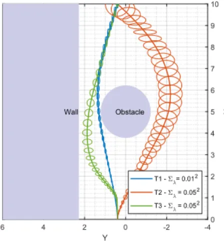
trajectory as the line joining initial to the terminal point for two situations Σλ ={0.012,0.052}. We run the algorithm for following cost functions 1) control effort i.e.,R=Iand Qf =Q= 0 as the cost function forΣλ ={0.012,0.052} shown in Fig. 1 as trajectories T1 and T2 respectively, 2) both control and state penalized in the cost function i.e., R =I andQ=IforΣλ= 0.052shown as trajectory T3 in Fig. 1.
0 1 2 3 4 5 6 7 8 9 10 X -4 -2 0 2 4 6 Y Wall Obstacle T1 - = 0.012 T2 - = 0.052 T3 - = 0.052
Fig. 1: Plot showing mean of the state and uncertainty ellipse corresponding to3σconfidence for = 0.05.
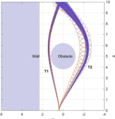
Note that when we minimize both state and control cost we can find a safe trajectory T3 between the wall and the obstacle. The trajectories T1 and T2 were compared in Fig. 2 with the open-loop simulations of the original dynamics in (54) using the policy computed by gPC-SCP approach on the approximated dynamics. Using the open-loop deterministic policy the robot reaches the terminal state with out collision.
Limitations: The Galerkin scheme used in the paper is
computationally expensive, to use the gPC-SCP technique for higher-dimensional problems, numerical methods like stochastic collocation need to be implemented for Galerkin projection. The problem formulation would be same with the stochastic collocation method. The SCP problem requires a good initialization for faster convergence. For longer time
10 9 8 7 6 Wall Obstacle 5 x 4 3 2 '--~~~'--~~~'--~~_.__'--~~~'--~~--' Q 6 4 2 0 -2 -4 y T1 T2
Fig. 2: Plot showing comparison of T1 and T2 trajectories with open-loop policy simulations.
horizon problems multi-element polynomial chaos approach has to be used for uncertainty propagation to achieve better accuracy.
V. CONCLUSION
The paper presented an approximate deterministic surro-gate for the stochastic nonlinear optimal control problem with chance constraints for stochastic trajectory optimization. The approach used generalized polynomial chaos (gPC) to derive a deterministic ordinary differential equation for the stochastic differential equation and a deterministic cost function for the expectation cost function. The main theorem showed that a feasible solution of the deterministic optimal control problem is a feasible solution of the stochastic nonlinear optimal control problem. The proposed gPC-SCP is applied to an example problem to obtain a suboptimal feasible trajectory that is guaranteed to avoid collision with the specified probability. The effectiveness of the method is validated by comparing the trajectories obtained from the method with open-loop runs for multiple realizations of stochastic uncertainty using the open-loop control policy obtained.
ACKNOWLEDGEMENT
This work was in part funded by the Jet Propulsion Labo-ratory, California Institute of Technology and the Raytheon Company.
REFERENCES
[1] LaValle, S. M., Planning Algorithms, Cambridge University Press, 2006.
[2] Spong, M. W., Hutchinson, S., and Vidyasagar, M.,Robot modeling and control, 2006.
[3] Zhou, K., Doyle, J. C., and Glover, K.,Robust and optimal control, Vol. 40, Prentice hall New Jersey, 1996.
[4] Nakka, Y. K., Foust, R. C., Lupu, E. S., Elliott, D. B., Crowell, I. S., Chung, S.-J., and Hadaegh, F. Y., “Six degree-of-freedom spacecraft dynamics simulator for formation control research,”AAS/AIAA Astro-dynamics Specialist Conference, 2018.
[5] Shi, G., Shi, X., O’Connell, M., Yu, R., Azizzadenesheli, K., Anand-kumar, A., Yue, Y., and Chung, S.-J., “Neural lander: Stable drone landing control using learned dynamics,”IEEE International Confer-ence on Robotics and Automation (ICRA), 2019.
[6] Tassa, Y., Mansard, N., and Todorov, E., “Control-limited differential dynamic programming,”IEEE International Conference on Robotics and Automation (ICRA), 2014, pp. 1168–1175.
[7] Todorov, E. and Li, W., “A generalized iterative LQG method for locally-optimal feedback control of constrained nonlinear stochastic systems,” Proceedings of the 2005, American Control Conference, 2005., 2005, pp. 300–306.
[8] Janson, L., Schmerling, E., and Pavone, M., “Monte Carlo motion planning for robot trajectory optimization under uncertainty,”Robotics Research, Springer, 2018, pp. 343–361.
[9] Kushner, H. J., “Numerical methods for stochastic control problems in continuous time,”SIAM Journal on Control and Optimization, Vol. 28, No. 5, 1990, pp. 999–1048.
[10] Kappen, H. J., “Linear theory for control of nonlinear stochastic systems,”Physical review letters, Vol. 95, No. 20, 2005, pp. 200201. [11] Xiu, D. and Karniadakis, G. E., “The Wiener–Askey polynomial chaos for stochastic differential equations,”SIAM journal on scientific computing, Vol. 24, No. 2, 2002, pp. 619–644.
[12] Xiu, D., “Fast numerical methods for stochastic computations: a review,”Communications in computational physics, Vol. 5, No. 2-4, 2009, pp. 242–272.
[13] Calafiore, G. C. and El Ghaoui, L., “On distributionally robust chance-constrained linear programs,” Journal of Optimization Theory and Applications, Vol. 130, No. 1, 2006, pp. 1–22.
[14] Zymler, S., Kuhn, D., and Rustem, B., “Distributionally robust joint chance constraints with second-order moment information,” Mathe-matical Programming, Vol. 137, No. 1-2, 2013, pp. 167–198. [15] Morgan, D., Chung, S.-J., and Hadaegh, F. Y., “Model predictive
con-trol of swarms of spacecraft using sequential convex programming,”
Journal of Guidance, Control, and Dynamics, Vol. 37, No. 6, 2014, pp. 1725–1740.
[16] Morgan, D., Chung, S.-J., and Hadaegh, F., “Spacecraft swarm guidance using a sequence of decentralized convex optimizations,”
AIAA/AAS Astrodynamics Specialist Conference, 2012, p. 4583. [17] Hover, F. S. and Triantafyllou, M. S., “Application of polynomial chaos
in stability and control,”Automatica, Vol. 42, No. 5, 2006, pp. 789– 795.
[18] Fisher, J. and Bhattacharya, R., “Stability Analysis of Stochastic Sys-tems using Polynomial Chaos,”Proc. American Control Conference, 2008, pp. 4250–4255.
[19] Kim, K.-K., Shen, D. E., Nagy, Z. K., and Braatz, R. D., “Wiener’s polynomial chaos for the analysis and control of nonlinear dynami-cal systems with probabilistic uncertainties [historidynami-cal perspectives],”
IEEE Control Systems Magazine, Vol. 33, No. 5, 2013, pp. 58–67. [20] Boutselis, G. I., Pan, Y., De La Tore, G., and Theodorou, E. A.,
“Stochastic trajectory optimization for mechanical systems with para-metric uncertainties,”arXiv preprint arXiv:1705.05506, 2017. [21] Fisher, J. and Bhattacharya, R., “Optimal Trajectory Generation with
Probabilistic System Uncertainty using Polynomial Chaos,”Journal of Dynamic Systems, Measurement, and Control, Vol. 133, No. 1, 2011, pp. 014501.
[22] Blackmore, L., Ono, M., Bektassov, A., and Williams, B. C., “A proba-bilistic particle-control approximation of chance-constrained stochastic predictive control,” IEEE transactions on Robotics, Vol. 26, No. 3, 2010, pp. 502–517.
[23] Blackmore, L., Ono, M., and Williams, B. C., “Chance-constrained optimal path planning with obstacles,”IEEE Transactions on Robotics, Vol. 27, No. 6, 2011, pp. 1080–1094.
[24] Vandenberghe, L., Boyd, S., and Comanor, K., “Generalized Cheby-shev bounds via semidefinite programming,”SIAM review, Vol. 49, No. 1, 2007, pp. 52–64.
[25] Chen, X., “A new generalization of Chebyshev inequality for random vectors,”arXiv preprint arXiv:0707.0805, 2007.
[26] Arnold, L.,Stochastic differential equations, 1974.
[27] Ono, M. and Williams, B. C., “Iterative Risk Allocation: A new approach to robust Model Predictive Control with a joint chance constraint,” 2008 47th IEEE Conference on Decision and Control, Dec 2008, pp. 3427–3432.
[28] Ghanem, R. G. and Spanos, P. D.,Stochastic finite elements: a spectral approach, Courier Corporation, 2003.
[29] Cameron, R. H. and Martin, W. T., “The orthogonal development of non-linear functionals in series of Fourier-Hermite functionals,”Annals of Mathematics, 1947, pp. 385–392.