A new filter QP free method for the nonlinear inequality constrained optimization problem

R E S E A R C H

Open Access

A new filter QP-free method for the

nonlinear inequality constrained

optimization problem

Youlin Shang

_{, Zheng-Fen Jin}

_{and Dingguo Pu}

*_{Correspondence:}

[email protected]

2_{Department of Mathematics,}

Tongji University, Shanghai, China Full list of author information is available at the end of the article

Abstract

In this paper, a filter QP-free infeasible method with nonmonotone line search is proposed for minimizing a smooth optimization problem with smooth inequality constraints. This proposed method is based on the solution of nonsmooth equations, which are obtained by the Lagrangian multiplier method and the function of the nonlinear complementarity problem for the Karush–Kuhn–Tucker optimality conditions. Especially, each iteration of this method can be viewed as a perturbation of a Newton or quasi-Newton iteration on both the primal and dual variables for the solution of the Karush–Kuhn–Tucker optimality conditions. What is more, it is considered to use the function of the nonlinear complementarity problem in the filter, which makes the proposed algorithm avoid the incompatibility. Then the global convergence of the proposed method is given. And under some mild conditions, the superlinear convergence rate can be obtained. Finally, some preliminary numerical results are shown to illustrate that the proposed filter QP-free infeasible method is quite promising.

MSC: 90C20; 90C30; 90C33

Keywords: Nonlinear constrained optimization; Filter method; QP-free method; Nonmonotone line search

1 Introduction

In this paper, we mainly consider solving the nonlinear optimization problem (NLP) with the inequality constraints, where the objective function and the constrained functions are Lipschitz continuously differentiable functions. We give the Lagrangian function associ-ated with this problem, then theKarush–Kuhn–Tucker(KKT) optimality conditions for our solved problem can be obtained.

It is well known that the KKT optimality conditions is a mixed nonlinear complemen-tarity problem (NCP). And this NCP has attracted much attention due to its various ap-plications [1–3] such as the economic equilibrium problem, the restructuring problems of electricity and gas markets, and so on. Of course, there are many efficient methods for solv-ing the NCP, which can be seen in [4–7]. One popular way to solve the NCP is to construct a Newton method for solving the related nonlinear equations, which is a reformulation of the KKT optimality condition. Another way is to use the filter method to directly solve the NLP with the inequality constraints. Recently Pu, Li, and Xue [8] proposed a new quadratic

programming (QP)-free infeasible method for minimizing a smooth function subject to some inequality constraints. This method is based on the solution of nonsmooth equa-tions which are obtained by the multiplier and the Fischer–Burmeister NCP function for the KKT conditions. They proved that the method had a superlinear convergence rate under some mild conditions.

Fletcher and Leyffer [9] proposed a filter method for solving the NLP problem, which was an alternative to the traditional merit functions approach. Provided that there is a sufficient decrease in the objective function or the constraints violation function, it was shown that the trial points generated from solving a sequence of trust region QP subprob-lems are accepted. In addition, the computational results reported in [9,10] are also very encouraging. For more related methods, one can refer to [11–16].

Stimulated by the progress in these two aspects, in this paper, we propose a nonmono-tone filter QP-free infeasible method for minimizing a smooth function subject to smooth inequality constraints. This proposed iterative method is based on the solution of nons-mooth equations, which are obtained by the multiplier and some NCP functions for the KKT first order optimality conditions. And each iteration of this method can be viewed as a perturbation of a Newton or quasi-Newton iteration on both the primal and dual vari-ables for the solution of the KKT optimality conditions. Specifically, we use the filter on the linear search with a nonmonotone acceptance mechanism [17,18]. Moreover, we also consider to use the NCP function in the filter. Thus our algorithm can avoid the incompat-ibility, which may appear in the filter SQP algorithm. We also give the global convergence and the superlinear convergence rate of the proposed method under some mild condi-tions. Finally, we take some numerical tests to illustrate the effectiveness of the proposed filter QP-free infeasible method.

The rest of this paper is organized as follows. In Sect.2, we give some preliminaries and the formulation of the solved problem. Then we propose an infeasible filter QP-free method. In Sect.3, we show that the proposed method is well defined and establish its global convergence and superlinear convergence rate under some mild conditions. Some numerical tests are given in Sect.4. Finally, we give some brief conclusions in Sect.5.

2 Preliminaries and algorithm

In this section, we firstly introduce the formulation of the solved problem. Then we give some preliminaries for structuring a new filter QP-free method. Finally, we present the structure of our proposed method in detail.

In this paper, we mainly consider solving the nonlinear optimization problem (NLP) with the inequality constraints, which can be formulated as

minf(x), s.t. x∈D=x∈Rn|G(x)≤0, (1)

wheref :Rn_{→RandG= (g}

1,g2, . . . ,gm)T:Rn→Rmare Lipschitz continuously differen-tiable functions.

The Lagrangian function associated with problem (1) is

L(x,μ) =f(x) +μTG(x),

Then we can obtain the KKT point (x¯,μ¯)∈Rn_×Rm_{for problem (1), which satisfies the} necessary optimality conditions :

∇xL(x¯,μ¯) = 0, G(x¯)≤0, μ¯≥0, μ¯igi(x¯) = 0, (2)

where 1≤i≤m. We also say thatx¯∈Dis a KKT point of problem (1) if there existsμ¯ ∈Rm such that (x¯,μ¯) satisfies (2). It is well known that the KKT optimality condition is a mixed NCP. And the reformulation of (2) can be viewed as the following nonlinear equation:

(x,μ) = 0.

2.1 Preliminaries

In this subsection, we give the definition of Fischer–Burmeister NCP function and some related Jacobian functions in different cases. Both theoretical results and computational experience have indicated that the nonsmooth methods based on the Fischer–Burmeister NCP function are efficient. The Fischer–Burmeister function has a very simple structure, which is defined as

ψ(a,b) =√a2_+b2_–a–b.

It is clear that this functionψis continuously differentiable everywhere except at the ori-gin, but it is strongly semismooth at the oriori-gin,i.e., ifa= 0 orb= 0, thenψis continuously differentiable at (a,b)∈R2_{, and}

∇ψ(a,b) =

a

√

a2_+b2– 1,

b

√

a2_+b2 – 1

;

ifa= 0 andb= 0, then the generalized Jacobian ofψat (0, 0) is (see [14])

∂ψ(0, 0) =(ξ– 1,η– 1)|ξ2+η2= 1.

Letφi(x,μ) =ψ(–gi(x),μi), 1≤i≤m. Given the above formulation of problem (1), we can denote (x,μ) = ((∇xL(x,μ))T, (1(x,μ))T)T, where 1(x,μ) = (φ1(x,μ), . . . ,

φm(x,μ))T.

Clearly, the KKT optimality conditions (2) can be equivalently reformulated as the non-smooth equations(x,μ) = 0.

If (gi(x),μi)= (0, 0), thenφiis continuously differentiable at (x,μ)∈Rn+m. In this case, we have

∇xφi=

–gi(x)

(gi(x))2+μ2i + 1

∇gi(x); ∇μφi=

μi

(gi(x))2+μ2i – 1

ei,

whereei= (0, . . . , 0, 1, 0, . . . , 0)T∈Rmis theith column of the unit matrix, itsith element is 1, and other elements are 0.

Ifgi(x) = 0 andμi= 0, 1≤i≤m, thenφi(x,μ) is strongly semismooth and directionally differentiable at (x,μ). We have

∂xφi(x,μ) =

and

∂μiφi(x,μ) =

(ξ– 1)|– 1≤ξ≤1.

We may reformulate the KKT at point (x¯,μ¯) conditions as a system of equations:

(x¯,μ¯) =∇xL(x¯,μ¯),1(x¯,μ¯)

= 0,

where μ = (μ1,μ2, . . . ,μm)T ∈ Rm is the multiplier vector, φj(x,μj) = ψ(–gj(x),μj),

1(x¯,μ¯) = (φ1(x¯,μ¯1),φ2(x¯,μ¯2), . . . ,φm(x¯,μ¯m))T. To replace the violation constrained func-tionp(G(x)) in the filterF of Fletcher and Leyffer method [9], we use the violation con-strained functionp(G(x),μ) = 1(x,μ) .

2.2 Algorithm

In this subsection, we give the process and the framework of the filter QP-free method for solving problem (1). We firstly give some closed forms for preparing the method.

If (g(xk_),μk_{)= (0, 0), letξ}k

j =ξj(xk,μk) =

–gk_j

(g_jk)2_+(μk j)2

+ 1;ηk_j =ηj(xk,μk) =

μk_j

(gk_j)2_+(μk j)2

– 1;

otherwise we denoteξ_jk=ξj(xk,μk) = 1 +

√

2/2;ηk_j =ηj(xk,μk) = –1 +

√

2/2. Then let

Vk= V k

11 V12k

V₂₁k V₂₂k

= H

k _∇Gk

diag(ξk)(∇Gk)T diag(ηk–ck)

, (3)

whereHkis a positive matrix, which may be modified by BFGS update. Thediag(ξk) or diag(ηk_–ck_{) denotes the diagonal matrix whosejth diagonal element isξ}k

j orηkj –ckj re-spectively, and

ck_j =cmin1,kν,

wherec> 0 andν> 1 are given parameters.

Secondly, we give the nonmonotone sequence for structuring our method. We may as-sume that the elementskandFkare sorted in the decreasing order, that is,Fˆk1≥ ˆFk2≥

ˆ

Fk3_{≥ · · · ≥ ˆF}kl_,ˆk1_{≥ ˆ}k2_{≥ ˆ}k3_{≥ · · · ≥ ˆ}kl_{. Let}

¯

k== ⎧ ⎨ ⎩

{k_,ˆk2_,ˆk3_{, . . . ,}ˆkl_{}, if} k _<ˆk1_and k _{> 0,}

{ ˆk1,ˆk2,ˆk3, . . . ,ˆkl}, ifk≥ ˆk1ork= 0; (4)

and

¯

Fk== ⎧ ⎨ ⎩

{Fk_,Fˆk2_,Fˆk3_{, . . . ,F}ˆkl_{}, ifF}k_<Fˆk1_, { ˆFk1,Fˆk2,Fˆk3, . . . ,Fˆkl}, ifFk≥ ˆFk1.

(5)

We denote the maximal elements in¯k,F¯k_bypk

max,F¯maxk , respectively.

Algorithm 1NFQPIM

Step 0. Initialization.Given an initial guessx0∈Rn,τ ∈(0, 1),μ¯> 0, 0 <θ1 <θ1< 1, and

a positive definite matrixH0_{. Given initial (f(x}0_),μ¯)∈F0_{. Letp}0

max={Kp,Kp·Kp},F¯max0 =

{Kf,Kf·Kf}andk= 0, whereKp> 0 andKf> 0 are sufficiently large constant numbers.

Step 1. Computation of the search direction.

Ifk= 0, then computedk0andλ¯k0by solving the following linear system in (d,λ):

Vk d

λ

= –∇f

k

0

. (6)

Ifη_jk= 0, then letλk_j0=ηk_jλ¯k_j0/(–ηk_j +ck_j), otherwise letλk_j0=λ¯_jk0. Computedk1_andλ¯k1_by

solving the following linear system in (d,λ):

Vk d

λ

= –∇L k

–k₁

. (7)

Ifηk_j = 0, then letλ_jk1=ηk_jλ¯k_j1/(–η_jk+ck_j), otherwise letλ_jk1=λ¯k_j1.

Step 2. Line search with filter. 1)If

xk+dk1,μk+λk12≤θ1k 2

, (8)

and (9) or (10), at least one holds, then letxk+1_=xk_+dk1_{and =μ}k+1_+λk1_{, go to Step 3.} 2)Line research:

Findxk+1_andμk+1_{to be acceptable for the filter test: letx¯}k+1_=xk_+α

kdk0,μ¯k+1=μk+αkλk0,

ˆ

xk+1_=xk_+α

kdk1, andμˆk+1=μk+αkλk1, whereαk=τjandjis the smallest nonnegative integer satisfying either

1

ˆ

xk+1,μˆk+1≤θ1max1

xk,μkpjmax

(9)

or

fx¯k+1–maxfk,F¯maxj

≤–αkθ1k1+1 (10)

for all (f(xj_), j

1 2)∈Fk. If (9) holds, thenxk+1=xˆk+1,μk+1=μˆk+1 and call it-step; if

(10) holds, thenxk+1_=x¯k+1_,μk+1_=μ¯k+1_{and call itf-step.}

If there are no suchxk+1andμk+1orαktoo small, we use the backtracking technology or use the feasibility restoration phase to findxk+1_andμk+1_{so that it is an acceptable filter}

and theQP(xk+1_{) subproblem is compatible. Go to Step 1.} Step 3. Update.

Ifxk+1_{is a KKT point, then stop, otherwise ifμ}k+1

i ≤ ¯μ, thenμki+1=μki+1; otherwise let

μk_i+1=μ¯, giveHk+1by BFGS update,f¯k+1= 1/2(¯fk+fk+1),Fk+1=Fk∪(f¯(xk+1), k₁ ) and delete all pairs (f¯(xl_), l

1 ) which are dominated by (F(xk+1),μk+1) inFk+1, obtainFk+1.

Remark1 Let(x,μ) = ((∇xL,H(x)), (1(x,μ))T)T, the above proposed NFQPIM can also

be used to solve the following constrained NLP:

min f(x)

s.t. G(x)≤0, H(x) = 0, x∈Rn,

wheref :Rn_{→RandG(x) = (g}

1(x),g2(x), . . . ,gm(x))T:Rn→Rm andH(x) = (h1(x),h2(x),

. . . ,hp(x))T:Rp→Rmare Lipschitz continuously differentiable functions.

2.3 Implementation

In this subsection, we give the implementation of the proposed NFQPIM. Firstly, we sup-pose that the following assumptions A1–A3 hold.

A1. The level set {x|f(x) ≤ f(x0)} is bounded, and for sufficiently large k,

μk_+λk0_+λk1 _<μ¯.

A2. f andgiare Lipschitz continuously differentiable, and for ally,z∈Rn+m,

_∇L(y) –∇L(z)≤m0 y–z , (y) –(z)≤m0 y–z ,

wherem0> 0is the Lipschitz constant.

A3. Hk _{is positive definite and there exist positive numbers m}

1 and m2 such that

m1 d 2≤dTHkd≤m2 d 2for alld∈Rnand allk.

Lemma 1 Ifk_{= 0,then V}k_{is nonsingular.}

Proof Assumek_{= 0. IfV}k_{(u,v) = 0 for some (u,v)∈R}n+m_{, whereu= (u}

1, . . . ,un)T,v= (v1, . . . ,vm)T, then

Hku+∇Gkv= 0 (11)

and

diagξk∇GkTu+diagηk–ckv= 0. (12)

From the definitions ofξ_jkandηk_j, we know thatξ_jk≥0 andη_jk–ck= 0 for allj. Sodiag(ηk– ck_j) is nonsingular. We have

v= –diagηk–ck–1diagξk∇GkTu. (13)

Taking (13) into (11), we have

uTHku+∇Gkv=uTHku–uT∇Gkdiagξkdiagηk–ck–1∇GkTu= 0.

Lemma 2 dk0_{= 0if and only if∇f}k_{= 0,and d}k0_{= 0impliesλ}¯k0_{= 0andλ}k0_{= 0.}

If(x∗,μ∗)is an accumulation point of{(xk_,μk_{)},then d}∗0_{= 0,and(d}∗0_,λ∗0₎T_{is the} solu-tion of the following equasolu-tions:

V∗ d

λ

= –∇f

∗

0

(14)

and∇L(x∗,μ∗) = 0.

It is clear that the following lemma holds, with reference to [8].

Lemma 3 If dk0_{= 0,then}

dk0THkdk0≤–dk0T∇fk.

Proof (14) implies

Hkdk0+∇Gkλk0= –∇fk, (15)

and

diagξk∇GkTdk0+diagηk–ckλˆk0= 0. (16)

We have

ˆ

λk0= –diagηk–ck–1_diagξk_∇GkT_dk0_{. (17)}

Taking (17) into (15), we have

dk0THkdk0+∇Gkλk0

=dk0THkdk0–dk0T∇Gkdiagξkdiagηk–ck–1∇GkTdk0

= –dk0T∇fk. (18)

(dk0₎T_∇G(xk_)diag(ξk_)(diag(ηk_–ck₎₎–1_(∇Gk₎T_dk0_{≤0 implies}

dk0THkdk0≤–dk0T∇fk. (19)

The lemma holds.

Lemma 4 There exists m3> 0such that,for any0 <t≤1,

1

xk+tdk0,μk+tλk02– 1 2≤m3t2.

Proof Ifk₁= 0, then there existsm4> 0 such that, for any 0 <t≤1,

1

xk+tdk0,μk+tλk02=1

xk+tdk0,μk+tλk0–k₁2≤t2m2₂dk0,λk02.

We define that if (g_ik,μk_i)= (0, 0), then (ξ¯_ik0,η¯k_i0) = (ξ_ik,ηk_i), otherwiseξ¯_ik0(∇gk_i)T_dk0₊ ¯

ηk0

i λki0=φi((xk,μk), (dk0,λk0)), where φi((xk,μk), (dk0,λk0)) is the direction derivative of

φi(x,μ) at (xk,μk) in the direction (dk0,λk0).

Letdiag(ξ¯k0) ordiag(η¯k0) denote the diagonal matrix whosejth diagonal element isξ¯_jk0

orη¯k_j0, respectively. Thenφi(0, 0) = 0 implies

k₁Tdiagξ¯k0∇GkT,diagη¯k0=k₁Tdiagξk∇GkT,diagηk.

Then

k₁+tdiagξ¯k0∇GkTdk0+diagη¯k0λk02

=k₁2+t2 diagξ¯k0∇GkTdk0+diagη¯k0λk0) 2. (20)

It is clear that

1

xk+tdk0,μk+tλk02=k₁2+Ot2.

This lemma holds.

Lemma 5 Ifk₁= 0,then given anyε> 0there is¯t> 0such that,for any0 <t≤ ¯t,

k₁2–1

xk+tdk1,μk+tλk12≥(2 –ε)tk₁2.

Proof Ifk₁= 0, (7) implies

diagξk∇GkTdk1+diagηk–ckλk1= –k₁. (21)

We define that if (g_ik,μk_i)= (0, 0) then (ξ¯_ik1,η¯_ik1) = (ξ_ik,η_ik), otherwise (ξ¯_ik1∇g_ik,η¯k_i1)(dk1_,

λk1_{) =φ}

i((xk,μk), (dk1,λk1)), where φi((xk,μk), (dk1,λk1)) is the direction derivative of

φi(x,μ) at (xk,μk) in the direction (dk1,λk1). Letdiag(ξ¯k1) ordiag(η¯k1) denote the diag-onal matrix whoseith diagonal element isξ¯_ik1orη¯_ik1, respectively. Clearly, for alli,

φi

xk+tdk1,μk+tλk1–φ_ik≤tξ¯_ik1∇g_ikTdk1+η¯k_i1. (22)

Sinceck

i = 0, it follows by the definitions ofcki andηki thatηki = 0,gik= 0,μki ≥0, and

φ_ik= 0. We have

k₁+tdiagξ¯k1∇GkTdk1+diagη¯k1λk12

= (1 – 2t)k₁2+tdiagξ¯k1∇GkTdk1+diagη¯k1λk12. (23)

It follows from (22) and (23) that, given anyε> 0, there ist¯> 0 such that, for any 0 <t≤ ¯t,

k₁2–1

xk+t2dk1,μk+tλk12≥(2 –ε)tk₁2.

Lemma 6 dk0_{= 0if and only if∇f}k_{= 0,and d}k0_{= 0impliesλ}¯k0_{= 0andλ}k0_{= 0.}

Proof If∇fk_{= 0, then (x}k_,λ¯k0_{) =V}ˆk_{(0, 0) = (0, 0). Ifd}k0_{= 0, then (14) implies}

diagξk∇GkTdk0+diagηk–ckλ¯k0=diagηk–ckλ¯k0= 0. (24)

Clearly,λ¯k0= 0,λk0= 0, and (∇fk, 0) = (Vk)–1(0, 0) = (0, 0).

From Lemmas3–6, we know that, ifk₁= 0, then (dk_,λk_{) is the decreasing direction of}

k ; ifdk0_{= 0, thend}k_{is the decreasing direction off}k_{. If}k

1= 0 anddk0= 0, then (xk,μk)

is a KKT point. We consider four cases for linear searches. Case 1.k–1 iteration has a-step andk₁= 0. In this case,pk

max=pkmax–1andmin{pkjmax|j∈ Fk_{> 0}. Clearly, we can findα}

ksuch thatxˆk+1satisfies (9).

Case 2.k– 1 iteration has a-step andk₁= 0. In this case, it follows from Lemma5

that, given anyε> 0, there is¯t> 0 such that, for any 0 <t≤ ¯t,

k₁2–1

xk+tdk1,μk+tλk12≥(2 –ε)tk₁2.

pk

max> 0 is monotonically nonincreasing. So, we can findαksuch thatxˆk+1satisfies (9). Case 3.k– 1 iteration has anf-step anddk0_{= 0. In this case, it follows from Lemma5}

that, ifdk0_{= 0, then}

dk0THkdk0≤–dk0T∇fk,

where fmaxk is monotonically nonincreasing. We can find αk such that x¯k+1 satisfies (10).

Case 4. The (k– 1) iteration has anf-step anddk0= 0. In this case, ifk₁= 0, then (xk,μk) is a KKT point, otherwisexk_{may be an infeasible stationary point.}

If there are no suchxk+1andμk+1orαktoo small, we use the backtracking technology or use the feasibility restoration phase to findxk+1_andμk+1_{so that it is acceptable that the}

filter and theQP(xk+1) subproblem are compatible.

3 Convergence

In this section, we discuss the global and superlinear convergence rate of the proposed method. We give the following A4 and suppose that the assumptions A1–A4 hold in this section.

A4. For allkand someαmin> 0,αk>αmin> 0. It implies from (3) and (4) that pk

max > 0 is monotonically nonincreasing and, if

1(xk) →0, thenpkmax→0.

Lemma 7 Consider the sequence{ 1(xk) 2}and{fk}such that{ 1(xk) 2≥0}and{fk}

is monotonically decreasing and bounded below.Let a constantθsatisfy,for all k and l∈Fk, that

1

ˆ

xk+1,μˆk+1≤θ1max1

xk,μkpjmax

or

fx¯k+1–maxfk,F¯maxj

≤–αkθ1k1+1, (26)

whereαk≥αmin> 0is the step length,θ is a given positive number.Then pkmax→0.

Proof Suppose that the theorem is not true, then1(xk)→0, and there existε> 0 and

infinitely many members of index setKsuch that 1(xk+1,μk+1) ≥ε> 0,pkmax≥ε> 0, and 1(xk+1,μk+1) ≥θ 1(xk,μk) for anyk∈K. We have

fxk–fxk+1≥αkθ1

xk+1,μk+1>αminθ ε. (27)

Because{fk_{}is monotonically decreasing, (27) impliesf(x}k_{)→–∞ask→+∞, which is} contravention of{fk_{}being bounded below. This lemma holds.}

Lemma 8 Consider an infinite sequence iterations on which{fk_,

1(xk) 2}entered into

the filter,where 1(xk) > 0and{fk}is bounded below.It follows that1(xk)→0.

Theorem 1 If(x∗,μ∗)is an accumulation point of{(xk_,μk_{)},then x}∗ _{is a KKT point of} problem(1).

Proof It is obvious that Lemmas8and2imply that Theorem1holds.

Next we consider the superlinear convergence of the method and firstly give the follow-ing assumptions we need.

A5. The Mangasarian–Fromovitz (M-F) qualification condition is satisfied atx∗, i.e., {∇gi(x∗)}are linear independent for alli∈I={i|gi(x∗) = 0}, and there exists a

direc-tion such thatdT_∇g

i(x∗) < 0,i∈I={i|gi(x∗) = 0}, wherei∈I={i|gi(x∗) = 0}, where x∗is an accumulation point of{xk_{}and a KKT point of problem (1).}

A6. The sequence of{Hk_}satisfies

(Hk_–∇2

xL(xk,μk))dk1

dk1 →0.

A7. The strict complementarity condition holds at each KKT point(x∗,μ∗).

It follows thatφk_{is differentiable at each KKT point (x}∗_,μ∗_).

Assumption A7 implies thatis continuously differentiable at each KKT point (x∗,μ∗). As Lemma1, we have that the following lemmas hold.

Lemma 9 AssumeA1–A7hold,then{ (Vk₎–1 _{}and{ (V}ˆk₎–1 _{}are bounded.}

Further-more,if V∗is an accumulation matrix of{Vk_{},then V}∗_{is nonsingular.}

Proof By Theorem1,∗= 0 andck_{→0. Without loss of generality, we may assume that} (xk_,μk_)→(x∗_,μ∗_),Hk_→H∗_,diag(ξk_)→diag(ξ∗_{), anddiag(η}k_)→diag(η∗_{). By the} defi-nitions ofξ_ikandηk_i, we know that (ξ_i∗)2_{+ (η}∗

If V∗(u,v) = 0, where (u,v)∈Rn+m _andu={(u

1, . . . ,un)T},v={(v1, . . . ,vm)T}, then we have

H∗u+∇G∗v= 0 (28)

and

diagξ∗∇G∗Tu+diagη∗v= 0. (29)

From (29) and the definitions ofξ_j∗andη∗_j, we know that ifξ_j∗= 0 thenη_j∗= 0. Ifξ_j∗= 0 then

uT∇g_j∗= –η ∗ j

ξ_j∗vj. (30)

Putting (29) and (30) into (28), we have

uTH∗u+∇G∗v

=uTH∗u+ j:ξ_j∗=0

–η ∗ j

ξ_j∗v

2

j = 0. (31)

η∗_j/ξ_j∗≤0 impliesu= 0, and ifη_j∗= 0 thenvj= 0. LetI={j|gj∗= 0}, becauseg∗j = 0 implies

η∗_j = 0 andvj= 0, we have

j∈I

∇g_j∗vj= 0, (32)

andvj= 0 (j∈I) by A4,i.e., (u,v) = 0 andV∗is nonsingular.

On the other hand, suppose to the contrary that there exists a subsequence{(xk(i)_,λk(i)_)}

such that (Vk(i)₎–1 _{→ ∞ask(i)→ ∞and (x}k(i)_,λk(i)_)→(x∗_,λ∗_{). We can choose k(i)} properly such thatVk(i)→V∗includingξk(i)→ξ∗andηk(i)→η∗. Clearly, (ξ_j∗)2+ (η∗_j)2≥ 3 – 2√2 > 0 andV∗∈∂∗. But V∗ is nonsingular by the above proof, which contra-dicts the assumption (Vk(i)₎–1 _{→ ∞. Hence,{ (V}k(i)₎–1 _{}is bounded.}k_{→0 implies}

limk→∞Vk =limk→∞Vˆk, we can also obtain that { (Vˆk)–1 }is bounded. This lemma

holds.

Assumption A5 shows that (xk_,μk_{) is a Newton direction with a high order perturbation.} We obtain the following lemma.

Lemma 10 For sufficiently large k,xk+1_=xk_+dk1_andμk+1_=μk_+λk1_.

Furthermore, Lemma10implies that the following theorem holds.

4 Numerical tests

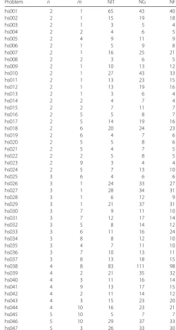
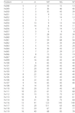
We use Algorithm1(NFQPIM) for the constrained optimization problems (see [19]):Hk is updated by the BFGS method. The termination criterion is φ ≤10–5_{. The parameters}

are chosen as follows:c= 0.1,ν= 2,τ= 0.7,θ1= 0.8,θ= 0.6,μ¯ = 10,000. In the “NIT/NG”

entry of the table below, NIT is the number of iterations, NF represents the number of function evaluations, NG denotes the number of gradient evaluations. The numerical re-sults can be seen in the Table1. We test the proposed NFQPIM for solving almost 100 optimization problems. And the numerical results illustrate that the proposed method is efficient and promising.

Table 1 Numerical results on the NFQPIM for some constrained optimization problems

Problem n m NIT NG NF

hs001 2 1 65 43 40

hs002 2 1 15 19 18

hs003 2 1 3 5 4

hs004 2 2 4 6 5

hs005 2 4 9 11 9

hs006 2 1 5 9 8

hs007 2 1 16 25 21

hs008 2 2 3 6 5

hs009 2 1 10 13 12

hs010 2 1 27 43 33

hs011 2 1 13 23 15

hs012 2 1 13 19 16

hs013 2 1 3 6 4

hs014 2 2 4 7 4

hs015 2 2 7 11 7

hs016 2 5 5 8 7

hs017 2 5 14 19 16

hs018 2 6 20 24 23

hs019 2 6 4 7 6

hs020 2 5 5 8 6

hs021 2 5 4 7 5

hs022 2 2 5 8 5

hs023 2 9 3 4 4

hs024 2 5 7 13 10

hs025 3 6 4 6 6

hs026 3 1 24 33 27

hs027 3 1 28 34 31

hs028 3 1 6 12 9

hs029 3 1 21 37 31

hs030 3 7 9 11 10

hs031 3 7 12 17 14

hs032 3 5 8 14 12

hs033 3 6 11 16 24

hs034 3 8 8 12 10

hs035 3 4 7 11 10

hs036 3 7 10 13 11

hs037 3 8 13 18 15

hs038 4 8 83 111 98

hs039 4 2 21 35 32

hs040 4 3 11 16 14

hs041 4 9 13 17 15

hs042 4 2 11 14 12

hs043 4 3 15 23 20

hs044 4 10 16 23 21

hs045 5 10 5 7 7

hs046 5 10 29 37 33

Table 1 (Continued)

Problem n m NIT NG NF

hs048 5 2 10 15 13

hs049 5 2 36 46 40

hs050 5 3 35 43 39

hs051 5 3 9 13 11

hs052 5 3 7 14 12

hs053 5 3 5 7 7

hs054 6 13 9 13 10

hs055 6 14 8 14 11

hs056 7 4 12 14 12

hs057 2 3 6 9 8

hs059 2 7 28 33 30

hs060 3 7 13 23 21

hs061 3 2 59 68 58

hs062 3 7 24 33 28

hs063 3 5 15 23 20

hs064 3 4 36 43 37

hs065 3 7 21 29 27

hs066 3 8 13 23 19

hs067 3 41 65 53 47

hs099 7 16 65 43 40

hs100 7 4 65 43 40

hs101 7 20 65 43 40

hs102 7 20 65 43 40

hs103 7 20 65 43 40

hs104 8 22 65 43 40

hs105 8 17 65 43 40

hs106 8 22 65 43 40

hs107 9 14 65 43 40

hs108 9 14 33 30

hs110 10 20 25 43 40

hs111 10 23 61 73 68

hs112 10 13 51 73 67

hs113 10 8 55 65 61

hs114 10 31 56 73 68

hs116 13 41 123 143 140

hs117 15 20 511 63 60

hs118 15 59 67 81 77

hs119 16 40 68 83 78

5 Conclusions

In this paper, we developed a nonmonotone filter QP-free infeasible method for minimiz-ing a smooth optimization problem with inequality constraints. This proposed method is based on the solution of nonsmooth equations which are obtained by the multiplier and some NCP functions for the KKT first-order optimality conditions. At each iteration of the proposed method, it was a perturbation of a Newton or quasi-Newton iteration on both the primal and dual variables for the solution of the KKT optimality conditions. More-over, we used the filter on linear searches with a nonmonotone acceptance mechanism. We also showed that the proposed method had a global convergence and a superlinear convergence rate. Finally, the numerical results illustrated that the proposed method was efficient. However, how to apply this method to the real optimal problem will be studied in the near future.

Acknowledgements

Funding

The work of Y. Shang is supported by the National Natural Science Foundation of China Grant No.11471102. The work of D. Pu is supported by the National Natural Science Foundation of China Grant No. 11371281. The work of Z.-F. Jin is supported by the National Natural Science Foundation of China Grant No. 61772174, Plan for Scientific Innovation Talent of Henan Province Grant No. 174200510011.

Competing interests

The authors declare that they have no competing interests.

Authors’ contributions

All authors contributed equally to this work. All authors read and approved the final manuscript.

Author details

1_{School of Mathematics and Statistics, Henan University of Science and Technology, Luoyang, China.}2_{Department of}

Mathematics, Tongji University, Shanghai, China.

Publisher’s Note

Springer Nature remains neutral with regard to jurisdictional claims in published maps and institutional affiliations.

Received: 18 April 2018 Accepted: 12 September 2018 References

1. Chen, X.: Smoothing methods for complementarity problems and their applications: a survey. J. Oper. Res. Soc. Jpn.

43, 32–47 (2000)

2. Arrow, K.J., Debreu, G.: Existence of an equilibrium for a competitive economy. Econometrica,22, 265–290 (1954) 3. Smeers, Y.: Computable equilibrium models and the restructuring of the European electricity and gas markets.

Energy J.0(4), 1–31 (1997)

4. Tian, B., Yang, X.: Smoothing power penalty method for nonlinear complementarity problems. Pac. J. Optim.12(2), 461–484 (2016)

5. Xie, S.L., Xu, H.R., Zeng, J.P.: Two-step modulus-based matrix splitting iteration method for a class of nonlinear complementarity problems. Linear Algebra Appl.494, 1–10 (2016)

6. Otero, R.G., Iusem, A.: A proximal method with logarithmic barrier for nonlinear complementarity problems. J. Glob. Optim.64(4), 663–678 (2016)

7. Hao, Z., Wan, Z., Chi, X., Chen, J.: A power penalty method for second-order cone nonlinear complementarity problems. J. Comput. Appl. Math.290, 136–149 (2015)

8. Pu, D.G., Li, K.D., Xue, J.: Convergence of QP-free infeasible methods for nonlinear inequality constrained optimization problems. Tongji Daxue Xuebao Ziran Kexue Ban33, 525–529 (2005)

9. Fletcher, R., Leyffer, S., Toint, P.: On the global convergence of a filter-SQP algorithm. SIAM J. Optim.13, 44–59 (2002) 10. Ulbrich, M., Ulbrich, S.: Non-monotone trust region methods for nonlinear equality constrained optimization without

a penalty function. Math. Program.95, 103–135 (2003)

11. Yang, Y., Shang, Y.: A new filled function method for unconstrained global optimization. Appl. Math. Comput.173, 501–512 (2006)

12. Qi, H.D., Qi, L.: A new QP-free, globally convergent, locally superlinearly convergent algorithm for inequality constrained optimization. SIAM J. Optim.11, 113–132 (2000)

13. Liu, F.T., Fan, Y.H., Yin, J.H.: The use of QP-free algorithm in the limit analysis of slope stability. J. Comput. Appl. Math.

235, 3889–3897 (2011)

14. Pu, D.G., Zhou, Y., Zhang, H.Y.: A QP free feasible method. J. Comput. Math.22(5) 651–660 (2004)

15. Jian, J.B., Guo, C.H., Tang, C.M., Bai, Y.Q.: A new superlinearly convergent algorithm of combining QP subproblem with system of linear equations for nonlinear optimization. J. Comput. Appl. Math.273, 88–102 (2015)

16. Zhang, H., Li, G., Zhao, H.: A kind of QP-free feasible method. J. Comput. Appl. Math.224, 230–241 (2009)

17. Huang, M., Pu, D.: Line search SQP method with a flexible step acceptance procedure. Appl. Numer. Math.92, 98–110 (2015)

18. Huang, M., Pu, D.: A line search SQP method without a penalty or a filter. Comput. Appl. Math.34, 741–753 (2015) 19. Dolan, E.D., Moré, J.J.: Benchmarking optimization software with performance profiles. Math. Program.91, 201–213