Educational value added and programme evaluation

EDUCATIONAL VALUE ADDED

AND

PROGRAMME EVALUATION

by

DAVID MAYSTON*

University of York

CONTENTS

Executive Summary ... 1

1. Introduction

2. The Value Added Concept ... 9

3. Multilevel Approaches ... 13

4. The Magnitude of the School Effect ... 19

5. Multivariate Approaches ... 23

6. Non-Parametric Approaches ... 29

7. Aggregation Issues ... 39

8. The Explanatory Variables ... 45

9. The Functional Form ... 61

10. Differential School Effectiveness ... 73

11. Measurement Errors and Endogeneity Issues ... 77

12. Programme Evaluation and Comparison Groups ... 89

13. Extensions of the Evaluation ... 107

14. Conclusion ... 121

EXECUTIVE SUMMARY

The evaluation of educational initiatives, such as the Academies programme, raises interesting questions as to the appropriate analytical tools and methodologies to be adopted in the evaluation. In this Research Report, we examine two main literatures which are relevant to this area. The first is the large and growing literature on the assessment of value added in the education sector. The second is the developing literature on programme evaluation in contexts

where the conditions for carrying out randomised control trials (RCTs) are not fulfilled. We

will examine both the opportunities and remaining problems that these approaches present for the evaluation of educational initiatives. In addition, we will seek to bring these two approaches productively together in providing appropriate analytical tools for the evaluation of educational initiatives, whether in a local, national or international context.

The concept of educational value added, and its potential roles in promoting and assessing school effectiveness, are examined in Section 2. Section 3 examines a number of formulations

of the value added model, including the use of multilevel modelling to take into account the

hierarchical structure of pupils being educated within classes within schools. While the

efficiency of the parameter estimates can be improved by adjusting for the heteroscedasticity

which such a hierarchical structure implies, there remain potential problems of instability in

the parameter estimates which the associated Iterative Generalised Least Squares (IGLS)

estimation procedure generates. The magnitude of the estimates of the school effect which

multilevel models generate is examined in Section 4. While estimates of the difference that the school makes range from 1.5 per cent to 25 per cent of the variance explained, most estimates are concentrated around 10 per cent. This itself suggests that differences between schools in general do not make dramatic differences to educational outcomes, once other variables are taken into account. By far the largest part of the variance of individual pupil achievement is that explained by individual pupil prior attainment, underlining the need to make use of value added measures of pupil progress which adjust for this factor.

Section 5 examines a number of multivariate approaches to analysing value added. While the use of Ordinary Least Squares (OLS) multivariate regression analysis on pupil-level data does not produce minimum variance estimates of the relevant parameters, it does nevertheless

produce estimates of the fixed effect coefficients of the model that will be unbiased. The

compared to the use of multilevel error component models, may, however, result in some fixed effect variables being accepted as statistically significant under OLS which would not be found to be so under multilevel modelling. The extent of this under-estimation will tend to be greater,

the greater is the intra-school correlation between the value-added residuals, and the greater

is the number of pupils per school.

However, while the estimates of the fixed effect parameters are unbiased under both multilevel

modelling and OLS, the estimates of the school random effects that indicate individual school

contributions to pupil value added are not unbiased under multilevel modelling. Instead the use

of a ‘shrinkage factor’ in the multilevel estimation procedure to reflect the assumed reliability

of parameter estimates reduces the estimates of school effectiveness, particularly for small schools. Simulation studies show that the use of multilevel models are then not always strongly preferable to the use of OLS on pupil-level data, particularly once possible instabilities in the Iterative Generalised Least Squares (IGLS) procedure of multilevel modelling are taken into account.

Section 6 reviews the use of non-parametric statistics to assess pupil progress and school effectiveness in place of regression-based models of pupil value added. This includes particularly pupil value added computed from a comparison between a pupil’s actual level of performance at GCSE or other Key Stage with the level of performance which would have been predicted for them on the basis of their prior attainment at the previous stage, such as at Key Stage 3 (KS3), using a ‘median curve’. The median curve is mapped out by graphing the

national median level of performance of pupils at the later stage, such as GCSE, amongst

pupils nationally with similar prior attainments at the earlier stage, such as at KS3, against their prior attainment point score. School-level value added is computed by taking the arithmetic average of the pupil-level value-added measures. Studies by the DfES show that the extent of such pupil progress varies according to pupil gender, Free School Meals (FSM) eligibility, and ethnicity, as well as school-level variables, such as the proportion of pupils in the school eligible for FSM and the type of school involved. Systematically taking all of these additional influences into account, and assessing their statistical significance, in estimating the additional contribution which each individual school makes to pupil value added in the presence of variations across schools in these variables is difficult under a non-parametric approach, but remains feasible using a multilevel parametric model.

Section 7 reviews several studies of school value added which disaggregate the analysis to

individual subject areas, and show both variations between schools in their levels of relative

effectiveness across subjects, and also that variables such as pupil gender and pupil social background have a different influence on different subjects, such as English and mathematics.

Other value-added studies have included not only school effects but also teacher and class

effects when an extensive database on these intermediate variables has been available. In

contract to the insights which these disaggregated studies reveal, aggregated single-level studies based upon regressing mean levels of school educational attainment on school mean levels of explanatory variables risk the ‘ecological fallacy’ of misinterpreting the resultant coefficients as confirming a significant relationship at an inappropriate level of the educational process.

Section 8 reviews the large number of studies in England and elsewhere which have examined

the influence of additional explanatory variables in explaining pupil value added. These

include not only pupil gender, but also pupil background variables that may reflect

socio-economic disadvantage or initial difficulties when English is not the pupil’s first language or

a continuing influence of the pupil’s junior school. In addition, they include school context

variables which may reflect peer group pressures and wider social influences. The DfES’s

recent development of Contextual Value Added (CVA) models that incorporate many school- and pupil-level contextual variables using multilevel modelling, into the analysis of value added in different subjects at different stages of the educational process, represents a significant advance over earlier non-parametric methodology that did not take these variables systematically into account.

Section 8 also reviews other studies which have included school resources and school

processes, and those which have examined the stability over time in annual estimates of

individual school effectiveness. These have found positive, though imperfect, correlations over time in these annual estimates of school effectiveness, with different relative rates of individual

school improvement or deterioration and some evidence of changes in the relative efficiency

of different schools.

Different possible choices of the functional form for the value-added equation, and associated

choice of transformation of the variables, are reviewed in Section 9. The merits of the

the educational production function, or a translog flexible functional form or a semi-log or logarithmic-reciprocal model. Rather than simply regarding the school effect disturbance term as an indicator of school effectiveness in a given single direction of educational attainment,

stochastic frontier analysis seeks to distinguish such effectiveness from heterogeneity of the

position of the underlying production frontier for each school due to additional unobserved

factors. In contrast, Data Envelopment Analysis (DEA) adopts a non-stochastic approach to

estimating a common production frontier for all schools that can take into account the multiple outputs which the school produces in different subjects and at different stages of the

educational process. However, the coefficient of technical efficiency which DEA estimates for

each school in this multiple output context does not itself provide detailed information on the effectiveness of the school in each relevant direction of educational attainment.

Section 10 examines extensive empirical studies which have been carried out into the possible

existence of differential slope parameters on pupil prior attainment across different schools.

Incorporating such a possibility through a random coefficients model allows greater

consideration to be given to issues of equality of treatment and of educational effectiveness

across different ability groups within the school. Mixed empirical evidence has been found in

this context, though with differentiation by subject again showing interesting variations in school effectiveness. Other studies of differential school effectiveness have investigated the

possibility of differential school effectiveness for different pupil groups differentiated by

gender, ethnicity, FSM status or social class.

Section 11 examines several sources of possible endogeneity bias which may cause the

Section 11 also examines the possible influence of measurement errors in biasing the

estimated coefficients in a value-added analysis away from their true value in an underlying educational production function. However, knowledge of the true values in an underlying educational production function becomes less critical when value-added analysis is itself defined in terms of a comparison between achieved levels of pupil attainment and their

predicted levels, conditional on the observed values of the explanatory variables.

Nevertheless, there is a need for further research into the sensitivity of estimates of pupil- and

school-level value added to possible variations in the observed data within the range of their likely inaccuracies, and the extent to which increasing the number of explanatory variables,

rather than greater parsimony in their selection, reduces the robustness of the estimates to

departures from the underlying assumptions of the model.

The developing literature on techniques of programme evaluation in conditions where

randomised control trials are not feasible is examined in Section 12. In the absence of a

random allocation of schools and pupils to the programme under a controlled experimental

design, selection bias may arise that can bias the estimates of the programme impact that are

generated by a technique such as multilevel modelling. The merits of other techniques, such as

difference-in-differences estimators, are discussed, both in the context of a homogeneous

(i.e. uniform) impact of the Academies programme on all schools participating in the

programme and in the context of a heterogeneous programme impact. Section 12 also

reviews the assumptions and implications of techniques of matching, such as the use of

Propensity Score Matching under which schools would be matched that had the same

probability of being selected for the Academies programme. In addition, the formulation of

relevant comparison groups is discussed in Section 12. An important common feature of

schools in the Academies programme is their low average level of pupil prior attainment at

KS2, which, in line with value-added analysis, can be used as a key criterion to define relevant comparison groups.

A technique that has scope for application in the evaluation of the impact of the Academies when school- and pupil-level data are available both before and after the start of the

programme is the use of a regression-adjusted conditional difference-in-differences

matching estimator. This can generate consistent estimates of the programme impact under

considerably weaker assumptions than those which are required under Propensity Score

effectiveness, both before and after the programme has been in operation, for both Academy schools, and their predecessor schools, and for schools in the comparison group. By adjusting measures of pupil attainment, such as examination results, for pupil prior attainment and other relevant pupil- and school-level variables, value-added analysis not only isolates more closely the contribution which the individual school makes to the pupil’s educational progress, but at the same time corrects for many of the factors which would otherwise bias estimates of the impact which participation in an educational initiative, such as the Academies programme, has on those schools in the programme.

Several extensions to the application of relevant difference-in-differences techniques to the evaluation of the Academies programme are discussed in Section 13. These extensions include

examining the impact of the programme on disaggregated measures of examination

performance at different stages of the educational process and in different subjects, on attendance and exclusions, and on the characteristics of their pupil intake. In addition, they

include examining the impact of the programme on other secondary schools and on their

Primary Feeder schools.

1. INTRODUCTION

The evaluation of educational initiatives, such as the Academies programme, raises interesting questions as to the appropriate analytical tools and methodologies to be adopted in the evaluation. In this Research Report, we examine two main literatures which are relevant to this area. The first is the large and growing literature on the assessment of value added in the education sector. The second is the developing literature on programme evaluation in contexts where the conditions for carrying out randomised control trials (RCTs) are not fulfilled. We will examine both the opportunities and remaining problems that these approaches present for the evaluation of educational initiatives. In addition, we will seek to bring these two approaches productively together in providing appropriate analytical tools for the evaluation of educational initiatives, whether in a local, national or international context.

This review examines firstly the main approaches, conclusions, and issues of continued debate, associated with the current literature on the concept and measurement of value added in education, and especially in secondary education. Value added in its general economic sense refers to the extent to which the value of the inputs into the production process is increased when these inputs are transformed into the outputs of the production process. The concept of value added, or ‘added value’, is defined by Kay (1993) as “the difference between the (comprehensively accounted) value of a firm’s output and the (comprehensively accounted) cost of the firm’s inputs”, arguing that “In this specific sense, adding value is both the proper motivation of corporate activity and the measure of its achievement”. The computation of value added in this and related contexts, such as the assessment and administration of Value Added Tax, makes use of market prices to assess the value of inputs and outputs. However, many of the inputs and outputs of education have no simple market value. In the case of education, the inputs into the production process include not only resource inputs, but also pupils with different individual characteristics who do not have a direct market value.

While the concept of human capital (Becker, 1993) has been complemented by the computation of labour market rates of return on some stages of the educational process (see

e.g. Dearden et al, 2000) and on studying some subjects, such as A-level mathematics (Dolton

2. THE VALUE ADDED CONCEPT

The broader economic issues are to some extent side-stepped by the more specific interpretation which has been given in recent years to the concept of value added in assessing performance within the education sector. This interpretation relates to the extent to which the pupils who are the subject of the value-added analysis are achieving the levels of educational

performance that might be predicted for them at a given stage of the educational process,

based upon information on their educational attainments at an earlier stage of the educational

process, and upon other information that is considered relevant. For any given cohort Cjg of

pupils in school j at stage g of the educational process, this gives a definition of their educational value added as:

[ ( , , )]

jg

Cjg ijg ijg ijg r ijg j i C

v q P q q x s

ε −

=

∑

where qijg is a measure of the educational attainment of pupil i in school j at stage g of the

educational process, P(qijg⏐qijg-r, xijg, sj) denotes the predicted value of qijg conditional on the

prior attainment qijg-1 of pupil i in school j at a previous stage g-r of the educational process,

xijg is a vector of other pupil characteristics that are considered to have an influence on the

pupil’s educational progress, and sj is a vector of school-level variables that are considered

relevant to the analysis.

A frequent means of deriving the predicted value, P(qijg⏐qijg-r, xijg, sj), is the use of regression

analysis, in one of several different forms discussed below. The value added for each

individual pupil is then the difference between their actual educational attainment score and

that predicted for them, given qijg-r, xijg and sj, by the regression line based upon a wider sample

of pupils and/or schools. The definition of value added is therefore a relative one, of how well

the pupils have progressed compared to what can be predicted or expected for them, given their prior attainment qijg-r, their other individual characteristics xijg and the school-level variables sj,

on the basis of a regression analysis of data on individual pupil achievements, qijg , and on qijg-r,

xijg and sj for pupils drawn from a wider sample of pupils and schools. The sum of the value-

added measures for all the relevant pupils in the school yields the value-added score for the

school as a whole in (2.1), when Cjg is taken to refer to all the pupils who have completed stage

the school, the total value-added measure for the school may be divided by the number of pupils in the school who have completed stage g of the educational process in the school at the relevant date, to yield their average value added. A school will achieve a larger value-added score if the computed residual values of its individual pupil attainments at stage g, when compared to those that are predicted by the regression line, are greater. Such an outcome would be achieved, for example, by ensuring that their pupil achievements at stage g are all a larger distance above the predictive regression line. This basic approach is therefore referred to as

Residual Gain Analysis by Fitz-Gibbon (1995).

The main roles which the value added concept is seeking to fulfil relate particularly to the

assessment, and possible improvement, of school effectiveness. These potential roles include

those of:

i. providing useful information to the management of each school on their performance relative

to other schools in similar circumstances;

ii. providing information to parents on the school’s educational effectiveness; and

iii. providing information to the wider public on the relative performance of the school to

promote public accountability.

Much of the interest in school value-added measures in this context has arisen as a reaction to the perceived deficiencies of unadjusted school league tables that followed the requirement of the 1980 Education Act for secondary schools in England to publish their examination results.

These presented summary measures of pupil achievements, qijg, within the school without

making any allowances for differences in pupil prior attainment levels or in other variables

within the vectors xijg and sj that might be considered relevant in a value-added analysis. In

contrast, a value-added approach to the assessment of school effectiveness implicitly regards the role of the school as adding value to pupils, who may start from different levels of prior attainment and have other relevant characteristics, that may influence their ability to achieve different levels of performance at the end of the given stage of the educational process.

account. Schools that serve pupils from disadvantaged backgrounds, but who none the less succeed in achieving examination results that are significantly higher than would be predicted for such a group of pupils, may then be judged as very effective under a value-added approach, but might be unfairly judged as ineffective if only their unadjusted position in school league tables was taken into account without regard to their disadvantaged pupil intake. In response to such criticism of unadjusted school examination results, the Dearing Report (1993) recommended the publication also of school value-added information as “a valuable contribution to appraising performance and to improving accountability”.

A further important role for value-added analysis in the context of the Academies programme is:

iv. assessing the extent to which programme participation and changes in school status succeed

in boosting the effectiveness of the schools concerned.

Because they are located in areas of social disadvantage, a value-added analysis approach has

clear attractions in addressing the issues which are involved in this assessment. Since iv. in

particular involves progress, and potential improvements in value added, over time, it is

important that the value-added framework adopted can compare changes in value added over time in the Academies with the extent of the improvements which are taking place over the

same period of time in appropriate comparison groups of schools. We will return in Section

3. MULTILEVEL APPROACHES

Performance data on pupils have a natural hierarchical structure in which pupils are located

within classes within schools, that are in turn located within LEAs. Within this hierarchical structure, Aitken and Longford (1986) considered a number of formulations of the basic model for assessing school effectiveness under a value-added approach. The first was of the form:

qij = α + βx1ij + γx2ij + εij for i = 1, ..., nj ; j = 1,...,m (3.1)

where qij denotes the level of attainment of pupil i in school j at the end of the relevant phase

of education, such as a Key Stage, x1ij denotes the level of prior attainment of the pupil at the

start of the relevant phase of education, x1ij is an additional pupil-level variable of interest, such

as the gender or socio-economic background of the pupil, and εij is a stochastic disturbance

term that is assumed to be normally distributed with mean zero and a variance of σ2_{. m is the}

number of schools in the analysis and nj is the number of pupils in school j. α, β and γ are

constant parameters to be estimated here using Ordinary Least Squares (OLS) regression

analysis. An estimate of a ‘school effect’ or ‘coefficient of school value added’ can be

obtained from the mean across pupils in the school of the residuals from an OLS regression, to

obtain the predicted value of qij,, given the pupil’s prior attainment level, x1ij , and the value of

the variable x2ij , for each school j and pupil i. A model of the form of (3.1) was deployed in the

U.S. Coleman (1996) report, which concluded that “schools are remarkably similar in the way they relate to the achievement of their pupils when the socioeconomic background of the students is taken into account ... it appears that differences between schools account for only a

small fraction of differences in pupil achievement” (ibid, pp. 21-22).

One of the assumptions of the standard OLS regression model (see e.g Gujarati, 1995) applied

to (3.1) is that the variance of the stochastic disturbance term εij for each given value of x1ij

and x2ij is the same constant, σ2 . However, as Goldstein (1987, 1995) has stressed, the

variance of distribution of εij may well vary from school to school, with some schools facing

more pupil-level variation than others. Such a variation in the pupil-level variance will

introduce into (3.1) a element of heteroscedasticity. While they are still unbiased estimates if

regression coefficients α, β and γ will then not be efficient, i.e. minimum variance estimates

in the class of linear unbiased estimators.

A second basic formulation of the value-added model of school effectiveness is that of:

qij = αj + βx1ij + γx2ij + εij for i = 1, ..., nj ; j = 1,...,m (3.2)

where (3.2) replaces the constant intercept term α in (3.1) with a school-specific intercept term

αj to define a school fixed effect that represents the contribution of school i to pupil value

added. (3.2) describes a set of parallel school-specific regression lines which differ from each

other by variations in the extent of their school-specific intercept term αj . The relative

value-added by school j can now be computed as the value of αj compared to the mean value of these

school intercept terms across all schools. Due to the continued problem of heteroscedasticity,

the parameter estimates for αj , β and γ will still be subject to large standard errors if OLS

is used for their estimation.

A third possible formulation which has been used in the literature on assessing school effectiveness, as in Marks, Cox and Pomian-Srzednicki (1983), is that of Aitken and Longford

(1986)’s Model 3, involving the school-level mean value of pupil achievement, Qj , for each

school j together with the school-level mean values, X1j and X2j , of the pupil prior attainment

levels and additional explanatory variable for school j, i.e.

Qj = α + βX1j + γX2j + ηj for j = 1,...,m (3.3)

where ηj is a school-level disturbance term. If a form of weighted least squares is used to

estimate the parameters of (3.3), the parameter estimates for β on pupil prior attainment in

(3.1), (3.2) and (3.3) will in general differ according to the extent to which pupil-level

variations in prior attainment level are due to within-school variations or across-school

variations. This extent is itself likely to depend upon the degree to which selection policies

operate in school admissions policies and/or the school attracts pupils from a particular

geographical area that differs in its mean level of prior attainment from the geographical

the regression coefficients in (3.3), and on which to base the associated estimates of the school effect. On the other hand, if the within-school variation in pupil levels of prior attainment is small because pupils are recruited from segmented homogeneous geographical areas, the

reliability of the estimate for β in (3.2) will be small.

Even aside from the problems which result from a high standard error to its parameter

estimates, the school-level regression (3.3) may lead to the ‘ecological fallacy’, of influences

which operate differently at the pupil and school level being confused, when there are both school context variables and pupil-level influences operating on pupil attainment. At the same

time, a ‘means on means’ analysis of school level means, as in (3.3), may lead to a high

correlation, and an apparently high variance explained, in a school level regression of educational performance on socio-economic background variables. However, if pupils are not randomly assigned to schools, but instead are selected or segregated by geographical areas with different socio-economic characteristics, both the regression coefficient and the estimated

variance explained can be biased upwards by the means on means regression, compared to a

multilevel analysis of disaggregated pupil data (see Fitz-Gibbon, 1996).

One approach to the inclusion of both school context variables and pupil-level influences is

through the use of the school-level mean value, X1j , of pupil prior attainment to capture the

general level of pupil intake abilities within the school, alongside individual pupil-level prior

attainments x1ij in (3.1). When the variable x2ij is omitted from the analysis, Aitken and

Longford (1986) show that the coefficient estimate for β in (3.3) is simply equal to that on

individual pupil-level prior attainment, x1ij , in (3.2) plus that on the context variable X1j in this

extended version of (3.1). The estimates of the school effects in this extended model are, however, the same as those obtained from (3.3).

Rather than treating the school effects as fixed, when the number of schools in the sample becomes large enough to obtain reliable parameter estimates, it is of interest to express the

school effects as linear functions of school-level variables, such as sj , plus a school-level

disturbance term, θj. We then obtain a formulation of the value-added model of the form:

where θj is assumed to be normally distributed across schools, with zero mean and a positive

variance of σθ2 , but uncorrelated with εij . The formulation (3.4) can be shown to introduce a

positive covariance of σθ2 between pupil attainment levels , qij , within the same school. The

associated positive correlation between the residuals within the same school breaches a second assumption of the standard OLS regression model, namely that there is zero correlation

between the disturbance terms εij that correspond to different values of the explanatory

variables. Another form of estimation process than OLS, such as Generalised Least Squares

(GLS), is therefore required for the efficient estimation of the variance component model in

(3.4). The estimation procedure of Iterative Generalised Least Squares (IGLS) which

Goldstein (1987, 1995) advocates to implement this process may, however, in some circumstances fail to converge (McCullagh, 1989; Goldstein, 1987, 1995).

Raudenbush and Bryk (1989) consider the case where pupil performance depends differentially

both on pupil-level background variable, such as prior attainment, and on its mean value, X1j ,

within the school as a ‘school context’ or a school ‘compositional effect’. Their model of pupil performance is then:

qij = α + β1x1ij + β2 X1j + θj + εij for i = 1, ..., nj ; j = 1,...,m (3.5)

where β1 is the ‘within-schools’ regression coefficient and β2 is the ‘between schools’

regression coefficient. Estimation of the single pupil-level model (3.1) or the fixed effect

model (3.2) using data on x1ij using OLS will both lead to estimates of the school effect that are

biased even for large sample sizes, whenever β1 differs from β2 . While this asymptotic bias

disappears for the two models when β1 and β2 are equal, or when the model (3.3) is fitted, use

of OLS still produces inefficient estimates of the school effect in these cases.

Raudenbush (1989a) advocates use of pupil-level data that is centred around the school mean,

such as X1j , as in the formulation:

This can ensure that the pupil-level data are orthogonal to the corresponding school context

variable, thereby amerliorating the problem of collinearity that may well otherwise arise

between the variables x1ij and X1j in (3.5) and which would result in larger standard errors, and

reduced precision, for the parameter estimates. A test for the importance of school context

variables can then be obtained by testing whether the coefficient β2 is significantly different

4. THE MAGNITUDE OF THE SCHOOL EFFECT

In their empirical analysis of a sample of 907 pupils in 18 secondary schools (including two single-sex Grammar schools) within a single LEA, Aitken and Longford (1986), estimated an equation similar to (3.4), with pupil prior attainment in an ability test expressed as a Verbal Reasoning Quotient (VQR) as the single explanatory variable and pupil point score at CSE/O-level as the dependent variable, using a Maximum Likelihood estimation procedure. They found that the percentage of the overall variance in pupil performance that was accounted for

by the school effect term was only 6.7 per cent for the overall sample and only 1.9 per cent

for the more homogeneous sample of pupils in the 16 non–Grammar schools, with a correspondingly low value to the extent of the correlation between pupils’ individual performance within the same school. The inclusion of other pupil- and school-level variables would have tended to reduce the percentage that is explained by the school-level random component even more, with the mean value of the pupil VRQ scores itself accounting for a large reduction in the estimated school effect when the pupil-level VRQ score is included in the regression.

Based on several subsets of a larger sample of approximately 14,000 individual pupils in 150 different schools within 6 LEAs covering urban, metropolitan and rural communities, Gray, Jesson and Sime (1995) used Iterative Generalised Least Squares (IGLS) to estimate equations similar to (3.4) that included pupil-level variables. Depending on which LEA was involved, the available pupil-level variables were subsets of pupil prior attainment on transfer to secondary school, pupil gender and measures of pupil background, including parental social class, housing tenure and the number of siblings in the family. Despite large differences in individual pupil performance in GCSE examinations, the variance that was attributed to

(random) school effects before controlling for these pupil-level variables ranged from 3.5 per

cent in one LEA to 30 per cent in another. However, when those pupil-level variables that

were found to be significant were included in the fixed part of the equation, the percentage of the overall variance in pupil performance that was attributable to these fixed effects ranged from 10.8 per cent to 58.1 per cent for different LEA subsets, and that which was attributable

to the (random) school effect ranged from 1.5 per cent to 7.9 per cent in nine of the eleven

LEA datasets, and 23.7 and 25.0 per cent in the two datasets associated with LEA 2. LEA 2

large selective voluntary sector and had very large social differences between some of the areas within the LEA, which were served by a small number of schools. These factors are likely to have increased the correlation between the performance of pupils within each school and the associated estimated school effect in the absence of pupil prior attainment data for LEA 2.

The relative low percentage of the variance in pupil performance that is attributed to the school

effect in the other LEAs appears to be in line with the reported results of Nuttall et al (1989) of

about 8 per cent for secondary schools in Inner London and of Wilms (1987) for a wide range

of Scottish secondary schools of no more than 10 per cent. It is also in line with the findings of

Thomas and Mortimore (1996), who found from a study of 79 secondary schools in Lancashire that “once background factors have been accounted for, the variation in pupils’ total examination scores attributed to schools is 10 per cent” with corresponding figures of 9 and 12 per cent for English and mathematics respectively. However, this difference is not trivial. As Thomas and Mortimore (1996) note, “in terms of GCSE examination grades for individual pupils, this finding indicates an approximate difference of 14.4 GCSE points (that is, the difference between 7 Es and 7 Cs) between the most and least effective schools”.

A generally small contribution of the school effect to the variance explained may also reflect a

low degree of variability between schools in their teaching methods and organisation. As

Montmarquette and Mahseredjian (1989, p. 190) note in their study of Montreal elementary schools: “The fact that class and school seem to have little effect on student achievement could be a result of insufficient variability in teacher and school input observed, and latent variables. It may be that in many schools systems, and, in particular in the case of Quebec, standardized teacher training, standardized teaching curriculum in the schools based on collective agreements, government rules and regulations concerning school organization and management, leave virtually no possibility for school effects to be detected by data analysis”.

Raudenbush and Bryk (1989) argue that the estimates of the school effects will tend to be

biased downwards if the school policy variables upon which school effectiveness is partially

that most often schools with advantaged student bodies will appear less effective than they are. Put another way, the relatively high achievement of advantaged schools will be attributed too much to the advantaged backgrounds of their students and too little to the effectiveness of the teachers and school policies”.

A generally higher proportion (of around 15 per cent) of variance that is attributed to schools

was found by Fitz-Gibbon (1991) in a value-added analysis of A-level performance in chemistry, geography, French and mathematics, using pupils’ average O-level grades as their prior attainment variable. The larger school effects at A-level than GCSE are attributed by Fitz-Gibbon to the potentially greater sensitivity of A-level grades to ‘instructional effects’. They may also have been influenced by the absence of significant school context variables in the fixed component of the model for predicting A-level performance.

In a three-way error component value-added analysis of data from the U.S. National

Educational Longitudinal Study that included teacher, class and school effects, Goldhaber et

al (1999) concluded that “the vast majority of variance is explained by individual and family

background characteristics (about 60%). Overall, school, teacher and class variables, both observed and unobserved, account for approximately 21% of the variation in student achievement. Of this 21%, only about 1 percentage point (or 4.8%) is explained by observable educational variables, and the remaining 20 percentage points (or 95.2%) is made up of unobservable school, teacher and class effects”.

5. MULTIVARIATE APPROACHES

The relatively small proportionate influence of the school effect in several value added studies reported above also has relevance to the issue raised by Burstein in the published discussion that accompanied the paper by Aitken and Longford (1986), where he asserted that “the evidence is still out about how large the variance and covariance components must be practically to warrant choosing [the] more complete, complicated, and costly model and estimation procedure” involved in multilevel modelling.

The Final Report of the Value Added National Project (Fitz-Gibbon, 1997) stressed the desirability of adopting a simple and readily understandable approach to value-added assessment, based upon OLS regression models, for the purpose of providing internal school information on their relative performance. Recent estimates by Jesson (2001, 2002, 2003, 2004) and by Jesson and Crossley (2005, 2006) of the value added by Specialist Schools make use of the deviations of the individual schools’ percentages of pupils attaining 5 or more A* - C passes from those that are predicted by an OLS regression analysis across all non-selective comprehensive and modern secondary schools. The OLS regression uses just two explanatory variables, the average KS2 point score of pupils five years before the date of their GCSE performance, and the proportion of boys in each school’s GCSE cohort as a measure of the gender mix of the pupil cohort.

Feinstein and Symons (1999) have used OLS regression analysis to estimate a value-added

model of pupil attainment at age 16 in secondary schools, based upon pupil-level data from

the longitudinal National Child Development Survey of all children born in the UK between 3rd

and 9th March 1958. Their model included pupil gender and prior attainment variables for

reading and mathematics at age 11, as well as family data on father’s socio-economic status

and education and interest in the pupil’s upbringing and education, the composition of the family, and on the mother’s education and interest in the pupil’s education. It also included

peer group variables related to the proportion of children in the pupil’s class with different

In a comparison between the estimates produced by using OLS and those which are produced under a multilevel error component estimations, using either Generalised Least Squares or

Maximum Likelihood estimations, Montmarquette and Mahseredjian (1989) and Goldhaber et

al (1999) find little significant difference between the estimates produced under such

multilevel estimation, and those produced using OLS. Montmarquette and Mahseredjian (1989, p. 189) conclude from their study of pupil attainment in a sample of Montreal francophone public elementary school pupils that “The results are clear: for both test and grade levels the non-observable class variables are negligible in the explanation of school achievement. Latent school variables are more important, and even potentially interesting in first grade; but as long as student personal and socioeconomic latent variables account mostly for the residual component, these variables remain the best way to improve our understanding of student school achievement. This large residual component explains why generalized least-squares estimates do not differ from ordinary least-squares estimates”.

Similarly Goldhaber et al (1999, p. 206) conclude that “the estimated coefficients from the

random effects specifications of the models .... are very similar to those of the OLS specification .... In fact, there is only one case, that of teacher gender in the OLS model, in which a variable is statistically significant (at the 5% level) in one specification of the model and statistically insignificant (at the 5% level) in an alternative specification. There is also very little change in the magnitude of the estimated coefficients in the four models; thus, estimated returns to the schooling characteristics are relatively insensitive to whether the model is estimated with or without random effects, and insensitive to the specified level of the random effect”.

This conclusion is in line with the expectation that the estimates of the fixed effects

coefficients will be unbiased, both under OLS and error component estimation on pupil-level

data. The under-estimate of the standard error of the coefficient estimates which OLS

produces when multilevel random elements are important, compared to the use of error component models, may, however, result in some fixed effect variables being accepted as

statistically significant under OLS which would not be found to be so under multilevel

modelling. The extent of this under-estimation will tend to be greater, the greater is the

intra-school correlation between the value-added residuals and the greater is the number of pupils

(1995, p. 26) calculates that the standard error of the OLS estimate is a half that of the error component model. For a smaller number of pupils per school, Kreft (1996) reports the result of a simulation study based upon US SIMS data which estimated the efficiency of OLS

estimates at 90 per cent, implying the need for more observations under OLS, and with no differences found for large samples between the efficiency under OLS and (restricted) IGLS

estimates of the fixed effect parameters.

Multilevel models have the potential advantage that they also allow for explicit consideration of differential random coefficients across different schools on the underlying explanatory

variables, in a way which cannot be incorporated into the standard OLS model. However, as we note below, the evidence for significant differential coefficients to date is limited.

Interaction terms between different variables may also be studied within multilevel random

coefficients (RC) models. However the simulation studies examined by Kreft (1996) indicated that for GLS, IGLS and OLS estimation methods equally large data sets are needed for these interaction effects to be detected, with “no proof ... yet found that RC modelling will help to discover interactions that could not be discovered with other methods”.

Kreft (1996) also notes that the greater generality which multilevel models involve has its price. In particular under the iterative estimation procedures, such as IGLS that are used to

estimate multilevel models, “larger data sets are needed to prevent instabilityof the solutions”.

In addition, “the estimation method used to estimate the parameter in the RC model is more complicated than in fixed effects linear regression models. Empirical Bayes maximum likelihood procedures are used to estimate the parameters of the model in an iterative process. Less is known of its properties”.

An iterative process is required for the implementation of a Generalised Least Squares (GLS)

approach under multilevel modelling because the block diagonal covariance matrix of the residual disturbance terms is unknown. The iteration process typically starts from the estimates of the fixed effect parameters based upon the multivariate OLS estimates, which assume zero correlations of the residuals within schools. Based upon these estimated fixed effects, estimates of the random components are obtained which enable a revised covariance matrix to be estimated and used to reassess the fixed effects using GLS procedures, which assuming normality will generate maximum likelihood estimates on convergence. However, particularly

account is taken in the procedure of the sampling variation of the fixed parameters (Goldstein, 1995). These estimates are therefore modified through the use of Restricted Maximum Likelihood (REML) within the Restricted Iterative GLS (RIGLS) procedure. Particularly

where the explanatory variables enter in a non-linear way, convergence is, however, not

always guaranteed (ibid, p. 79). Instability of the parameter estimates under this iteration

process may then occur.

The estimates of the residuals which are produced by multilevel modelling are also adjusted for

sampling variation, by applying a ‘shrinkage factor’ to the unadjusted mean value-added

residual for each school. This shrinkage factor (Goldstein, 1987, 1995) equals:

2( 2 2) 1 1/(1 ( 2/ 2 ))

j e e

j

j n n

n σ_θ σ_θ +σ − = + σ σ_θ (5.1)

with the shrinkage factor becoming closer to unity as the number, nj, of pupils in school j

increases and as the ratio of the variance σθ2 that is attributable to school effects to the variance

σe2 that is attributable to pupil-level variations increases. Small schools will then tend to have

their estimated school effect reduced by this shrinkage factor, on the grounds that their results

are more subject to sampling variation. The small size of the pupil sample in these schools, and associated larger sampling variation implies less confidence can be placed in an explanation that their results are due to a large individual school effect and a large estimated value added by the schools. No such shrinkage factor would be applied under an OLS multivariate regression analysis on pupil-level data that computed the school value added as simply the mean value within the school of pupils’ individual value-added residual deviations from the estimated overall regression line. In contrast to the multilevel estimates of the value added by

the school, the OLS estimate would not reduce a school’s estimated value added downwards

by such a shrinkage factor to allow for sampling variation and an assumed lower level of reliability of the value-added estimate for a smaller school.

between the two sets of estimates ranging from 0.84 in the case of mathematics up to 0.97 in the case of geography.

The (shrunken) estimates of the residual value added scores which multilevel modelling

produces under the above procedure are statistically consistent, i.e. approach their true value

as the sample size increases towards infinity. However, for smaller sample sizes, they are not

unbiased estimates of the true underlying school value-added score for any individual

school (Goldstein, 1995, p. 24). As noted by Raudenbush in a personal communication to Fitz-Gibbon (1991):

Although the shrinkage estimates are generally more accurate than

estimates without shrinkage (their average distance from the true score is

smaller than that of the non-shrinkage estimates), they are also biased.

Suppose a school serving students with low prior attainment were especially effective. In this case, it would have its score “pulled” toward the expected value of schools with children having low prior achievement. That is, it

would have its effectiveness score “pulled” downward, in the ‘socially’

expected direction, demonstrating a kind of statistical self-fulfilling prophesy! (On the other hand a similar school doing very badly would be pulled up.)

Kreft (1996) reviews simulation studies of how the multilevel modelling estimates of the variance component of the intercept that is due to higher-level (school) effects compare with the true values that are used to generate the dataset. She notes that “it can be concluded that RIGLS is less biased but also less efficient, while IGLS has more bias but is less efficient .... For both methods (IGLS and RIGLS) the variance components are underestimated or downward biased”. A lower estimated variance of the value-added estimates for individual schools, and a lower associated assessed importance of the school effect, than their true values may therefore result under multilevel modelling.

6. NON-PARAMETRIC APPROACHES

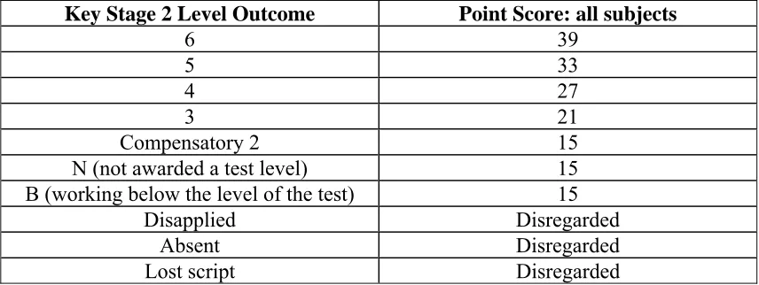
A further approach to the assessment of value added is that published in the DfES Secondary School Performance Tables 2002 (DfES, 2003a), following the DfES’s Pilot Value Added Study. This calculates value-added measures between KS2 and KS3, and between KS3 and GCSE/GNVQ, according to the following method. For the KS2 to KS3 measure of value added, the data used are those for pupils who were eligible for KS3 assessment in 2002 and on the school roll at the time of the KS3 assessment in 2002, and for whom matching KS2 prior attainment data was available. The value-added calculations exclude all pupils for whom results are disregarded at KS2 or KS3 according to Tables 6.1 and 6.2 below, with the exception that an input score of zero is used if the pupil was disapplied in all three subjects or had a combination of disregarded and disapplied results at KS2 and achieved at least one KS3 result at levels 2-7. The input and output measures that were used for each pupil in the value-added calculation were the numerical averages of the point scores which the pupil achieved in the English, Maths and Science results at KS2 for the input measure and KS3 for the output measure (or where any result is disregarded, the average of the remaining non-disregarded point scores at that Key Stage).

Key Stage 2 Level Outcome Point Score: all subjects

6 39 5 33 4 27 3 21

Compensatory 2 15

N (not awarded a test level) 15

B (working below the level of the test) 15

Disapplied Disregarded Absent Disregarded

Lost script Disregarded

Source: DfES, 2003a

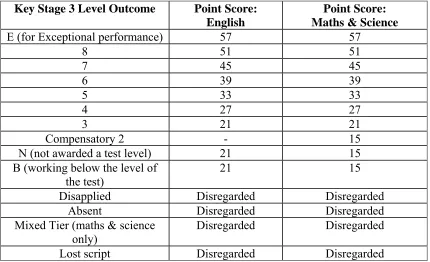
Key Stage 3 Level Outcome Point Score: English

Point Score: Maths & Science

E (for Exceptional performance) 57 57

8 51 51

7 45 45

6 39 39

5 33 33

4 27 27

3 21 21

Compensatory 2 - 15

N (not awarded a test level) 21 15

B (working below the level of the test)

21 15

Disapplied Disregarded Disregarded

Absent Disregarded Disregarded

Mixed Tier (maths & science only)

Disregarded Disregarded

Lost script Disregarded Disregarded

Source: DfES, 2003a

TABLE 6.2

The value-added score of a pupil is then calculated by comparing the pupil’s actual KS3 output

measure with the median level of the KS3 output measure across the whole country of pupils

in mainstream secondary schools with the same or similar input measure at KS2 to this pupil (with parallel separate calculations made for pupils in special schools). Table 6.3 below shows the median levels of the KS3 average point score output measure in mainstream secondary schools corresponding to different KS2 average point scores. Unlike multivariate regression analysis, where regression parameters would be used to predict the KS3 comparator for

different average point scores at KS2, the approach here is the non-parametric one of

selecting the corresponding national median level of performance at KS3 for each

KS2 Average Point Score KS3 National Median Average Point Score

0 21

15 21

17-18 21

19 23

21 27

23-24 29

25 31

27 35

29-30 37

31 39

33+ 43

Source: DfES, 2003a

TABLE 6.3

The corresponding median curve of the KS3 pupil-level National Median Average Point

Score (NMAPS) against the KS2 Average Point Score is not a straight line, being in particular flat at a value of 21, such as that achieved by a Level 3 outcome at KS3, for KS2 Average Point Scores between 0 and 18. The value-added score of a school between KS2 and KS3 is calculated as 100 plus the arithmetic mean of the value-added scores of all the pupils in the school for whom the value-added scores are calculated, rounded to one decimal point.

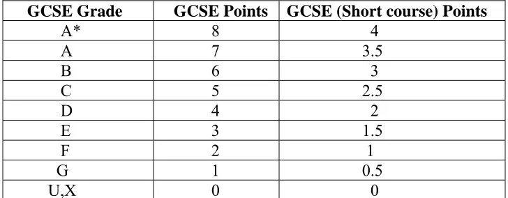
A similar approach has been used to calculate value-added scores between KS3 and GCSE/GNVQ. The point scores at GCSE is derived from the GCSE grade according to Table 6.4, with an equivalence table used to calculate corresponding point scores from GNVQs. Each

pupil’s GCSE/GNVQ output measure is calculated by summing their best 8 GCSE/GNVQ

point scores, and disregarding any other of their less good GCSE/GNVQ scores.

GCSE Grade GCSE Points GCSE (Short course) Points

A* 8 4

A 7 3.5

B 6 3

C 5 2.5

D 4 2

E 3 1.5

F 2 1

G 1 0.5

U,X 0 0

Source: DfES, 2003a

The input measure at KS3 for each pupil whose KS3 record can be matched with a corresponding GCSE/GNVQ score is calculated as the numerical average of their KS3 point score achieved in the English, mathematics and science tests, and the output measure. Their

value-added score between KS3 and GCSE/GNVQ is the difference between their

GCSE/GNVQ output measure and the national median level of the GCSE/GNVQ output

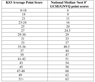
measure of all pupils with the same or similar input measures at KS3. The national median ‘best 8’ GCSE/GNVQ output scores for pupils in mainstream schools are shown in Table 6.5 below. Each school’s value added is again 100 plus the arithmetic mean of the value-added measures that have been calculated for pupils in the school, rounded to the nearest decimal point.

KS3 Average Point Score National Median ‘best 8’ GCSE/GNVQ point scores

0-18 6

19 9

21 11

23-24 16

25 20

27 24.5

29-30 29

31 33

33 37

35-36 40.5

37 44

39 47

41-42 51

43 54

45 58

47-48 60

49 62

51+ 63

Source: DfES, 2003a

TABLE 6.5

It should be noted that the above national median output levels are taken across all pupils,

both girls and boys, and irrespective of the proportion of pupils eligible for Free School Meals (FSM) or other variables related to the characteristics of the pupil intake.

However, several studies by the DfES (2001, 2002, 2003b) show that such additional

variables may well be relevant to the statistical explanation of the wide variations that exist

at the previous Key Stage. DfES (2003b) finds that at GCSE girls make more progress than

boys for each KS3 level of prior attainment, with a difference of 15 percentage points in 2002 in the percentage of pupils attaining 5 or more A*-C grades at GCSE for pupils with a level 5 at KS3, and with girls making more progress in English than boys at all Key Stages. Similar

significant differences in rates of pupil progress by gender were found in the earlier DfES

(2001) study based upon end-of-Key-Stage assessments in 2000.

The DfES (2003b) study also finds that non-FSM pupils make more progress from each prior

attainment level in each subject at every Key Stage than do FSM pupils. Moreover, while

pupils for whom English is an additional language (EAL) start below the national median

level, they in general make more progress than non-EAL pupils, tending to overcome some of their initial relative disadvantage as they become more proficient in English. Once they are performing above the national median level, they tend to make progress in line with non-EAL

pupils. Rates of progress also tend to vary with ethnicity. Amongst boys, Chinese pupils

progress most at all Key Stages, while amongst girls, Pakistani pupils start as one of the least progressing groups at KS2, but at GCSE are one of the best progressing groups. Black Caribbean pupils, whether boys or girls, or FSM or non-FSM pupils, are found to make below average progress at all Key Stages. White pupils are found to be one of the worst progressing ethnic groups at GCSE, and have the greatest difference (of 16 percentage points) between FSM and non-FSM pupils in progress to KS3 English and Science from the national median KS2 level.

School-level variables also appear to influence the rate of pupil progress. Non-FSM pupils are

Other school-type factors were found by DfES (2002) to make less difference than the

proportion of pupils eligible for FSM, and appear to account for only a small proportion of the wide spread of outcomes for pupils with similar prior attainments. Between KS2 and KS3, pupils in Voluntary Aided schools tended to make above average progress in English, while pupils in Foundation schools tended to make above average progress in mathematics, and pupils in Voluntary Controlled schools tended to make above average progress in science. Between KS3 and GCSE, pupils in Voluntary Aided schools and in Foundation Schools made above average progress, while those in Voluntary Controlled schools made below average progress in general. DfES (2002) also found that on average pupils in secondary faith schools made similar progress to pupils in all secondary maintained mainstream schools, except for slightly superior progress in KS3 English.

Between KS2 and KS3, in each core subject, pupils in specialist schools on average made

slightly more progress than pupils in all maintained mainstream schools. During KS4 they

made 1 or 2 GCSE points more progress than pupils in all schools. Pupils in Beacon Schools

made a fifth of a level more progress in English and a tenth of a level more progress in mathematics and science between KS2 and KS3 than pupils in all secondary maintained mainstream schools. At GCSE/GNVQ, pupils in Beacon Schools at the lower end of the prior attainment range made on average 4 GCSE points more progress than in all maintained mainstream schools, whereas at the upper end of the prior attainment range DfES (2002) found that they made on average 2 GCSE points difference. In mathematics and science, pupils in

schools in Education Action Zones (EAZs) were found to make similar progress between

KS2 and KS3 to pupils in all secondary maintained mainstream schools with broadly equivalent FSM proportions, whereas in KS3 English they made on average an eighth of a level less. Between KS3 and GCSE, pupils in EAZ schools also made similar progress to pupils in all secondary maintained mainstream schools with broadly equivalent FSM proportions, except that at the highest levels of prior attainment, pupils in EAZ schools made on average about 1 GCSE point more progress and those at the lowest levels of prior attainment, pupils in EAZ schools made on average about 1 GCSE point less progress. In addition for pupils in schools with FSM percentages in the range 21-35 per cent, EAZ schools made about 1 GCSE more progress.

Pupils in schools in Excellence in Cities (EiC) schools were found by DfES (2002) to make

broadly equivalent FSM proportions, with a difference that increased to about an eighth of a level at the highest levels of prior attainment. A similar difference at the upper levels of prior attainment was found in KS3 mathematics and science, but pupils with prior attainments of below an average level 5 in EiC schools made similar progress in KS3 mathematics and science. However, between KS3 and GCSE, pupils in EiC schools made about 1 GCSE point more progress for similar prior attainment levels than pupils in all secondary maintained mainstream schools with broadly equivalent FSM proportions, but with this difference increasing to about 2 GCSE points at the extreme ends of the prior attainment range.

Pupils in non-selective single sex schools were found to make on average more progress than

pupils of the same gender in non-selective mixed schools at both KS3 and KS4, particularly in

English. Between KS2 and KS3, pupils in designated selective LEAs who were at the upper end of the prior attainment range on average were found to make a quarter of a level more progress than pupils elsewhere, but similar progress in core subjects at the lower end of the prior attainment range. However, between KS3 and GCSE/GNVQ, pupils throughout the prior attainment range made about 1-2 GCSE points less progress in the designated selective LEAs

than elsewhere. School size also appears to have some impact on pupil progress. Pupils in

schools with year group cohorts of less than 100 pupils made less progress, even after adjusting for differences in FSM proportions. However, the size of the year group cohort appears not to affect the rate of pupil progress so long as it is greater than 100.

Rates of pupil progress may also vary over time. Between 2001 and 2002, DfES (2003b)

found that the rate of pupil progress at KS3 decreased in each subject measured in terms of the percentage of pupils attaining either KS3 level 5 or above, or level 6 or above, for every KS2 prior attainment level. The reason given for this is that the improvements made at KS2 between 1998 and 1999 have not fed through to similar improvements at KS3 from 2001 to 2002. Progress at KS3 has also decreased in English and mathematics for almost all KS2 prior attainment levels between 1999 and 2002. A decrease in the rate of pupil progress is also found between 2001 and 2002 of 3 and 2 percentage points in those gaining 5 or more GCSE A*-C grades for KS3 prior attainment levels 5 and 6 respectively, although progress has improved by 2 percentage points for KS3 prior attainment levels 4 and 5 between 1999 and 2002.

progress of individual pupils with similar levels of prior attainment. If this is so, there is a weaker case in assessing school effectiveness for computing school value-added measures, as in DfES (2003a), as the sum of the pupil-level differences between their actual performance at

a given Key Stage and the national median level of performance for the national cohort of

students with a similar level of prior attainment, irrespective of these other pupil- and

school-level variables. If these value-added measures are to be used as measures of school

effectiveness, or changes in school effectiveness following Academy status, there is a strong

case for taking into account those additional variables which have a significant systematic

influence on rates of pupil progress for the same level of prior attainment.

One, non-parametric, way of doing this would be by comparing each pupil’s actual level of performance at a given Key Stage with the median level of performance of those pupils

nationally with similar levels of prior attainment and similar levels of these other

statistically significant variables, including potentially those corresponding to gender, FSM

at pupil and school level, ethnicity, and school-type. However, if the number of such additional relevant variables is large, there may be a relatively small number of pupils in each relevant cell, with which to compare each pupil’s performance.

The above studies, moreover, do not provide any formal statistical tests of the significance of different pupil and school level variables in influencing the rates of pupil progress. In contrast

to multivariate regression analysis or multilevel modelling, the piecewise comparisons which

they involve, of the apparent influence of different variables on median levels of pupil progress, are less well suited to the identification of the relative strength and significance of each of several different pupil and school level variables which may be acting simultaneously on the rate of pupil progress in different subjects. It should also be noted that the KS3 and GCSE/GNVQ point scores used in the above analyses were based upon the levels that pupils

achieved in their Key Stage assessments and progress in discrete steps. Pupils who achieved

level 4, for example, received 27 points, and those who attained level 5 received 33 points. Small changes in the underlying distribution of pupil marks can then result in apparently large,

and seemingly significant, changes in average point scores and the associated median values

performance at either end of the range than the mean value, in circumstances where arguably

both high and low levels of educational performance should be fully taken into account in

assessing the overall impact of different variables.

Although the above non-parametric studies avoid explicit modelling of the multivariate

influences of the different variables on pupil progress, the problem of endogeneity bias does

not disappear as a result of a lack of such explicit modelling. As we note below, one important possible source of endogeneity bias is the existence of a correlation between pupil prior attainment at KS3 and the school-level disturbance term that may reflect school effectiveness not only at GCSE but also at KS3. Studies of value added from KS3 to GCSE that draw heavily on data where KS3 and GCSE examinations are both taken within the same school may then be particularly subject to such endogeneity bias.

Since pupil progress may indeed depend upon additional pupil- and school-level variables, a more explicit multivariate parametric estimation procedure has more recently been pursued by

the DfES as part of its Contextual Value Added (CVA) project. This is discussed more fully

7. AGGREGATION ISSUES

The desirability of disaggregating data to the lowest level at which the variables are likely to

have their impact is emphasised by the misleadingly high correlations which can occur between aggregated data at a higher level of analysis. As our earlier discussion of the ‘ecological fallacy’ emphasised, regression analyses of school-level mean values of

educational performance on school-level mean variables, such as school context variables, may yield biased estimates both of the regression coefficients and the variance explained, compared to disaggregated estimates based upon pupil-level data (see also Woodhouse and Goldstein,

1988; Woodhouse, 1990; Fitz-Gibbon, 1996). The problem of aggregation bias when the

coefficients in individual micro-relationships differ across individuals was emphasised by Theil (1954). While Zeller (1966) showed that in a random coefficient model an OLS estimate of the aggregate relationship can provide an unbiased es