A Statistical Tree Annotator and Its Applications

Proceedings of the 49th Annual Meeting of the Association for Computational Linguistics, pages 1230–1238,

A Statistical Tree Annotator and Its Applications

Xiaoqiang Luo and Bing Zhao

IBM T.J. Watson Research Center 1101 Kitchawan Road Yorktown Heights, NY 10598

{xiaoluo,zhaob}@us.ibm.com

Abstract

In many natural language applications, there is a need to enrich syntactical parse trees. We present a statistical tree annotator augmenting nodes with additional information. The anno-tator is generic and can be applied to a va-riety of applications. We report 3 such ap-plications in this paper: predicting function tags; predicting null elements; and predicting whether a tree constituent is projectable in ma-chine translation. Our function tag prediction system outperforms significantly published re-sults.

1 Introduction

Syntactic parsing has made tremendous progress in the past 2 decades (Magerman, 1994; Ratnaparkhi, 1997; Collins, 1997; Charniak, 2000; Klein and Manning, 2003; Carreras et al., 2008), and accu-rate syntactic parsing is often assumed when devel-oping other natural language applications. On the other hand, there are plenty of language applications where basic syntactic information is insufficient. For instance, in question answering, it is highly desir-able to have the semantic information of a syntactic constituent, e.g., a noun-phrase (NP) is a person or an organization; an adverbial phrase is locative or temporal. As syntactic information has been widely used in machine translation systems (Yamada and Knight, 2001; Xiong et al., 2010; Shen et al., 2008; Chiang, 2010; Shen et al., 2010), an interesting question is to predict whether or not a syntactic con-stituent is projectable1 across a language pair.

1

A constituent in the source language is projectable if it can be aligned to a contiguous span in the target language.

Such problems can be abstracted as adding addi-tional annotations to an existing tree structure. For example, the English Penn treebank (Marcus et al., 1993) contains function tags and many carry seman-tic information. To add semanseman-tic information to the basic syntactic trees, a logical step is to predict these function tags after syntactic parsing. For the prob-lem of predicting projectable syntactic constituent, one can use a sentence alignment tool and syntac-tic trees on source sentences to create training data by annotating a tree node as projectable or not. A generic tree annotator can also open the door of solv-ing other natural language problems so long as the problem can be cast as annotating tree nodes. As one such example, we will present how to predict empty elements for the Chinese language.

has significant lower error rate than (Blaheta and Charniak, 2000; Lintean and Rus, 2007a).

The rest of the paper is organized as follows. Sec-tion 2 describes our tree annotator, which is a con-ditional log-linear model. Section 3 describes the features used in our system. Next, three applications of the proposed tree annotator are presented in Sec-tion 4: predicting English funcSec-tion tags, predicting Chinese empty elements and predicting Arabic pro-jectable constituents. Section 5 compares our work with some related prior arts.

2 A MaxEnt Tree Annotator Model

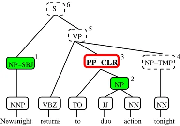
The input to the tree annotator is a tree T. While T can be of any type, we concentrate on the syntac-tic parse tree in this paper. The non-terminal nodes, N = {n : n ∈ T} of T are associated with an order by which they are visited so that they can be indexed asn₁,n₂,· · ·,n|T_|, where|T|is the num-ber of non-terminal nodes in T. As an example, Figure 1 shows a syntactic parse tree with the pre-fix order (i.e., the number at the up-right corner of each non-terminal node), where child nodes are vis-ited recursively from left to right before the parent node is visited. Thus, the NP-SBJnode is visited first, followed by the NP spanning duo action, followed by thePP-CLRnode etc.

With a prescribed tree visit order, our tree annota-tor model predicts a symbolli, where li takes value from a predefined finite setL, for each non-terminal nodeniin a sequential fashion:

P(l₁,· · ·, l_|T_||T) =

|T_|

Y

i₌₁

P(li|l₁,· · · , li−1, T) (1)

The visit order is important since it determines what are in the conditioning of Eq. (1).

P(li|l₁,· · · , li₋₁, T)in this work is a conditional log linear (or MaxEnt) model (Berger et al., 1996):

P(li|l₁,· · · , li−1, T)

= exp

P

kλkgk(l i₋₁

1 , T, li)

Z(l₁i−1, T) (2) where

Z(li₁−1, T) =X x_∈L

exp X k

λkgk(li₁−1, T, x)

3

VBZ TO JJ NN NN

Newsnight returns to duo action tonight NP

VP S

NP−TMP

2

4 5

6

NP−SBJ 1

PP−CLR

NNP

Figure 1: A sample tree: the number on the upright corner of each non-terminal node is the visit order.

is the normalizing factor to ensure that P(li|l₁,· · ·, li₋₁, T) in Equation (2) is a prob-ability and{gk(l₁i−1, T, li)}are feature functions.

There are efficient training algorithms to find op-timal weights relative to a labeled training data set once the feature functions {gk(l

i₋₁

1 , T, li)} are

se-lected (Berger et al., 1996; Goodman, 2002; Malouf, 2002). In our work, we use the SCGIS training al-gorithm (Goodman, 2002), and the features used in our systems are detailed in the next section.

Once a model is trained, at testing time it is ap-plied to input tree nodes by the same order. Figure 1 highlights the prediction of the function tag for node 3(i.e., PP-CLR-node in the thickened box) after 2 shaded nodes (NP-SBJnode andNPnode) are pre-dicted. Note that by this time the predicted values are available to the system, while unvisited nodes (nodes in dashed boxes in Figure 1) can not provide such information.

3 Features

The features used in our systems are tabulated in Ta-ble 1. Numbers in the first column are the feature in-dices. The second column contains a brief descrip-tion of each feature, and the third column contains the feature value when the feature at the same row is applied to thePP-node of Figure 1 for the task of predicting function tags.

Feature 9 and 10 are computed from past pre-dicted values. When predicting the function tag for thePP-node in Figure 1, there is no predicted value for its left-sibling and any of its child node. That’s why both feature values are NONE, a special sym-bol signifying that a node does not carry any func-tion tag. If we were to predict the funcfunc-tion tag for theVP-node, the value of Feature 9 would beSBJ, while Feature 10 will be instantiated twice with one value beingCLR, another beingTMP.

No. Description Value

1 current node label PP

2 parent node label VP

3 left-most child label/tag TO

4 right-most child label/tag NP

5 number of child nodes 2

6 CFG rule PP->TO NP

7 label/tag of left sibling VBZ

8 label/tag of right sibling NP

9 predicted value of left-sibling NONE

10 predicted value of child nodes NONE

11 left-most internal word to

12 right-most internal word action

13 left neighboring external word returns

14 right neighboring external word tonight

15 head word of current node to

16 head word of parent node returns

17 is current node the head child false 18 label/tag of head child TO

19 predicted value of the head child NONE

Table 1: Feature functions: the 2nd column contains the descriptions of each feature, and the 3rd column the fea-ture value when it is applied to thePP-node in Figure 1.

Feature 11 to 19 are lexical features or computed from head nodes. Feature 11 and 12 compute the node-internal boundary words, while Feature 13 and 14 compute the immediate node-external boundary words. Feature 15 to 19 rely on the head informa-tion. For instance, Feature 15 computes the head word of the current node, which is tofor the PP -node in Figure 1. Feature 16 computes the same for the parent node. Feature 17 tests if the current node is the head of its parent. Feature 18 and 19 compute the label or POS tag and the predicted value of the head child, respectively.

Besides the basic feature presented in Table 1, we also use conjunction features. For instance, applying the conjunction of Feature 1 and 18 to thePP-node

in Figure 1 would yield a feature instance that cap-tures the fact that the current node is aPPnode and its head child’s POS tag isTO.

4 Applications and Results

A wide variety of language problems can be treated as or cast into a tree annotating problem. In this section, we present three applications of the statisti-cal tree annotator. The first application is to predict function tags of an input syntactic parse tree; the sec-ond one is to predict Chinese empty elements; and the third one is to predict whether a syntactic con-stituent of a source sentence is projectable, meaning if the constituent will have a contiguous translation on the target language.

4.1 Predicting Function Tags

In the English Penn Treebank (Marcus et al., 1993) and more recent OntoNotes data (Hovy et al., 2006), some tree nodes are assigned a function tag, which is of one of the four types: grammatical, form/function, topicalization and miscellaneous. Ta-ble 2 contains a list of function tags used in the English Penn Treebank (Bies et al., 1995). The “Grammatical” row contains function tags marking the grammatical role of a constituent, e.g., DTVfor dative objects, LGSfor logical subjects etc. Many tags in the “Form/function” row carry semantic in-formation, e.g.,LOCis for locative expressions, and

TMPfor temporal expressions.

Type Function Tags

Grammatical (52.2%) DTV LGS PRD PUT SBJ VOC Form/function (36.2%) ADV BNF DIR

EXT LOC MNR NOM PRP TMP Topicalization (2.2%) TPC

Miscellaneous (9.4%) CLF CLR HLN TTL

Table 2: Four types of function tags and their relative frequency

4.1.1 Comparison with Prior Arts

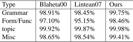
2-21 of Wall Street Journal (WSJ) data for training and Section 23 as the test set. We use all features in Table 1 and build four models, each of which pre-dicting one type of function tags. The results are tabulated in Table 3.

As can be seen, our system performs much better than both (Blaheta and Charniak, 2000) and (Lin-tean and Rus, 2007a). For two major categories, namely grammatical and form/function which ac-count for96.84%non-null function tags in the test set, our system achieves a relative error reduction of 77.1%(from (Blaheta and Charniak, 2000)’s1.09% to0.25%) and46.9%(from (Blaheta and Charniak, 2000)’s 2.90% to 1.54%) , respectively. The per-formance improvements result from a clean learn-ing framework and some new features we intro-duced: e.g., the node-external features, i.e., Feature 13 and 14 in Table 1, can capture long-range statis-tical dependencies in the conditional model (2) and are proved very useful (cf. Section 4.1.2). As far as we can tell, they are not used in previous work.

Type Blaheta00 Lintean07 Ours

Grammar 98.91% 98.45% 99.75%

Form/Func 97.10% 95.15% 98.46%

topic 99.92% 99.87% 99.98%

Misc 98.65% 98.54% 99.41%

Table 3: Function tag prediction accuracies on gold parse trees: breakdown by types of function tags. The 2nd umn is due to (Blaheta and Charniak, 2000) and 3rd col-umn due to (Lintean and Rus, 2007a). Our results on the 4th column compare favorably with theirs.

4.1.2 Relative Contributions of Features

Since the English WSJ data set contains newswire text, the most recent OntoNotes (Hovy et al., 2006) contains text from a more diversified genres such as broadcast news and broadcast conversation, we decide to test our system on this data set as well. WSJ Section 24 is used for development and Sec-tion 23 for test, and the rest is used as the training data. Note that some WSJ files were not included in the OntoNotes release and Section 23 in OntoNotes contains only 1640 sentences. The OntoNotes data statistics is tabulated in Table 4. Less than 2% of nodes with non-empty function tags were assigned multiple function tags. To simplify the system build-ing, we take the first tag in training and testing and

report the aggregated accuracy only in this section.

#-sents #-nodes #-funcNodes training 71,186 1,242,747 280,755

test 1,640 31,117 6,778

Table 4: Statistics of OntoNotes: #-sents – number of sentences; #-nodes – number of non-terminal nodes; #-funcNodes – number of nodes containing non-empty function tags.

We use this data set to test relative contributions of different feature groups by incrementally adding features into the system, and the results are reported in Table 5. The dummy baseline is predicting the most likely prior – the empty function tag, which indicates that there are 78.21% of nodes without a function tag. The next line reflects the performance of a system with non-lexical features only (Feature 1 to 8 in Table 1), and the result is fairly poor with an accuracy 91.51%. The past predictions (Feature 8 and 9) helps a bit by improving the accuracy to 92.04%. Node internal lexical features (Feature 11 and 12) are extremely useful: it added more than 3 points to the accuracy. So does the node external lex-ical features (Feature 13 and 14) which added an ad-ditional 1.52 points. Features computed from head words (Feature 15 to 19) carry information comple-mentary to the lexical features and it helps quite a bit by improving the accuracy by 0.64%. When all features are used, the system reached an accuracy of 97.34%.

From these results, we can conclude that, unlike syntactic parsing (Bikel, 2004), lexical information is extremely important for predicting and recover-ing function tags. This is not surprisrecover-ing since many function tags carry semantic information, and more often than not, the ambiguity can only be resolved by lexical information. E.g., whether aPPis locative or temporal PPis heavily influenced by the lexical choice of theNPargument.

4.2 Predicting Chinese Empty Elements

pro-Feature Set Accuracy

prior (guess NONE) 78.21% Non-lexical labels only 91.52% +past prediction 92.04% +node-internal lexical 95.17% +node-external lexical 96.70%

+head word 97.34%

Table 5: Effects of feature sets: the second row contains the baseline result when always predictingNONE; Row 3 through 8 contain results by incrementally adding feature sets.

cessing. Recently, Chung and Gildea (2010) has found it useful to recover empty elements in ma-chine translation.

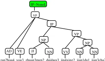
Since empty elements do not have any surface string representation, we tackle the problem by at-taching a pseudo function tag to an empty element’s lowest non-empty parent and then removing the sub-tree spanning it. Figure 2 contains an example tree before and after removing the empty element

*pro* and annotating the non-empty parent with

a pseudo function tag NoneL. The transformation procedure is summarized in Algorithm 1.

In particular, line 2 of Algorithm 1 find the lowest parent of an empty element that spans at least one non-trace word. In the example in Figure 2, it would find the topIP-node. Since*pro*is the left-most

child, line 4 of Algorithm 1 adds the pseudo function tagNoneLto the topIP-node. Line 9 then removes itsNPchild node and all lower children (i.e., shaded subtree in Figure 2(1)), resulting in the tree in Fig-ure 2(2).

Line 4 to 8 of Algorithm 1 indicate that there are 3 types of pseudo function tags: NoneL, NoneM, andNoneR, encoding a trace found in the left, mid-dle or right position of its lowest non-empty parent. It’s trivial to recover a trace’s position in a sentence fromNoneL, andNoneR, but it may be ambiguous forNoneM. The problem could be solved either us-ing heuristics to determine the position of a middle empty element, or encoding the positional informa-tion in the pseudo funcinforma-tion tag. Since here we just want to show that predicting empty elements can be cast as a tree annotation problem, we leave this op-tion to future research.

With this transform, the problem of predicting a trace is cast into predicting the corresponding

JJ

NN NN NN

NP NP

VP VP

(1) Original tree with a trace (the left−most child of the top IP−node) NP

NP

VP VP

NN NN NN

AD VE JJ _VV

IP IP−NoneL

ran2hou4 you3 zhuan3men2 dui4wu3 jin4xing2 jian1du1 jian3cha2

(2) After removing trace and its parent node (shaded subtree in (1)) NP

NONE AD

IP IP

VV VE

*pro* ran2hou4 you3 zhuan3men2 dui4wu3 jin4xing2 jian1du1 jian3cha2

Figure 2: Transform of traces in a Chinese parse tree by adding pseudo function tags.

Algorithm 1 Procedure to remove empty elements

and add pseudo function tags.

Input: An input tree

Output: a tree after removing traces (and their

empty parents) and adding pseudo function tags to its lowest non-empty parent node

1:Foreach tracet

2: Find its lowest ancestor nodepspanning at least one non-trace word

3: iftisp’s left-most child 4: add pseudo tagNoneLtop 5: else iftisp’s right-most child 6: add pseudo tagNoneRtop 7: else

8: add pseudo tagNoneMtop

pseudo function tag and the statistical tree annota-tor can thus be used to solve this problem.

4.2.1 Results

We use Chinese Treebank v6.0 (Xue et al., 2005) and the broadcast conversation data from CTB v7.02. The data set is partitioned into training, de-velopment and blind test as shown in Table 6. The partition is created so that different genres are well represented in different subsets. The training, de-velopment and test set have 32925, 3297 and 3033 sentences, respectively.

Subset File IDs

Training

0001-0325, 0400-0454, 0600-0840 0500-0542, 2000-3000, 0590-0596 1001-1120, cctv,cnn,msnbc, phoenix 00-06

Dev 0841-0885, 0543-0548, 3001-3075 1121-1135, phoenix 07-09

Test 0900-0931,0549-0554, 3076-3145 1136-1151, phoenix 10-11

Table 6: Data partition for CTB6 and CTB 7’s broadcast conversation portion

We then apply Algorithm 1 to transform trees and predict pseudo function tags. Out of 1,100,506 non-terminal nodes in the training data, 80,212 of them contain pseudo function tags. There are 94 nodes containing 2 pseudo function tags. The vast major-ity of pseudo tags – more then 99.7% – are attached to eitherIP,CP, orVP: 50971, 20113, 8900, respec-tively.

We used all features in Table 1 and achieved an accuracy of 99.70% on the development data, and 99.71%on the test data on gold trees.

To understand why the accuracies are so high, we look into the 5 most frequent labels carrying pseudo tags in the development set, and tabulate their per-formance in Table 7. The 2nd column contains the number of nodes in the reference; the 3rd column the number of nodes of system output; the 4th column the number of nodes with correct prediction; and the 5th column F-measure for each label.

From Table 7, it is clear that CP-NoneL and

IP-NoneL are easy to predict. This is not sur-prising, given that the Chinese language lacks of

2

Many files are missing in LDC’s early 2010 release of CTB 7.0, but broadcast conversation portion is new and is used in our system.

Label numRef numSys numCorr F1

CP-NoneL 1723 1724 1715 0.995 IP-NoneL 3874 3875 3844 0.992 VP-NoneR 660 633 597 0.923 IP-NoneM 440 432 408 0.936 VP-NoneL 135 107 105 0.868

Table 7: 5 most frequent labels carrying pseudo tags and their performances

complementizers for subordinate clauses. In other words, left-most empty elements under CP are al-most unambiguous: if aCPnode has an immediate

IPchild, it almost always has a left-most empty el-ement; similarly, if an IP node has a VPnode as the left-most child (i.e., without a subject), it almost always should have a left empty element (e.g., mark-ing the dropped pro). Another way to interpret these results is as follows: when developing the Chinese treebank, there is really no point to annotate left-most traces forCPand IPwhen tree structures are available.

On the other hand, predicting the left-most empty elements for VP is a lot harder: the F-measure is only 86.8% for VP-NoneL. Predicting the right-most empty elements under VP and middle empty elements underIPis somewhat easier: VP-NoneR

andIP-NoneM’s F-measures are 92.3% and 93.6%, respectively.

4.3 Predicting Projectable Constituents

The third application is predicting projectable con-stituents for machine translation. State-of-the-art machine translation systems (Yamada and Knight, 2001; Xiong et al., 2010; Shen et al., 2008; Chi-ang, 2010; Shen et al., 2010) rely heavily on syn-tactic analysis. Projectable structures are impor-tant in that it is assumed in CFG-style translation rules that a source span can be translated contigu-ously. Clearly, not all source constituents can be translated this way, but if we can predict whether a non-terminal source node is projectable, we can avoid translation errors by bypassing or discourag-ing the derivation paths relydiscourag-ing on non-projectable constituents, or using phrase-based approaches for non-projectable constituents.

pro-NOUN

b# sbb " _" l# Alms&wl

the Iraqi official ’s sudden obligations

.

AltzAmAt

PREP

Because of "

NOUN

S

PP#

NP#1

NP#2

NP

PP

NP

AlErAqy .

PUNC PREP DET+NOUN DET+ADJ

ADJ PUNC

PUNC

Figure 3: An example to show how a source tree is annotated with its alignment with the target sentence.

jectable or non-projectable. The binary annotations can again be treated as pseudo function tags and the proposed tree annotator can be readily applied to this problem.

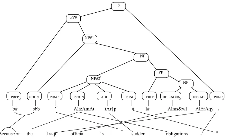
As an example, the top half of Figure 3 con-tains an Arabic sentence with its parse tree; the bot-tom is its English translation with the human word-alignment. There are three non-projectable con-stituents marked with “#”: the top PP# spanning the whole sentence except the final stop, andNP#1

and NP#2. The PP# node is not projectable due to an inserted stop from outside; NP#1is not pro-jectable because it is involved in a 2-to-2 alignment with the token b#outside NP#1; NP#2is aligned to a spanthe Iraqi official ’s sudden

obligations ., in which Iraqi official

breaks the contiguity of the translation. It is clear that a CFG-like grammar will not be able to gener-ate the translation forNP#2.

The LDC’s Arabic-English bilingual treebank does not mark if a source node is projectable or not, but the information can be computed from word alignment. In our experiments, we processed 16,125 sentence pairs with human source trees for training, and 1,151 sentence pairs for testing. The statistics of the training and test data can be found in Table 8, where the number of sentences, the number of non-terminal nodes and the number of non-projectable

nodes are listed in Column 2 through 4, respectively.

Data Set #Sents #nodes #NonProj

Training 16,125 558,365 121,201

Test 1,151 40,674 8,671

Table 8: Statistics of the data for predicting projectable constituents

We get a 94.6% accuracy for predicting pro-jectable constituents on the gold trees, and an 84.7% F-measure on the machine-generated parse trees. This component has been integrated into our ma-chine translation system (Zhao et al., 2011).

5 Related Work

ac-curacies for 4 types of function tags, and our results in Table 3 compare favorably with those in (Blaheta and Charniak, 2000). Lintean and Rus (2007a; Lin-tean and Rus (2007b) also studied the function tag-ging problem and applied naive Bayes and decision tree to it. Their accuracy results are worse than (Blaheta and Charniak, 2000). Neither (Blaheta and Charniak, 2000) nor (Lintean and Rus, 2007a; Lin-tean and Rus, 2007b) reported the relative usefulness of different features, while we found that the lexical features are extremely useful.

Campbell (2004) and Schmid (2006) studied the problem of predicting and recovering empty cate-gories, but they used very different approaches: in (Campbell, 2004), a rule-based approach is used while (Schmid, 2006) used a non-lexical PCFG sim-ilar to (Klein and Manning, 2003). Chung and Gildea (2010) studied the effects of empty cate-gories on machine translation and they found that even with noisy machine predictions, empty cate-gories still helped machine translation. In this paper, we showed that empty categories can be encoded as pseudo function tags and thus predicting and recov-ering empty categories can be cast as a tree anno-tating problem. Our results also shed light on some empty categories can almost be determined unam-biguously, given a gold tree structure, which sug-gests that these empty elements do not need to be annotated.

Gabbard et al. (2006) modified Collins’ parser to output function tags. Since their results for predict-ing function tags are on system parses, they are not comparable with ours. (Gabbard et al., 2006) also contains a second stage employing multiple clas-sifiers to recover empty categories and resolve co-indexations between an empty element and its an-tecedent.

As for predicting projectable constituent, it is re-lated to the work described in (Xiong et al., 2010), where they were predicting translation boundaries. A major difference is that (Xiong et al., 2010) de-fines projectable spans on a left-branching deriva-tion tree solely for their phrase decoder and models, while translation boundaries in our work are defined from source parse trees. Our work uses more re-sources, but the prediction accuracy is higher (mod-ulated on a different test data): we get a F-measure 84.7%, in contrast with (Xiong et al., 2010)’s 71%.

6 Conclusions and Future Work

We proposed a generic statistical tree annotator in the paper. We have shown that a variety of natural language problems can be tackled with the proposed tree annotator, from predicting function tags, pre-dicting empty categories, to prepre-dicting projectable syntactic constituents for machine translation. Our results of predicting function tags compare favor-ably with published results on the same data set, pos-sibly due to new features employed in the system. We showed that empty categories can be represented as pseudo function tags, and thus predicting empty categories can be solved with the proposed tree an-notator. The same technique can be used to predict projectable syntactic constituents for machine trans-lation.

There are several directions to expand the work described in this paper. First, the results for predict-ing function tags and Chinese empty elements were obtained on human-annotated trees and it would be interesting to do it on parse trees generated by sys-tem. Second, predicting projectable constituents is for improving machine translation and we are inte-grating the component into a syntax-based machine translation system.

Acknowledgments

This work was partially supported by the Defense Advanced Research Projects Agency under contract No. HR0011-08-C-0110. The views and findings contained in this material are those of the authors and do not necessarily reflect the position or policy of the U.S. government and no official endorsement should be inferred.

We are also grateful to three anonymous reviewers for their suggestions and comments for improving the paper.

References

Adam L. Berger, Stephen A. Della Pietra, and Vincent J. Della Pietra. 1996. A maximum entropy approach to natural language processing. Computational

Lin-guistics, 22(1):39–71, March.

and Dekai Wu, editors, Proceedings of EMNLP 2004, pages 182–189, Barcelona, Spain, July. Association for Computational Linguistics.

Don Blaheta and Eugene Charniak. 2000. Assigning function tags to parsed text. In Proceedings of the 1st

Meeting of the North American Chapter of the Associ-ation for ComputAssoci-ational Linguistics, pages 234–240.

Don Blaheta. 2003. Function Tagging. Ph.D. thesis, Brown University.

Richard Campbell. 2004. Using linguistic principles to recover empty categories. In Proceedings of the

42nd Meeting of the Association for Computational Linguistics (ACL’04), Main Volume, pages 645–652,

Barcelona, Spain, July.

Xavier Carreras, Michael Collins, and Terry Koo. 2008. TAG, dynamic programming, and the perceptron for efficient, feature-rich parsing. In Proceedings of

CoNLL.

E. Charniak. 2000. A maximum-entropy-inspired parser. In Proceedings of NAACL, Seattle.

David Chiang. 2010. Learning to translate with source and target syntax. In Proc. ACL, pages 1443–1452. Tagyoung Chung and Daniel Gildea. 2010. Effects of

empty categories on machine translation. In

Proceed-ings of the 2010 Conference on Empirical Methods in Natural Language Processing, pages 636–645,

Cam-bridge, MA, October. Association for Computational Linguistics.

Michael Collins. 1997. Three generative, lexicalised models for statistical parsing. In Proc. Annual

Meet-ing of ACL, pages 16–23.

Peter Dienes, P Eter Dienes, and Amit Dubey. 2003. An-tecedent recovery: Experiments with a trace tagger. In

In Proceedings of the Conference on Empirical Meth-ods in Natural Language Processing, pages 33–40.

Ryan Gabbard, Mitchell Marcus, and Seth Kulick. 2006. Fully parsing the Penn Treebank. In Proceedings of

Human Language Technology Conference of the North Amer- ican Chapter of the Association of Computa-tional Linguistics.

Joshua Goodman. 2002. Sequential conditional general-ized iterative scaling. In Pro. of the 40th ACL. Eduard Hovy, Mitchell Marcus, Martha Palmer, Lance

Ramshaw, and Ralph Weischedel. 2006. Ontonotes: The 90% solution. In Proceedings of the Human

Lan-guage Technology Conference of the NAACL, Com-panion Volume: Short Papers, pages 57–60, New York

City, USA, June. Association for Computational Lin-guistics.

Dan Klein and Christopher D. Manning. 2003. Accu-rate unlexicalized parsing. In Erhard Hinrichs and Dan Roth, editors, Proceedings of the 41st Annual

Meet-ing of the Association for Computational LMeet-inguistics,

pages 423–430.

Mihai Lintean and V. Rus. 2007a. Large scale exper-iments with function tagging. In Proceedings of the

International Conference on Knowledge Engineering,

pages 1–7.

Mihai Lintean and V. Rus. 2007b. Naive Bayes and deci-sion trees for function tagging. In Proceedings of the

International Conference of the FLAIRS-2007.

David M. Magerman. 1994. Natural Language Parsing

As Statistical Pattern Recognition. Ph.D. thesis,

Stan-ford University.

Robert Malouf. 2002. A comparison of algorithms for maximum entropy parameter estimation. In the Sixth

Conference on Natural Language Learning (CoNLL-2002), pages 49–55.

M. Marcus, B. Santorini, and M. Marcinkiewicz. 1993. Building a large annotated corpus of English: the Penn treebank. Computational Linguistics, 19(2):313–330. Adwait Ratnaparkhi. 1997. A Linear Observed Time

Statistical Parser Based on Maximum Entropy Mod-els. In Second Conference on Empirical Methods in

Natural Language Processing, pages 1 – 10.

Helmut Schmid. 2006. Trace prediction and recov-ery with unlexicalized PCFGs and slash features. In

Proceedings of the 21st International Conference on Computational Linguistics and 44th Annual Meet-ing of the Association for Computational LMeet-inguistics,

pages 177–184, Sydney, Australia, July. Association for Computational Linguistics.

Libin Shen, Jinxi Xu, and Ralph Weischedel. 2008. A new string-to-dependency machine translation algo-rithm with a target dependency language model. In

Proceedings of ACL.

Libin Shen, Bing Zhang, Spyros Matsoukas, Jinxi Xu, and Ralph Weischedel. 2010. Statistical machine translation with a factorized grammar. In Proceedings

of the 2010 Conference on Empirical Methods in Natu-ral Language Processing, pages 616–625, Cambridge,

MA, October. Association for Computational Linguis-tics.

Deyi Xiong, Min Zhang, and Haizhou Li. 2010. Learn-ing translation boundaries for phrase-based decodLearn-ing. In NAACL-HLT 2010.

Nianwen Xue, Fei Xia, Fu-Dong Chiou, and Martha Palmer. 2005. The Penn Chinese TreeBank: Phrase structure annotation of a large corpus. Natural

Lan-guage Engineering, 11(2):207–238.

Kenji Yamada and Kevin Knight. 2001. A syntax-based statistical translation model. In Proc. Annual Meeting

of the Association for Computational Linguistics.