Detection of Noncircularity and Eccentricity
of a Rolling Winder by Artificial Vision
Christophe Doignon
Laboratoire des Sciences de l’Image, de l’Informatique et de la T´el´ed´etection, UMR CNRS 7005, ´Equipe de Recherche Technologique en Enroulement-ERTno8, Boulevard S´ebastien Brant, 67400 Illkirch, France
Email: [email protected]
Dominique Knittel
Laboratoire des Sciences de l’Image, de l’Informatique et de la T´el´ed´etection, UMR CNRS 7005, ´Equipe de Recherche Technologique en Enroulement-ERTno8, Boulevard S´ebastien Brant, 67400 Illkirch, France
Email: [email protected]
Received 31 July 2001 and in revised form 13 March 2002
A common objective in the web transport industry is to increase the velocity as much as possible. Some disturbances drastically limit this velocity. Time-varying eccentricity of the rolling winder is one of the major disturbances which affect the quality of the rolling winder. This unsuitable factor can lead to a web break for a high-speed winding process. The main contribution of this work is to offer a new measurement technique that is able to provide on-line the estimation of the roll radius and its variations with a subpixel accuracy. A key feature within this work is the contour curvature classification by means of wavelets decomposition of the edge orientation function. We also propose a new model accounting for the increasing radius of the rolling winder, which confirms the experimental results and the reliability of the proposed approach.
Keywords and phrases:shape-preserved filtering, curvature analysis, wavelets decomposition, contours classification, ellipse fit-ting, pose from ellipse.
1. INTRODUCTION
Products made with paper, textile, metal, or polymers need to be winded and unwinded during an industrial process. A common objective is to increase as much as possible the web transport velocity while controlling tension of the web. How-ever, there exist many sources of disturbances like noncircu-larity of the roll, eccentricity of the roll, web sliding, tem-perature variations, variations in motor torque, . . . which are some limiting factors of performances. Since there exists a coupling introduced by elastic property of the web, distur-bances are transmitted to the web tension, resulting in a web break or fold. In an attempt to reduce these harmful effects, recent works on modelization and control for web handling applications are promising and can be found, for example, in [1, 2, 3]. They are mainly based on PID,H∞robust control,
fuzzy logic, or neural network approaches [4]: due to a wide-range variation of the roll radius, system dynamics consid-erably change (inertia is proportional to the fourth power of the roll radius). Few works in the image processing or com-puter vision fields applied to winding systems have been yet published. However, the use of a visual sensor through digital image analysis for supervising the quality of the roll is being emerging [5, 6]. Figure 2 shows two reels with equal length
but winded under different conditions: the speed and tension of the web were constant for the left reel while a too strong and variant tension and speed magnitude were applied on the web for the right reel.
Figure1: The experimental winding equipment.
Figure2: High quality (left) and low quality (right) of the resulted reel.
2. IMAGES SEQUENCE ANALYSIS
A fundamental requirement in vision systems is the abil-ity to extract from digital images primitives relevant to the observed scene. Edge contour segmentation and curve parametrization are therefore important stages for represent-ing boundary information in a structural form. Since we deal with grey level images, some classical preprocessings like contrasts enhancement by histogram equalization and non-linear median filtering (suppression of peak noise) are per-formed but are not described here.
2.1. Contours detection
Since we are concerned by the analysis of visual motion in a time-varying image sequence, we are interested in selecting pixels that significantly contribute to the motion field. The partial temporal derivative(ptd-image)is computed on two consecutive frames (see Figure 4) in order to build a fast edge detector as follows:
• in an attempt to detect “pixels in motion,” the absolute value of image subtraction is computed and applied to consecutive frames (theptd-image),
• locations of pixels (for which absolute difference in the
ptd-imageare greater than a threshold) are stored in a list. Detection of edges is performed with a directional filter in the original grey level image only for pix-els having corresponding location in the list and also for its eight-connected neighboring pixels. We choose the Canny filter as a directional gradient filter since it
provides the edge orientation. To make the implemen-tation as efficient as possible, we use the separability property of the Canny filter (this filter is often approx-imated with the first derivative of a continuous Gaus-sian functiong(x, y)), discrete kernels components are scaled and approximated by integers and lookup tables are also used to store the gradient magnitude entries. Furthermore, we fixed the standard deviation parame-ter according to Canny’s criparame-teria (good detection, good localization, and unicity of response) in order to con-sider always a unique set of masks. It is clear that this is a frequency limitation since this fix the width of grey-level transitions. With a standard deviation value of 1.5 for the Canny filter parameter, we select the fifteen most significant components of the two discrete con-volution kernels as an approximation of the continu-ous convolution kernels for the two operators∂g/∂x
and∂g/∂y (see Figure 5). This yields two (3×5 and 5×3) masks. By this way, consuming time (the compu-tational time is about 18 minutes (see Section 4 for de-tails about the platform)) is significantly reduced and static background of the observed scene is removed (see Figure 6).
Canny’s detector always yields edges with many pixels of thickness. Two thinning operations are performed on the extracted set of edges based on the comparison of gradient magnitude and orientation of each pixel with their neigh-bors within the edge (nonmaxima suppression) producing a 1-pixel wide edge: this is a requirement for the apply of the
contour following method[7] to edges tracking. Edges track-ing is the process of associattrack-ing nearby edge points so as to create a connected boundary. At any detected edge, this pro-cess selects, among the set of the 8-nearest neighbors, the next one to include in a list (and labeled or simply deleted in the gradient image) producing a displacement through this list. This process is significantly optimized if thinning oper-ations are previously done (this confers the ability to begin the search for the next edge with the direction of the previ-ous displacement).
Contours in the list are merged by using a process called
Figure3: Some images of the rolling winder during the sequence.
Figure4: Some substractions of two successive frames: irrelevant static background has been removed from these three ptd-images (a bina-rization has been carried out for a good print).
into a single contour. Contours that are too short for a fu-ture classification are rejected.
2.2. Gradient phase smoothing
The sequence of operations of most computer vision systems begins by detecting and locating some features in the input images. To achieve this, edge contours have to be expressed in a form suitable for classification. A global representation based on set of moments or Fourier descriptors is unsuit-able when partial objects or image features are involved, and it is not suited for object location. Local representation as edge orientation function (extracted from the gradient phase signal), and its derivatives, is more interesting since it is not strongly affected by partial occlusions and it allows to define differential invariants under scaling, translation, and rota-tion transformarota-tions. Furthermore, the edge detecrota-tion gives this information in a nearly continuous space as Canny filter contributes to gradient phase smoothing. In this representa-tion, local edge orientation is expressed as a one-dimensional function ofθ(s) wheresis the curvilinear abscissa. Disconti-nuities inθ(s) and its derivatives mark limits between ele-mentary fragments of a contour and reflect transitions be-tween them.
A major problem of methods relying on the orientation function and its derivatives is their sensitivity to noise. How-ever, application of classical filtering has harmful effects like attenuation of discontinuities, change of shape, blurring ef-fects, and so forth. This complicates the detection of singu-lar points. Consequences are more severe for smoothed por-tions of contours for which discontinuities related to singular
points only appear in the high-degree derivatives of the ori-entation function. A simple noise filtering procedure may lead to a delocalization, or even to a loss of these salient points. Wuesher and Boyer [9] smooth at first the curvature function (first derivative of the orientation) using a Gaussian kernel with a low smoothing parameter in order to reduce the blurring effect and to preserve valid high frequency shape information. However, in that way, the noise was not well attenuated and they were constrained to apply a nonlinear filter to reduce the remaining noise. The polygonal approx-imation of curves proposed by Pikaz and Dinstein [10] sig-nificantly reduces the noise but the implemented algorithm is complex and highly time-consuming. Our objective is to find a linear smoothing filter that is a trade-offbetween a maxi-mum reduction of noise and a good preservation of high fre-quency informations in the orientation (or gradient phase) function.
Weiss [11] defined what he called the power preserving filter as follows: considering the Taylor expansion f(x) =
(f(n)/n!)xnof a function f(x) representing the input sig-nal, a filter of orderlis a filter which preserves the powerxn up to orderlwith respect to the convolutionFl(x, σ)∗xn=
xn, (forn = 0, . . . , l) where F
l(x, σ) is the impulsional re-sponse of the filter. Weiss showed that moments of such fil-ters, defined by
mn=
w
−wx nF
(a) (b)
−5 −4 −3 −2 −1 0 1 2 3 4 5
0 0.05 0.1 0.15 0.2 0.25 0.3 0.35
(c)
−5 −4 −3 −2 −1 0 1 2 3 4 5
−0.15 −0.1 −0.05
0 0.05 0.1 0.15
(d)
Figure5: The first derivative of a Gaussian as an approximate solution of Canny’s criteria for edges detection (σ =1.5). (a) and (b) partial derivatives of the 2D Gaussian filter with respect toxandy, (c) the 1D Gaussian function, and (d) its first derivative.
(a) (b) (c)
Figure6: (a) Part of original image, (b) partial temporal derivative on consecutive frames, (c) gradient magnitude computed in the original image for motion pixels and their neighborhood.
x = x). Errors due to additive terms and causing blurring effect or bias are expressed by
ᏯWeiss=
ml+1
(l+ 1)!
σl+1
s0 .
(2)
The smaller (2), the best is the filter. σ is the smooth-ing parameter,lis the order of the filter, ands0 is a scale of the smoothed function. In our case, it can be taken as the
−300 −200 −100 0 100 200 300
Figure7: (a) Impulsional responses, (b) magnitude-frequency re-sponses, (c) phase-frequency responses for Butterworth (solid), Chebyshev (+), and elliptic (dashed) filters.
0 2 4 6 8 10 12 14 16 18 20
Figure8: The preserving shape criterionᏯWeisswith respect to the smoothingσparameter: Chebyshev (-·-·), elliptic filter (—), But-terworth filter (solid), Gaussian filter (....).
2.3. Classification
2.3.1 Multiscale detection of gradient phase discontinuities
(a) (b) (c)
Figure9: Curvature discontinuities detection. Fragment is defined between two discontinuities inside a contour. (a) a test image, (b) curva-ture discontinuities detection, (c) curvacurva-ture discontinuities found for the roll.
derivatives ([16, 17]). For a given scale, it takes a small value for the regular part of the signal and it explode at points where the signal or its derivatives undergo brutal changes. Then, wavelet transform can disclose both the discontinu-ities of the orientation function θ(s) and those of its first derivative (local curvature), second derivative (variations of the local curvature), and so forth. Considering the second-derivative of a Gaussian function (the Marr’s wavelet) as the prototype wavelet, this function vanishes quickly in both time and frequency spaces. Zero-crossings of the wavelet transform belong to a set of lines which converge at inflexion points of theθ(s) function for different scalesa. The choice of a continuous wavelet is more convenient than a dyadic wavelet for the study of the wavelet modulus along these lines [14].
The wavelet transformWf is defined as
Wf(a)=
as a prototype wavelet. (4)
Discontinuities detection gives as output a set of points which defines the ends of simple fragments composing a con-tour (see Figure 9). Concon-tour fragments are bounded by cur-vature discontinuities or by an endpoint and a discontinu-ity. In other words, there are as many contour fragments as curvature discontinuities detected minus one all along a con-tour. The wavelet transform modulus of these points is above a threshold. To improve their localization, we check neigh-borhoods afterwards. The aim of thresholding is to eliminate false discontinuities due to remaining noise in the orienta-tion funcorienta-tion after the linear smoothing operaorienta-tion. We have to estimate statistics of noise in the wavelet transform of the smoothed orientation function. We model the whole process by a succession of lowpass filters followed by the bandpass fil-ter corresponding to the wavelet transform. The varianceσ2 m
of the output noise can be computed if the input is the ori-entation functionθ(s) to which white noisen(0, σ2
n) is added [15]. We choose a threshold value greater than σm. In our experiments, a threshold value of 2.5σm has proven to be sufficient. Thus, we classified image contours between two discontinuities (or between an endpoint and a discontinu-ity) as follows: the wavelet transform of an orientation func-tion corresponding to a straight line fluctuates around zero, on the contrary it keeps a constant sign for a curve without inflexion point (like an elliptic arc for instance). Therefore, by counting the zero-crossings of the wavelet transform of orientation function we can know whether it corresponds to a straight line or not (see Figures 10 and 11).
2.3.2 Location of the outer contour
A list of contour fragments is built with fragments not corre-sponding to straight line. Some small fragments are rejected because they can be interpreted as the projections of lim-its between inner layers of the roll and an approximation of such portions of contours with a simple ellipse fitting is un-tractable (as a limit, these arcs look like a noisy line). How-ever, since all contour fragments contribute to the same cen-ter (but not the same radius), we derive an estimate for the localization of this center based on a modified circular fit-ting. To find that global centerC=(xc, yc)T, we can proceed in three stages through the list of contour fragments:
(1) For any pair of pixelsQi=(xi, yi)TandQj=(xj, yj)T of the same contour fragmentc, its contribution to a circular fitting is computed as
A simple difference on previous equations eliminates the radius parameter and provides a linear relation with respect to the center coordinates as unknown:
0 50 100 150 200 250 300 350 400
Figure10: (a) A contour of the roll, (b) the 1D corresponding cur-vature variations.
For a contour fragment withNcpixels,Nc−1 relations as above contribute for estimating the global center.
(2) Consider the next fragment (c+ 1) in the list of con-tour fragment and repeat the first stage until the end of the list is reached.
ple concatenation of all equations (6) obtained from all con-tour fragments. The Least Mean Square (LMS) solution gives an estimateC=(xc, yc) of that global center.
We point out that the right size of (6) may be very small. A data normalization is needed to avoid numerical instabil-ity of a homogeneous linear system. Furthermore, a judi-cious choice of the couple (Qi, Qj) can be simply obtained by browsing the list in both senses (j=Nc−i) or by shifting the index (j=Nc/2+i) . Finally, fragments are sorted accord-ing to the Euclidean distance (an average along the fragment)
from that center. Farthest fragments of contours have been kept and reassembled to approximate the outer profile of the roll with an ellipse fitting (see Figure 12).
3. ELLIPSE FITTING
Particularly, we have been interested in approximating con-tour fragment with elliptic features. This kind of geometric feature strongly constrains the 3D point of view. Thus, it is salient for object localization and orientation if it can be de-tected in a reliable manner. An ellipse can be represented with the quadratic algebraic equation
with the quadratic constraintb2−4ac <0. Ellipse parameters are components of the vectora=(a, b, c, d, e, f)T. There are many ellipse fitting methods available in the literature. Meth-ods based on Hough transform [18] are not suitable for our purpose as they are computationally too expensive. Classical least square method gives acceptable results for long arcs cov-ering a large portion of the ellipse with Gaussian noise other-wise estimation is biased. Extended Kalman filter avoids this drawback but the problem persists in the case of shallow arcs with high curvature ([15, 19]). Porril [20] suggested a bias-corrected Kalman filter based on the likelihood principle to overcome this problem. Since in (7) ellipse parameters have been defined up to a scale factor, all previous methods usually assume that f =1,a2+c2+b2/2=1,a+c=1, orE =1. It is clear that none of these constraints is adequate to segre-gate ellipse from other conics. Recently, Pilu [21] proposed a method based on the minimization of algebraic distance solved with the generalized eigenvalue problem. By using a prenormalization data processing (consisting in prescaling and translating coordinates (x, y)) and Cholesky decompo-sition, we propose to minimize the following criterion:
Figure11: Detection of nonlinear contour fragments of the roll.
Figure12: Extraction of outer contour fragments of rolling winder during the sequence.
Figure13: Ellipse fittings of outer contour fragments of the roll.
Figure14: Ellipse fittings superposed to grey level images.
Derivatives ofᏯwith respect to vectors a1 anda2 pro-vide an analytic solutiona for the smallest eigenvalueλ
1
This is the decomposition of the criterion used by Pilu but with a non-rank-deficient constraint matrixC. Thus, vectors
a1anda2can be expressed by
a2= −S−21ST12a1, (11)
Sa1=λCa1 (12) with the scatter matrixS
S=S1−S12S−21ST12, S1=X1TX1,
S2=X2TX2, S12=X1TX2.
(13)
The only valid solution corresponds to the single negative eigenvalueλof (12). The proposed method is a good trade-offbetween computational time and unbiased results in the presence of noisy data (mainly due to quantization and thin-ning operations) or outliers (one can see in Figures 12 and 13 that some inner layers are also selected).
4. POSE FROM ELLIPSE
Here, we remember the pose recovery from an ellipse (see [22]). The problem is, given a known ellipse on the world plane and its corresponding conic in the image, determine the pose of the world plane. The solution is in two stages:
(1) determine the orientationRceof the plane,
(2) determine the orthogonal distance d⊥ of the plane
from the camera origin.
The method exploits the property, unique to a conic that is an ellipse, that the back-projected curve must have the following representation:C0Xe2+A0Ye2=1 (A0>0 andC0>0) given in a canonical reference frame (principal axes reference frame
Re).
(1) Plane orientation
The conicEin the image is given by (7). We assume that the origin is at the principal point, and the distances are mea-sured in units of focal length. Then, the image curve defines a coneay2+bxy+cy2+d yz+exz+f z2=0 in 3D. The matrix in the quadratic form representation of this cone isxtEx=0 (wherex =(x, y, z)t) and may be diagonalized in the stan-dard manner by a 3D rotationR1of the coordinate system to eigenvector frame. We haveE=Rt1ER1andx=Rt1x, where (λ1 is then the only negative eigenvalue). Identification with coefficientsA0 and C0 is achieved by a second rota-tion about the y axis by an angle θ such that cosθ = ±(λ3−λ2(C0/A0))/(λ3−λ1), which sets both coefficients toλ2. There is therefore a four-fold ambiguity in the orienta-tion (θ, -θ,θ+π,π−θ). We haveE=Rt
The composite rotation from image plane to the plane that intersects the cone in an ellipse is thus x = Rt
cex, where
Rce = R1R2 and, consequently, the normal to the plane in the camera coordinate system isn = Rce(0,0,−1)t (the−1 accounts for the right-handed coordinate system).
(2) Plane distance
is the perpendicular distance of the plane from the origin. Fi-nally, the ellipse center is at the positiontce = Rce(α,0, d⊥)t
in the camera frame. To conclude this section, it is clear that values of C0 and A0 can be recovered if the orienta-tion Rce of the plane and the orthogonal distance d⊥ are
provided elsewhere, by a camera calibration procedure for instance.
5. RESULTS ANALYSIS
0 50 100 150 200 250 300 350 400 140
150 160 170 180 190
(a)
0 50 100 150 200 250 300 350 400
140 150 160 170 180 190 200 210 220 230 240
(b)
Figure15: (a) Minor/major semiaxes of the roll along the image sequence. (b) Experimental results of the mean roll radius and its model (in pixels).
0 50 100 150 200 250 300 350 400
280 290 300 310 320 330 340 350 360 370 380
Figure 16: Estimations of the roll center coordinates (in pixels) along the image sequence.
0 2 4 6 8 10
0 2 4 6
(a)
0 2 4 6 8 10 12
0 2 4 6 8 10 12
(b)
Figure 17: (a) Spectrogram of the sine-sliding behavior (from 8 to 6 Hz) of the motion of the roll center. (b) Temporal model of angular velocityΩ(t) (a=0.068, abscissa is unit time in second).
0 20 40 60 80 100 120 140 160
0 0.5 1 1.5 ×10⁻³
probe
h
h−
roll
ha
reference
control points
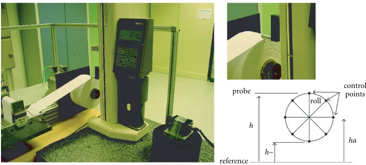
Figure19: The linear height measuring machine and locations of control points along the roll.
network) and developped under the C++/MPI programming language. Today, the whole image processing is achieved at a video rate of about 25 i/s. Figure 15 shows estimations of the minor and major semiaxes of the elliptic roll. As shown in Figure 15b, a mean value of the roll is computed for ev-ery image acquisition, compared with a model accounting for the radius increase and described below. This confirms the accuracy of the roll radius estimation in the image. The metric value of the roll radius can be found by means of a camera calibration [23] and the pose algorithm previously described. The computed mean square error of data points location from the estimated ellipse in Figure 18 is always less than√2.10−3≈1/20 pixel all along the sequence, so this con-firms our choice of an elliptical shape for the rolling winder profile.
In this paragraph, we modelize the increase of roll radius all along the sequence. It is of prime importance for an in-dustrial process control to predict its value. Denote byVand Ωthe linear and angular winding velocity, respectively, byr
the roll radius (the rolling winder is assumed to be circular in this paragraph), and byethe thickness of a web layer. Con-sidering that a small increase of the roll radius is proportional to a small increase of the angle, then
r(t)=r(0) + e 2π
t
0Ω(t)dt, (18)
V=r(t)Ω(t). (19) Assuming that the sliding effect is of low significance along the web, then the winding velocity is identical to the un-winding velocity. The consequence of such hypothesis is that
dV/dt=0 which leads to the simple differential equation
rd
2r
dt2 +
dr dt
2
= d
dt
rdr dt
=0. (20)
The solution for the radius is given by
r(t)=r(0)√1 +at, witha=eΩ(0)
πr(0) =
eV
πr2(0). (21)
From (19), the angular velocity can be also derived,Ω(t)=
Ω(0)/(1 +at). In spite of the fact that previous model has been built on pure kinematic considerations and with a rigid web, the course of the computed roll radius is very close to its estimates all along the sequence as shown in Figure 15b. Noise characteristics have been estimated to a value of 1.19 pixels for the standard deviation and 0.2 pixel for the mean.
Estimation of ellipse center coordinates are shown in Figure 16. Variations (typically of about 5 pixels) are due to the roll eccentricity. Frequency analysis was performed on thex-coordinate of the roll eccentricity. It relates a displace-ment of the main frequency mode and the angular velocity (see Figure 17). Although eccentricity is detected, noise is significant. A more accurate eccentricity detection could be achieved with more images per round (here, we typically have up to five images per round at 100 m/min).
In an attempt to validate the proposed method, we com-pare previous results for the roll radius estimates and its variations with those achieved straight with a high-accuracy height measuring machine. A Mitutoyo Linear Height LH600 has been installed on a marble surface. This machine pro-vides an elevation course of 600 mm and can be easily moved on the plate. It incorporates a reflective-type linear encoder which has a resolution down to 0.5µm. A 10 mm diameter ball probe is used for measuring the heighthwith respect to the surface plate (the reference). We also defined eight con-trol points per round by writing eight marks on the back side of the roll (see Figure 19). Since an accurate measure of the heighthaof roll axis is performed, the differenceh−ha pro-vides a measurement value for the roll radius at each con-trol point. We manually turned the roll of one eighth of a round to reach the next control point (exactly nine control points were used per round, the last one was identical to the first one up to a round). Since unwinding entirely the web in such a way is unpractical, we skip five rounds before begin-ning a new series of measurements. An image is grabbed by the camera for each series.
1 2 3 4 5 6 7 8 9 50
55 60 65
(a)
0 20 40 60 80 100 120 140 160 180 200 50
51 52 53 54 55 56 57 58 59 60
(b)
Figure20: (a) 180 measurements of the roll radius (in mm) with the LH600, (b) details of five series (45 measures) well arranged in the sequence of measures.
curve. Furthermore, it is clear that a significant noncircular-ity appears (see Figure 20b). To derive it, positions of control points all around the roll have been computed for each series in order to fit an ellipse.
Since an ellipse object (the roll) and its projection are both available, we can recover the orientation (only 2 de-grees of freedom since the roll is quite circular) and the po-sition of a reference object frame with respect to the camera frame provided that the camera calibration was previously done (the focal length value has been estimated in [23], and
f = 11.59 mm for the standard 12 mm optical lens used). In fact, since the calibration plane (coplanar patterns) has been placed just in front of the roll and since all calibration procedures using geometrical features simultaneously esti-mate intrinsic and extrinsic parameters (parameters of the Euclidean transformation), these values may be used to back-project the ellipse image to the 3D space. Results (in mm)
0 10 20 30 40 50 60 70 80 90 100
45 50 55 60 65
(a)
34 36 38 40 42 44 46
61.5 62 62.5 63 63.5 64 64.5 65 65.5 66
(b)
Figure21: Comparison between minor/major semiaxes measure-ments (in mm) on the static roll (dashed) and the back-projection to 3D space of minor/major semiaxes estimated from ellipse fitting (solid).
are shown in Figure 21 for the minor and major semiaxes (defined asC0 and
A0in Section 4) of the set of twenty ellipses. We observe in this figure that solid lines (estima-tions with the vision system) are closed to dashed lines (me-chanical measurements) with an absolute accuracy of about 0.4 mm for the minor semiaxis and 0.1 mm for the major semiaxis (the mean value of the roll radius has an accuracy better than 0.3 mm (|∆r/r| ≈0.5%)).
6. CONCLUSION
for the orientation function of edge contours is highly ef-ficient in comparison with the Gaussian filter. It trades off maximum elimination of noise with preservation of the high frequency information inside the gradient phase signal.
Another contribution of this work is the improve-ment of the Pilu’s technique for ellipse fitting. With a pre-normalization of data and the use of Cholesky decomposi-tion, an adequate criterion is proposed for analytically seg-regate ellipse from other conics. It is of most importance to take care of the fact that a common characteristic of methods based on the algebraic distance (the only methods providing analytical solutions for ellipse fitting with no approximation) is to be biased towards low-eccentricity for data covering a short arc of ellipse. That is why we focus on extracting data well-scattered along outer contours of the roll. We evaluate the validity of the proposed method by comparing the results obtained from the vision system to those measured with an accurate mechanical measuring machine. The roll radius has been well estimated with an accuracy (in 3D space) better than 0.3 mm, since noncircularity and eccentricity of the roll have been taken into account all through this work.
ACKNOWLEDGMENTS
The authors wish to thank the French Ministry of Research for financial support by means of the ERT-Project “High-speed handling and winding of flexible webs.”
REFERENCES
[1] K. N. Reid and K.-C. Lin, “Control of longitudinal tension in multi-span web transport systems during start-up,” inProc. 2nd International Conference on Web Handling, pp. 77–95, Ok-lahoma city, Okla, USA, 1993.
[2] H. Koc¸, D. Knittel, M. De Mathelin, and G. Abba, “Modeling and robust control of winding for elastic webs,” IEEE Trans-actions on Control System Technology, vol. 10, no. 2, 2002. [3] W. Wolfermann, “Compensation of disturbances in the web
force caused by a non-circular running winder,” inProc. In-ternational Conference on Web Handling, Oklahoma city, Okla, USA, 1999.
[4] S. Straub and D. Schr¨oder, “An example of an application of neural networks in rolling mills: compensation of the non-circularity of winders,” inIFAC Workshop on Motion Control, pp. 583–590, Munich, Germany, October 1995.
[5] B. Gueldenberg and Welp E. G., “Quantitative analysis of nip-induced tension by use of digital image processing,” in Proc. International Conference on Web Handling, Oklahoma city, Okla, USA, June 1999.
[6] C. Doignon and D. Knittel, “Non-circularity detection of a rolling winder by artificial vision,” inProc. 5th IEEE Inter-national Conference on Quality Control by Artificial Vision, Le Creusot, France, May 2001.
[7] C. Daul, Construction et utilisation de listes de primitives en vue d’une analyse dimensionnelle de pi`eces `a g´eom´etrie simple— Application `a la vision par ordinateur, Ph.D. thesis, Louis Pas-teur University, Strasbourg, France, January 1994.
[8] D. P. Huttenlocher and S. Ullman, “Recognizing solid objects by alignment with an image,” International Journal of Com-puter Vision, vol. 5, no. 2, pp. 195–212, 1990.
[9] D. M. Wuescher and K. L. Boyer, “Robust contour decompo-sition using a constant curvature criterion,” IEEE Trans. on
Pattern Analysis and Machine Intelligence, vol. 13, no. 1, pp. 41–51, 1991.
[10] A. Pikaz and I. Dinstein, “Using simple decomposition for smoothing and feature point detection of noisy digital curves,” IEEE Trans. on Pattern Analysis and Machine Intel-ligence, vol. 16, no. 8, pp. 808–813, 1994.
[11] I. Weiss, “High-order differentiation filters that work,” IEEE Trans. on Pattern Analysis and Machine Intelligence, vol. 16, no. 7, pp. 734–739, 1994.
[12] I. Weiss, “Noise-resistant invariants of curves,”IEEE Trans. on Pattern Analysis and Machine Intelligence, vol. 15, no. 9, pp. 943–948, 1993.
[13] V. Govindu and C. Shekhar, “Alignment using distributions of local geometric properties,”IEEE Trans. on Pattern Analysis and Machine Intelligence, vol. 21, no. 10, pp. 1031–1043, 1999. [14] J. Fayolle, L. Riou, and C. Ducottet, “Robustness of a multi-scale scheme of feature points detection,”Pattern Recognition, vol. 33, no. 9, pp. 1437–1453, 2000.
[15] N. Werghi and C. Doignon, “Contour decomposition with wavelet transform and parametrisation of elliptic curves with an unbiased extended Kalman filter,” inProc. 2nd Asian Con-ference on Computer Vision, vol. 3, pp. 186–190, Singapore, December 1995.
[16] S. G. Mallat, “A theory for multiresolution signal decompo-sition,” IEEE Trans. on Pattern Analysis and Machine Intelli-gence, vol. 11, no. 7, pp. 674–693, 1989.
[17] Y. Meyer,Les Ondelettes: Algorithmes et Applications, Armand Colin, Paris, 1992.
[18] C. C. Hsu and J. Huang, “Partitionned Hough transform for ellipsoid detection,” Pattern Recognition, vol. 23, no. 3, pp. 275–282, 1990.
[19] P. L. Rosin and G. A. W. West, “Segmenting curves into elliptic arcs and straight lines,” inProc. 3rd International Conf. on Computer Vision, pp. 75–78, Osaka, Japan, November 1990. [20] J. Porril, “Fitting ellipses and predicting confidence envelopes
using a bias corrected Kalman filter,” Image and Vision Com-puting, vol. 8, no. 1, pp. 37–41, 1990.
[21] M. Pilu, A. W. Fitzgibbon, and R. B. Fisher, “Ellipse-specific direct least-square fitting,” inProc. IEEE International Confer-ence on Image Processing, pp. 599–602, Lausanne, Switzerland, September 1996.
[22] M. Dhome, M. Richetin, J. T. Laprest´e, and G. Rives, “Spatial localization of modeled objects of revolution in monocular perspective vision,” inProc. 1st European Conference on Com-puter Vision, pp. 475–484, Antibes, France, April 1990. [23] C. Doignon and G. Abba, “A practical multi-plane method
for a low-cost calibration technique,” inProc. 5th European Control Conference, Karlsruhe, Germany, September 1999.
Christophe Doignonreceived the B.S. de-gree in Physics in 1987 and the Engineer-ing diploma in 1989 both from the ´Ecole Nationale Sup´erieure de Physique de Stras-bourg, France. He received the Ph.D. degree in computer vision and robotics from Louis Pasteur University, Strasbourg, France in 1994. In 1995 and 1996, he worked with the department of Electronics and Computer Science at University of Padua, Italy, for the
interests include modeling, identification, robust control, control of large scale