R E S E A R C H
Open Access
Schedule-based sequential localization in
asynchronous wireless networks
Dave Zachariah
1,2, Alessio De Angelis
1,3, Satyam Dwivedi
1*and Peter Händel
1Abstract
In this paper, we consider the schedule-based network localization concept, which does not require synchronization among nodes and does not involve communication overhead. The concept makes use of a common transmission sequence, which enables each node to perform self-localization and to localize the entire network, based on noisy propagation-time measurements. We formulate the schedule-based localization problem as an estimation problem in a Bayesian framework. This provides robustness with respect to uncertainty in such system parameters as anchor locations and timing devices. Moreover, we derive a sequential approximate maximuma posteriori(AMAP) estimator. The estimator is fully decentralized and copes with varying noise levels. By studying the fundamental constraints given by the considered measurement model, we provide a system design methodology which enables a scalable solution. Finally, we evaluate the performance of the proposed AMAP estimator by numerical simulations emulating an impulse-radio ultra-wideband (IR-UWB) wireless network.
Keywords: Wireless positioning; Cooperative localization; Asynchronous networks
1 Introduction
Localization of nodes in wireless networks is required in various applications [1]. In many scenarios, it is important for the nodes to know their own position and the position of other nodes in the network. As an example, the first responder situation considered in [2] benefits from self-localization and self-localization of other members by each member of the team.
Research done to address the above issues provides a variety of practical techniques. Extensive surveys of such techniques are provided in [3,4]. In time-of-arrival (TOA)-based systems, in particular, measuring time delays with the knowledge of anchor positions provides localization. The common challenges in location estima-tion are measurement noise, availability of accurate timing models and anchor uncertainty. Authors in [5-8] have proposed estimation methods and algorithms which are robust to anchor and timing uncertainty.
Cooperation between the nodes is used in position esti-mation solutions, as described in, e.g., [9-13]. Specifically, in [11], a distributed localization method is presented
*Correspondence: [email protected]
1ACCESS Linnaeus Centre, Signal Processing Lab, KTH Royal Institute of Technology, Stockholm, Sweden
Full list of author information is available at the end of the article
which is based on factor graphs and relies on cooperation and message-passing between nodes. The method enables accurate and robust localization in networks which are not fully connected and its performance is studied in a numer-ical simulation scenario based on experimental measure-ments. In [12], a cooperative localization algorithm is derived, which extends the non-parametric belief prop-agation (NBP) message-passing method first introduced in [13]. The method, which is based on approximating the junction-tree, improves performance with a reduced number of particles with respect to other NBP algorithms in the literature. The algorithm is validated by simulation and by applying it to experimental indoor ranging data acquired independently by [14].
The concept of schedule-based localization was intro-duced in [15-17]. It consists in the adoption of a common transmission sequence, known throughout the network. This concept achieves cooperative positioning in a decen-tralized manner even without communication overhead required for message passing [11-13]. Since the trans-missions are event-driven, the schedule-based localization concept provides other advantages, such as asynchronous operation and high update rate. The concept can be realized with low complexity hardware [18-21]. The
importance of removing communication overhead is par-ticularly high in systems like the tactical locator system, TOR, described in [22]. In the TOR system, the inter-agent ranging device is an ‘intelligent sensor’, among oth-ers, with an internal update rate which is high compared with the 1-Hz pace of the overall system. Such a system is employed in polluted RF environments where commu-nication resources have to be used for voice and video communication. Therefore, the use of schedule-based localization is motivated from a robust communication perspective, because it allows to replace all unnecessary communication/RF waveforms with predetermined inter-nal sequences to ensure maximum robustness.
In this paper, we provide a general Bayesian framework for schedule-based localization which takes into account uncertainty in anchor location and in timing devices. The contribution of this paper is the extension of previ-ous works in [15-17]. Here, we derive a new sequential estimator that, unlike previous works, is scalable to an arbitrary number of nodes and can be implemented online rather than processing large records of collected samples offline. The estimator also has an inherent robustness with respect to varying levels of measurement noise. In addition to this, we provide insight on the fundamen-tal constraints of the considered problem. Based on this analysis, we develop a methodology to obtain a scal-able solution, which achieves identifiability of individual nodes in a sequential manner. The methodology assists the formulation of the common transmission sequence.
Moreover, we evaluate the performance of the proposed estimator by numerical simulations in a case study con-sisting of a network of wireless nodes. For this scenario, numerous time-based localization technologies have been applied in the literature, including commercial communi-cation infrastructure, such as wireless local area networks [23] and personal area networks [24,25], as well as spe-cialized ranging and positioning systems such as chirp spread spectrum [26]. In this context, the impulse-radio ultra-wideband (IR-UWB) technology, cf. [27], is widely studied in the literature and has been considered for the implementation of cooperative localization methods in [11,28]. The sub-nanosecond time resolution property of IR-UWB, in fact, allows for centimeter-level measure-ment accuracy when applying time-of-arrival methods [29-31]. The characterization and modeling of the indoor UWB propagation channel are outside of the scope of the present paper and have been extensively studied in [32,33]. The method proposed in this paper is based on several assumptions that are valid in an IR-UWB set-up, which is our main interest. Therefore, here, we present numerical simulation results obtained using a network of IR-UWB nodes, where we set the parameters of the network configuration and error based on previous exper-imental work [18-21]. We highlight however that the
method is applicable for a plurality of other localization technologies,mutatis mutandis, yielding varying degrees of accuracy depending on the ability to resolve time sig-natures. Furthermore, we compare the performance of the proposed estimator to the fundamental limitations provided by a Cramér-Rao bound.
The remainder of this paper is organized as follows: Section 2 provides the problem formulation. Then, the sequential AMAP estimator is derived in section 3 along with a methodology for sequence construction. A numer-ical evaluation of the AMAP performance is provided in section 4. Finally, section 5 reports conclusions.
2 Problem formulation
We consider a fully connected wireless network ofN−1 transceiving nodes and an indefinite number of passive receiving nodes. The transceiving nodes transmit accord-ing to a given sequence, denotedT, which is known across the network. When a node transmits a signal, it is received by the other nodes, then the next node in the sequence transmits, making the process event-driven. Delays at all nodes are assumed to be analog as mentioned in [16-18]. On the basis of observed time intervals between received signals at an arbitrary node n, the goal is to achieve both self-localization and localization of other transceiv-ing nodes participattransceiv-ing in the sequence, T at node n
without the need for clock synchronization or additional communication.
Moreover, for the purposes of this paper, the passive receiving nodes are defined as non-transmitting nodes, which therefore do not take part in the transmission sequence. In this context, the goal of such nodes is self-localization and self-localization of the transceiving nodes.
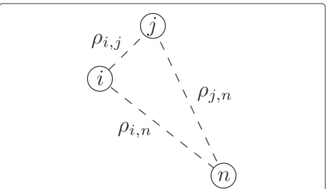
The signals are assumed to have a resolvable temporal signature that allows for timing events, e.g., pulses, symbol boundaries, etc. and the propagation velocitycis known. Let xi ∈ Rd denote the position of nodei, whered =
2 or 3, andρi,j xi−xj2 denote the range between
nodesiandj. Figure 1 illustrates the ranges between three different nodesi,j, andn.
Now suppose nodeiinitiates the transmission sequence and node j is the next node in the sequence. When it receives the signal, it transmits in return after a certain delayδj. The signal events at all nodes are then illustrated in Figure 2.
Using the relations to the ranges, the observed time interval at nodencan be expressed as [17,34,35]
y(i,j)= 1
cρi,j+δj+
1
cρj,n−
1
cρi,n+w
(i,j), (1)
Figure 1Example network setup involving the three nodesi,j, andn.
additive Gaussian noise model results in the least favor-able Cramér-Rao bound for parameter estimation. Under the model, therefore, any estimator that attains the lower bound can be considered min-max optimal [37].
If the next node in the sequence is denotedk, then the next observed time interval is
y(j,k)= 1
cρj,k+δk+
1
cρk,n−
1
cρj,n+w
(j,k), (2)
which uses one timing measurement from the previous observationy(i,j). Therefore, there is a correlation between all consecutive measurements. In addition to the random noise, the delayδjis subject to uncertainty due to hard-ware imperfections and is modeled as δj ∼ N(μδ,σδ2), whereμδis the nominal delay and the standard deviation σδis assumed to be known. To avoid signal collisions, it is necessary that the delays exceedρmax/c, whereρmaxis the
maximum range between any pair of transceivers and can easily be ensured in any bounded localization scenario.
Prior knowledge about the node positions in the net-work is modeled asxi ∼ N(μi,Ci), where the nominal
positionμiand error covariance matrixCi is set for alli
[5-7]. WithC−i 1 = 0we can also model complete igno-rance of a node position.
The goal is to formulate an estimator for any nodenthat performs self-localization as well as localization of an arbi-trary number of transceiving nodes, by processing batches of observed time intervals sequentially.
3 Proposed estimator
Letθ = [x1,· · ·,xN−1xN]∈ RdN denote the positions of all N − 1 transceiving nodes and the position of a passive receiver nodeN. Note that a necessary condition forxN to be identifiable is that localization is performed
at nodeN since, clearly, other nodes cannot localize the passive receiver nodes. For notational simplicity, letϑ
[θδ]∈ RT denote the sought parameters, where δ
contains the delays at theN −1 transceiving nodes and
T =dN+N−1.
We aim to formulate a sequential estimator that pro-cesses the observations in batches of B samples. The batches are indexed byb=1, 2,. . ., so that we can write
yb=hb(ϑ)+wb∈RB, (3)
where
hb(ϑ)=c−1Sbg(ϑ). (4)
The nonlinear mapping is g(ϑ) =[ρ(θ)δ], where
ρ(θ)contains theN(N−1)/2 unique rangesρi,jin a fixed
order. Here, the integer matrix Sb is determined by the
transmission sequence T for batchb, cf. (1). The noise followswb∼N(0,Rb)and
is an unknown band-diagonal matrix, as consecutive sam-ples are correlated.
In the next subsection, we derive an estimatorϑˆ which solves an approximate MAP problem using the obser-vation model in (3). Subsequently, in subsection 3.3, we provide a schedule construction approach to achieve parameter identifiability. In this subsection, we will also discuss how the sequential formulation of the estimation problem allows for robustness to random link failures in the network.
3.1 Approximate sequential MAP estimator
Suppose that, at batchb, we have a prior estimateϑˆb−1. We model the errors of ϑˆb−1 as zero-mean Gaussian with error covariance matrix Pb−1. For b = 1, ϑˆ0 =
[μ1,· · ·,μNμδ1]andP0=diag(C1,· · ·,CN,σδ2IN−1). The maximuma posterioriestimator ofϑandRbis given
by the maximization of
J(ϑ,Rb)lnp(yb|ϑ,Rb)+lnp(Rb)+lnp(ϑ)
where K is a constant. For tractability, we approximate
Rb σb2IB. Using a noninformative prior, we have
the approximate MAP estimator, denoted AMAP, can be written as
After solving (8), the estimate ϑˆb can be used for the next batchb+1. An approximate error covariance matrix
Pb can be derived using the information matrix b P−b1 0. Then using the approximation Rb σb2IB,
the information is additiveb = b−1+σb−2∂ϑhb∂ϑhb
[39]. Inserting the estimates, the latter term becomes ˆ
σb−2GbGb, whereGb=c−1Sb(ϑˆb)and(ϑ)∂ϑg(ϑ). Then we have the recursive update of the approximate error covariance matrix
To solve (8) iteratively, we linearizeg(ϑ) around an ini-tial estimate ϑˆ()b , i.e., g(ϑ) g(ϑˆ()b ) + ϑ˜, where
for notational simplicity. Then the cost function (9) is approximated by
The initial estimate is updated by the optimal increment ˆ
ϑ(b+1)= ˆϑ()b + ˜ϑ.
To compute the optimalϑ˜, we find a stationary point of
Vb()(ϑ˜)using the gradient
Note that whenBis small, the computational complexity of processing a batch is low as the computation ofϑˆbonly involves the nodes participating in the batchband there-foreGis a sparse matrix. Further, the matrix inversion on Line 12 in Algorithm 1 scales with the size of the batchB
rather than the total number of nodesN.
Algorithm 1 Sequential approximate MAP estimator
1: Input:yb,ϑˆb−1,Pb−1
2: Set:= −1,γb=B+2 andϑˆ 0 b= ˆϑb−1 3: repeat
4: :=+1
5: y˜b,=yb−c−1Sbg(ϑˆ
b)
6: G=c−1Sb(ϑˆ
b)
7: z= ˆϑb−1− ˆϑ
b
8: Repeat (13) until convergence
9: ϑˆb+1= ˜ϑ+ ˆϑb 10: until ˜ϑ2< ε
11: σˆb2= yb−c−1Sbg(ϑˆb)22/γb
12: Pb=Pb−1−Pb−1G
ˆ
σb2IB+GPb−1G −1
GPb−1 13: Output:ϑˆb,Pb
3.3 Sequence construction
To achieve identifiability, it is required that a subset of the transceiving nodes have highly informative priors. We denote such nodes as anchors. The other transceiving nodes are denoted as auxiliary nodes.
We propose a strategy to localize sequentially an arbi-trary number of auxiliary nodes at noden. First, we exploit the anchors to enable self-localization of node n. Sub-sequently, we devote each batch to the localization of one auxiliary node at a time. To achieve it, we interleave the transmissions of the auxiliary node with those of the anchors.
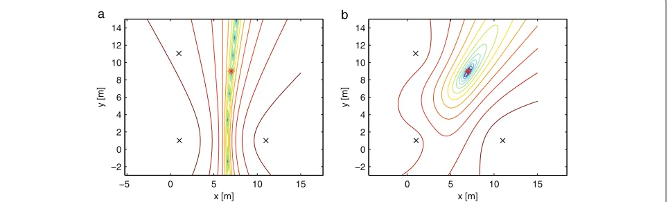
As an example, assume that nodes 1, 2, and 3 are anchors and nodeN as a passive receiving node. Then, given the sequenceT1 = {1, 2, 3, 1}, the proposed estimator
oper-ation is described in Figure 3 for batch sizesB = 1 and
B = 2, where the cost function Vb(ϑ) in (9) is
plot-ted. From the figures, it can be seen that, when B =
1, node N cannot perform self-localization unambigu-ously, based only on the hyperbolic constraint imposed by a single difference measurement of (1), cf. time-difference-of-arrival localization [40,41]. However, when
B = 2, nodeN can perform self-localization using a sin-gle batch due to the joint imposition of two hyperbolic constraintsa.
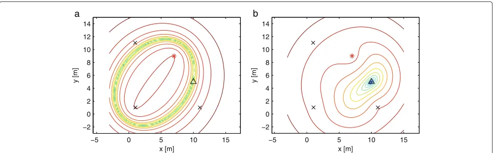
Now, let us assume that node 4 is an auxiliary node with a noninformative prior. Then, given the sequence
T2 = {1, 2, 3, 1, 4, 2, 4}, the cost functionVb(ϑ) in (9) is
illustrated in Figure 4. For batch size B = 1, node N
cannot localize auxiliary node 4 unambiguously, based only on the elliptical constraint imposed by a single time-difference measurement of (1), cf. [42]. However, as node 4 is interleaved with anchor nodes in the sequence and node
Nhas self-localized, (1) produces elliptical and hyperbolic constraints alternatingly depending on whether node i
is an anchor or auxiliary node, respectively. Hence for
B = 3, node N can localize the auxiliary node due to the joint imposition of two elliptical and one hyperbolic constraint.
The above example can easily be extended toNaanchor
nodes. Let the anchor nodes be indexed as 1, 2,. . .,Naand the auxiliary nodes asNa+1,Na+2,. . .. Then a generic sequence can be constructed on the form
Tg= { 1, 2, . . .,Na
enable self-localization
,. . ., 1,Na+k, 2,Na+k,. . . kth auxiliary node localized in this batch
,. . .},
where the kth auxiliary node is localized as long as it is interleaved by at least two anchor nodes in its
x [m]
y [m]
0 5 10 15
−2 0 2 4 6 8 10 12 14
x [m]
y [m]
−5 0 5 10 15
−2 0 2 4 6 8 10 12 14
a b
Figure 3Cost functionVb(ϑ)with respect to variablesxN, using sequenceT1= {1, 2, 3, 1}.Anchor nodes are denoted by crosses and the
x [m]
y [m]
−5 0 5 10 15
−2 0 2 4 6 8 10 12 14
x [m]
y [m]
−5 0 5 10 15
−2 0 2 4 6 8 10 12 14
a b
Figure 4Cost functionVb(ϑ)with respect to variablesx4, using sequenceT2= {1, 2, 3, 1, 4, 2, 4}.Here, anchor nodes are denoted by crosses,
the auxiliary node 4 is denoted by a triangle, and the passive receiving nodeNis denoted by an asterisk.(a)Batch sizeB=1, batch indexb=4.(b) Batch sizeB=3, batch indexb=2.
corresponding batch. Thus, for a given batch sizeB, the sequenceTgwill be padded by interleaving anchor nodes
to fulfill this constraint. Once all auxiliary nodes have been localized, the sequence is simply repeated which improves the estimates in the next round of measurements.
Finally, note that the sequential nature of the estima-tor allows for robustness to random link failures. In fact, in the event of a lost measurement, the corresponding batch is discarded and the estimator proceeds with the subsequent batches.
4 Numerical results
In this section, we provide a numerical performance eval-uation of the estimator derived in section 3. As a case study, we consider the two-dimensional localization of nodes in an IR-UWB wireless sensor network [11,18,28]. In such a scenario, the timing information is obtained by measuring the propagation time of subnanosecond UWB pulses. The measurement noise is generated according to numerical values that are consistent with this scenario, i.e. subnanosecond- to nanosecond-order standard deviation, based on the experimental characterization in [18-21].
We analyze the localization of all nodes in the network performed at a passive receiver node. The analysis is appli-cable in a straightforward manner to any transceiver node which participates in the sequence.
Reproducible research:Code for reproducing results in this section is provided at the webpage of KTH Signal Processing, under ‘reproducible research’ http://www.kth. se/en/ees/omskolan/organisation/avdelningar/sp/research /reproducibleresearch-1.433797.
4.1 Setup
We consider a fully connected network ofNnodes con-sisting ofNa = 4 anchors andNu = N−Naunknown
position nodes. The latter includes one passive receiver node, which we denote as self-localizing node, andNu−1
auxiliary nodes, i.e., transceiver nodes with noninforma-tive prior which participate in the transmission sequence. We assume that the anchors are deployed according to nominal positions affected by a Gaussian error with a known covariance Pθa = σa2I2Na. The remaining nodes
have noninformative priors, i.e.,P−θu1 = 0, and the delay δihas a nominal value ofμδ = 10−6s with known error varianceσδ2.
In the numerical simulations, we consider a total ofM
samples. Except where otherwise indicated, the noise is generated asw∼N(0,σ2Q), where
Q= ⎡ ⎢ ⎢ ⎢ ⎢ ⎢ ⎣
q1 1/3 1/3 q2 1/3
1/3 q3 1/3 . .. ... 1/3
1/3 qM
⎤ ⎥ ⎥ ⎥ ⎥ ⎥ ⎦∈R
M×M (14)
andqi=1,∀i.
The transmission sequenceT is constructed by inter-leaving the transmissions from the auxiliary nodes with those of anchors, according to the approach described in section 3.3. Furthermore, the batch length is set to
B=7, which enables localization using allNa=4 anchors
within the same batch.
We initialize the AMAP estimator of Algorithm 1 with
μ=[μ1 · · ·μN
a μ¯
1 · · · ¯μNu μδ1
N−1], whereμis are the
nominal anchor positions andμ¯i ≡(1/Na)Nj=a1μjis the
centroid of the nominal anchor positions. Furthermore, we set the termination criterionε=10−2Nuexcept where
The average RMSE of the position and delay estimates is the RMSE from 103Monte Carlo iterations.
4.2 Cramér-Rao bound
The mean square error when using the complete set of
M samples, y = h(ϑ) + w ∈ RM, is constrained by the Cramér-Rao bound [39]. Here we derive the bound when the noise covariance matrix equalsσ2Qas of (14) [17]. Note, however, that the covariance structureQis not given in the AMAP estimator; hence, the bound is opti-mistic and may not be attainable. Nevertheless, the bound provides a benchmark for evaluating the performance of the proposed estimator.
Letη[θδ σ2]∈RT+1, then we treat the param-eters with noninformative priors as deterministic quan-tities. Suppose ηˆ be any estimator that is conditionally unbiased with respect to the deterministic parameters. Then its mean square error (MSE) matrix is constrained by the hybrid Cramér-Rao bound (HCRB) [43],Cη˜ J−η1, whereJη=JDη +JPη ∈R(T+1)×(T+1).
Here,JDη =Eη¯[JD(η)] is the expected Fisher information matrix, whereη¯denotes the subset of parameters that are modeled as random quantities and
[JD(η)]i,j=
as given in [39]. As the expectation does not have a closed form solution, we evaluate it by the Monte Carlo simula-tion. If a subset of node positions,θu, and the noise level, σ2, are treated as deterministic and unknown parame-ters, and the remaining parameparame-ters,θaandδ, are random Gaussian, then the prior information matrix is given by
JPη=
ing, we use this division between deterministic and ran-dom parameters to study practical configurations where we lack prior knowledge on the position of a subset of nodes.
4.3 Error analysis
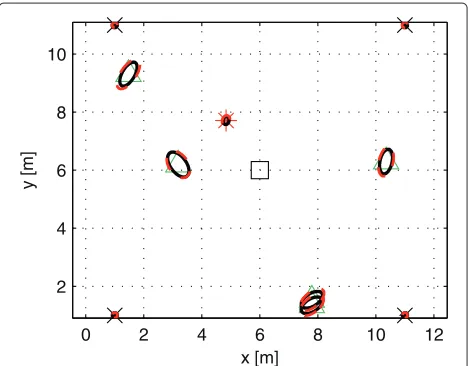
We analyze the node deployment shown in Figure 5, where the nominal positions of the anchors are the cor-ners of a 10 × 10 m2 area. The positions of the five
auxiliary nodes and of the self-localizing nodes are ran-domly generated according to a uniform distribution within this area. Here,Nu =6 and we use a transmission
sequenceT with|T| =71.
The performance of the proposed estimator is com-pared with the HCRB by means of error ellipses. For visual clarity, the sizes of the ellipses have been scaled to corre-spond to 99% confidence ellipses of a zero-mean Gaussian distribution [16].
In Figure 5, a highly informative prior on the anchor positions, of centimeter level, is used. Further, in Figure 6, a relatively less informative prior is employed, i.e., a decimeter-level prior, to model uncertainty in the deploy-ment of the anchors in a practical scenario. It can be seen that the proposed AMAP estimator is close to the HCRB in both cases. In both cases, the gap between the average RMSE and the HCRB is less than 2 cm. Thus, the esti-mator is inherently robust with respect to anchor position uncertainty.
In Figures 5 and 6, the ellipses related to the self-localizing node are considerably smaller than those of the auxiliary nodes, and are of the same order of mag-nitude as the prior on the anchor positions. Further, the minor axes of the ellipses of the auxiliary nodes are approximately aligned along the direction connecting to
0 2 4 6 8 10 12
0 2 4 6 8 10 12 2
4 6 8 10
x [m]
y [m]
Figure 6True node positions and error ellipses for the same node deployment as that in Figure 5.Here,σa=30 cm and σ=1 ns. The average RMSE of the position estimate is 13.2 cm and the HCRB is 11.5 cm.
the self-localizing node. This phenomenon, previously observed in [16], is due to the fact that the self-localizing node performs an independent measurement of its own distance to a generic nodeievery time nodeitransmits. Therefore, the self-localization performance is improved at every measurement, and the error variance of the posi-tion estimate for node i is reduced along the direction connecting it to the self-localizing node.
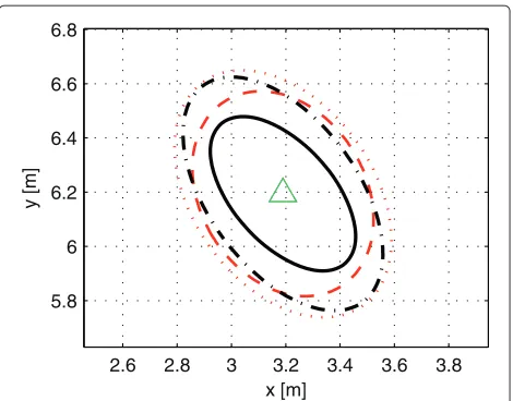
Moreover, from the magnified comparison for an aux-iliary node in Figure 7, it is possible to visually analyze
2.5 3 3.5 4
5.6 5.8 6 6.2 6.4 6.6 6.8
x [m]
y [m]
Figure 7Error ellipses of a single auxiliary node in the scenario of Figure 5, under two different values of priors of anchor positions.
The solid black ellipse is the HCRB forσa=3 cm whereas the dashed red ellipse indicates the performance of the AMAP estimator in the same scenario. The larger dash-dotted black ellipse and the dotted red ellipse indicate the HCRB and the performance of the AMAP estimator, respectively, in theσa=30 cm case. Here,σ=1 ns.
0 0.5 1 1.5 2 2.5 3
x 10−9 10−2
10−1 100
σ [s]
RMSE
θ u
[m]
HCRB, σ a = 3 cm AMAP, σa = 3 cm HCRB, σa = 30 cm AMAP, σa = 30 cm
Figure 8Average RMSE of the position estimate vs noise level under different anchor position priors.Here,σδ=100 ps.
the effect of the anchor position priors on the perfor-mance. In particular, the ratio between the major and minor axes of both the HCRB and MSE ellipses decreases when the the prior becomes less informative. This is due to the increased error in the estimate of the self-localizing node position, which causes poorer performance in the direction connecting every auxiliary node and the self-localizing node.
4.4 Error statistics
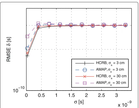
We now provide a statistical performance evaluation of the position and delay estimates as a function of the noise level, which is parameterized byσ. The simulation results, obtained using the same network configuration as that of Figure 5, are shown in Figures 8, 9, 10, and 11, where
0 0.5 1 1.5 2 2.5 3
x 10−9 10−10
σ [s]
RMSE
δ
[s]
HCRB, σa = 3 cm AMAP, σa = 3 cm HCRB, σa = 30 cm AMAP, σa = 30 cm
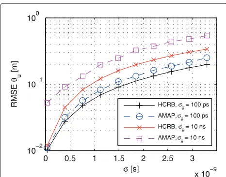
0 0.5 1 1.5 2 2.5 3
x 10−9 10−2
10−1 100
σ [s]
RMSE
θ u
[m]
HCRB, σδ = 100 ps AMAP, σδ = 100 ps HCRB, σδ = 10 ns AMAP, σδ = 10 ns
Figure 10Average RMSE of the position estimate vs noise level under different delay priors.Here,σa=3 cm.
different priors for the anchor positions and the delay are used.
Specifically, in Figures 8 and 9, the uncertainty of the anchor positions, parameterized by σa, is varied from
centimeter-level to decimeter-level. It is possible to notice that, in low noise conditions, the RMSE of the position estimation is of the same order of magnitude as the uncer-tainty of the anchor positions. Also, as shown in Figure 9, the delay estimator achieves a performance close to the HCRB, and is robust with respect to parameter uncer-tainty in the anchor positions.
Moreover, the parameterσδ, related to the uncertainty in the delay, is varied over two orders of magnitude in Figures 10 and 11. The results show that the proposed
0 0.5 1 1.5 2 2.5 3
x 10−9 10−12
10−11 10−10 10−9 10−8 10−7
σ [s]
RMSE
δ
[s]
HCRB, σδ = 100 ps AMAP, σδ = 100 ps HCRB, σδ = 10 ns AMAP, σδ = 10 ns
Figure 11Average RMSE of the delay estimate vs noise level under different delay priors.Here,σa=3 cm.
AMAP estimator is also robust with respect to uncertainty in the delay.
The behavior of the estimator with respect to the length of the transmission sequence is shown in Figure 12. The different sequence lengths in the figure are obtained by repeating T. Two values of the batch length B are reported. As expected, the performance improves as the length of the sequence increases. It can also be noticed that the performance of the proposed AMAP estimator improves as the batch length increases, given a fixed sequence length. This improvement establishes a performance trade-off since it comes at the expense of a reduced update rate of the system.
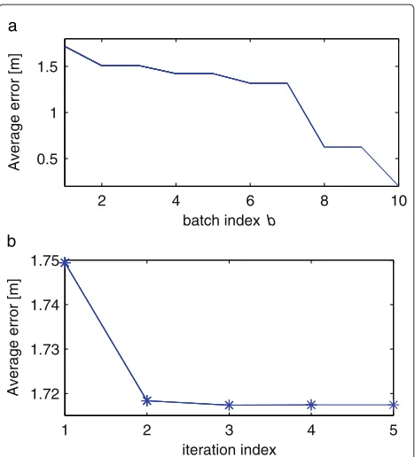
4.5 Convergence evaluation
In order to analyze the convergence behavior of the pro-posed estimator, we evaluate simulation results obtained in the loose-prior scenario of Figure 6, where we set the termination threshold = 10−5Nu. Figure 13a shows
the behavior of the proposed estimator in a realization of the transmission sequence T. It can be noticed that the error decreases at each batch within the sequence, as each auxiliary node is successfully localized.
Furthermore, Figure 13b shows a sample realization of the iteration at line 3 of Algorithm 1 during the first batch. The error decreases monotonically with the number of iterations.
A histogram of the number of iterations until conver-gence for the first batch is shown in Figure 14a. The aver-age number of iterations is 5.54. With=10−2Nu, which
yields negligible RMSE performance loss, the histogram is shown in Figure 14b and we observe an average num-ber of iterations of 3.71. Finally, simulation results show that the inner loop of line 8 in Algorithm 1 exhibits a fast
0 200 400 600 800
0.02 0.03 0.04 0.05 0.06 0.07 0.08
sequence length [number of transmissions]
RMSE [m]
RMSE, B = 7 RMSE, B = 15 HCRB
1 2 3 4 5 1.72
1.73 1.74 1.75
iteration index
Average error [m]
2 4 6 8 10
0.5 1 1.5
batch index b
Average error [m]
a
b
Figure 13Error behavior of proposed AMAP estimator, in sample realization.With respect to(a)batch indexbwithin sequenceT and (b)iteration indexforb=1. Here, the average error is defined as 1/Nuθu− ˆθu.
0 5 10 15 20 25
0 200 400 600
Number of iterations until convergence
Count
1 2 3 4 5 6 7 8 9 10
0 200 400 600
Number of iterations until convergence
Count
a
b
Figure 14Convergence behavior for two values of stopping criterion : (a) =10−5N
u.(b) =10−2Nu.
convergence behavior with an average of approximately 1.23 iterations.
4.6 Large-scale setup
In order to provide insight on the scalability of the pro-posed estimator, we present an extensive scenario in Figure 15. We considerN = 29 nodes, includingNa = 4
anchors in the same nominal positions as the previous sce-nario of Figure 5, andNu =25 unknown position nodes.
The positions of the latter are generated by adding noise uniformly distributed in a square region with an area of 1 m2to a fixed 5×5 grid of evenly distributed nodes. A transmission sequence T, withT = 337 is used, and the batch size is set toB = 7. The figure shows that the proposed method is capable of localizing 24 auxiliary nodes with an accuracy of the same order of magnitude as the considered anchors position prior.
4.7 Noise outliers
To evaluate the effect of varying noise levels on the proposed AMAP estimator, we generate noise as w ∼ N(0,σ2Q), where Q is fixed and given by (14), but in which we set
qi=
1 with probability 0.9
100 with probability 0.1 ∀i (15)
Such a noise model is equivalent to randomly picking 10% of the observations and assigning a standard deviation σoutl = 10σ to the noise affecting those observations. As
0 2 4 6 8 10 12
2 4 6 8 10
x [m]
y [m]
Figure 15Large-scale setup on a 5×5 grid of unknown position nodes.Each of the nominal positions is randomized by adding a random variable which is uniformly distributed in a square region with an area of 1 m2. Here,σ=1 ns,σa=3 cm, andσδ=100 ps.
0 20 40 60 80 100 −25
−20 −15 −10 −5 0 5 10 15 20
Sample index m
timing error [ns]
Figure 16Realization of Gaussian noise having a standard deviation ofσ=1ns, which is affected by10%of outliers with σoutl=10σ.
an illustrative example, one realization ofw is shown in Figure 16.
Figure 17 shows the behavior of the AMAP estimator when the outlier measurement noise model is considered, whereas a magnification of the error ellipses for one auxil-iary node is shown in Figure 18. The results show that the proposed estimator is still operational and capable of pro-viding accurate results even in the presence of relatively large outliers.
5 Conclusion
We considered the schedule based network localization concept, proposed in [15-17]. This concept does away with the need for synchronization among nodes and does
0 2 4 6 8 10 12
2 4 6 8 10
x [m]
y [m]
Figure 17HCRB and MSE ellipses in the presence of outliers.
The RMSE of the proposed AMAP estimator is 9.3 cm and the HCRB is 4.7 cm.
2.6 2.8 3 3.2 3.4 3.6 3.8 5.8
6 6.2 6.4 6.6 6.8
x [m]
y [m]
Figure 18Error ellipses of single auxiliary node.Ellipses show effect of error outliers on HCRB and AMAP performance in scenario of Figure 5. Solid black and dashed red ellipses and for the outliers case, dash-dotted black ellipse and dotted red ellipse.
not involve communication overhead. It utilizes a com-mon transmission sequence, which enables each node to perform joint self- and network localization, based on noisy propagation time measurements. The schedule-based localization problem has been posed as an esti-mation problem with probabilistic prior inforesti-mation. We derived a sequential estimator, AMAP, which is fully decentralized and copes with varying noise levels. The estimator is robust with respect to uncertainty in anchor locations and delay.
The measurement model we considered contains well-established constraints in the positioning literature, i.e., circular, hyperbolic, and elliptical constraints. The analy-sis of such constraints provides a schedule design method-ology which enables a scalable solution. Specifically, the system can localize a large number of transceiving nodes with unknown positions by building transmission sequence batches in which such nodes are interleaved with anchor nodes. Numerical results in an IR-UWB net-work scenario show that AMAP provides localization accuracy close to a HCRB matched to the problem. Fur-thermore, AMAP is shown to be robust with respect to noise outliers.
Endnote
aIf nodeNis participating in the sequence, it also gives
rise to circular constraints which are analogous to those provided by the two-way TOA technique [29].
Competing interests
The authors declare that they have no competing interests.
Acknowledgements
Author details
1ACCESS Linnaeus Centre, Signal Processing Lab, KTH Royal Institute of
Technology, Stockholm, Sweden.2Current address: Department of Information Technology, Uppsala University, Uppsala, Sweden.3Current address: Department of Electronic and Information Engineering, University of Perugia, Perugia, Italy.
Received: 30 May 2013 Accepted: 15 January 2014 Published: 6 February 2014
References
1. N Patwari, J Ash, S Kyperountas, A Hero III, R Moses, N Correal, Locating the nodes: cooperative localization in wireless sensor networks. IEEE Signal Process. Mag.22(4), 54–69 (2005)
2. J Rantakokko, J Rydell, P Stromback, P Handel, J Callmer, D Tornqvist, F Gustafsson, M Jobs, M Grudén, Accurate and reliable soldier and first responder indoor positioning: multisensor systems and cooperative localization. Wireless Commun. IEEE.18(2), 10–18 (2011)
3. H Liu, H Darabi, P Banerjee, J Liu, Survey of wireless indoor positioning techniques and systems. IEEE Trans. Syst., Man, Cybernet., Part C: Appl. Rev.37(6), 1067–1080 (2007)
4. G Mao, B Fidan, B Anderson, Wireless sensor network localization techniques. Comput. Netw.51(10), 2529–2553 (2007)
5. K Lui, WK Ma, H So, F Chan, Semi-definite programming algorithms for sensor network node localization with uncertainties in anchor positions and/or propagation speed. IEEE Trans. Signal Process.
57(2), 752–763 (2009)
6. G Shirazi, M Shenouda, L Lampe, Second order cone programming for sensor network localization with anchor position uncertainty, in Proceedings on Workshop on Positioning Navigation and Communication (WPNC)(Dresden, Germany, 7-8 April 2011), pp. 51–55
7. J Zheng, YC Wu, Joint time synchronization and localization of an unknown node in wireless sensor networks. IEEE Trans. Signal Process. 58(3), 1309–1320 (2010)
8. M Gholami, S Gezici, E Strom, TDOA based positioning in the presence of unknown clock skew. IEEE Trans. Commun.61(6), 2522–2534 (2013) 9. M Win, A Conti, S Mazuelas, Y Shen, W Gifford, D Dardari, M Chiani,
Network localization and navigation via cooperation. IEEE Commun. Mag. 49(5), 56–62 (2011)
10. Y Shen, M Win, Fundamental limits of wideband localization - Part I: A general framework. IEEE Trans. Inform. Theory56(10), 4956–4980 (2010) 11. H Wymeersch, J Lien, M Win, Cooperative localization in wireless
networks. Proceedings of IEEE.97(2), 427–450 (2009)
12. V Savic, S Zazo, Nonparametric generalized belief propagation based on pseudo-junction tree for cooperative localization in wireless networks. EURASIP J. Adv. Signal Process.2013, 16 (2013)
13. AT Ihler, JW Fisher III, RL Moses, AS Willsky, Nonparametric belief propagation for self-localization of sensor networks. Select. Areas Commun. IEEE J.23(4), 809–819 (2005)
14. N Patwari, AO Hero III, M Perkins, NS Correal, RJ O’dea, Relative location estimation in wireless sensor networks. Signal Process., IEEE Trans. 51(8), 2137–2148 (2003)
15. S Dwivedi, A De Angelis, P Händel, Scheduled UWB pulse transmissions for cooperative localization, inProceedings of the IEEE Int. Conf. Ultra-Wideband (ICUWB)(Syracuse, New York, 17-20 Sept. 2012), pp. 6–10 16. S Dwivedi, D Zachariah, A De Angelis, P Händel, Cooperative
decentralized localization using scheduled wireless transmissions. IEEE Commun. Lett.17(6), 1240–1243 (2013)
17. D Zachariah, A De Angelis, S Dwivedi, P Handel, Self-localization of asynchronous wireless nodes with parameter uncertainties. IEEE Signal Process. Lett.20(6), 551–554 (2013)
18. A De Angelis, S Dwivedi, P Händel, Characterization of a flexible UWB sensor for indoor localization. IEEE Trans. Instrum. Meas.
62(5), 905–913 (2013)
19. A De Angelis, S Dwivedi, P Handel, Development of a radio front end for a UWB ranging embedded test bed, inProceedings of IEEE Int. Conf. Ultra-Wideband (ICUWB)(Syracuse, New York, 17-20 Sept. 2012), pp. 31–35 20. A De Angelis, S Dwivedi, P Händel, Development of a test bed for UWB
radio indoor localization of first responders, inIEEE/ION Position Location and Navigation Symposium (PLANS)(Grande Dunes, Myrtle Beach, SC, 23-26 April 2012), pp. 1106–1110
21. A De Angelis, J Nilsson, I Skog, P Händel, P Carbone, Indoor positioning by ultrawide band radio aided inertial navigation. Metrol. Meas. Syst. 17(3), 12 (2010)
22. JO Nilsson, D Zachariah, I Skog, P Händel, Cooperative localization by dual foot-mounted inertial sensors and inter-agent ranging. EURASIP Journal on Advances in Signal Processing.2013, 164 (2013)
23. M Ciurana, Arroyo Barcelo-F, F Izquierdo, A ranging method with IEEE 802.11 data frames for indoor localization, inProceedings on IEEE Wireless Comm. and Networking Conf. (WCNC)(Hong Kong, China, 11-15 March 2007), pp. 2092–2096
24. G Santinelli, R Giglietti, A Moschitta, Self-calibrating indoor positioning system based on ZigBee devices, inIEEE Instrumentation and Measurement Technology Conference, I2MTC(Singapore, 5-7 May 2009), pp. 1205–1210 25. M Pichler, S Schwarzer, A Stelzer, M Vossiek, Multi-channel distance
measurement with IEEE 802.15. 4 (ZigBee) devices. IEEE J. Select. Topics Signal Process.3(5), 845–859 (2009)
26. J Wang, Q Gao, Y Yu, H Wang, M Jin, Toward robust indoor localization based on Bayesian filter using chirp-spread-spectrum ranging. Industrial Electron., IEEE Trans.59(3), 1622–1629 (2012)
27. M Win, R Scholtz, Impulse radio: how it works. IEEE Commun. Lett. 2(2), 36–38 (1998)
28. A Conti, M Guerra, D Dardari, N Decarli, MZ Win, Network experimentation for cooperative localization. IEEE J. Select. Areas Commun.30(2), 467–475 (2012)
29. S Gezici, Z Tian, G Giannakis, H Kobayashi, A Molisch, H Poor, Z Sahinoglu, Localization via ultra-wideband radios: a look at positioning aspects for future sensor networks. IEEE Signal Process. Mag.22(4), 70–84 (2005) 30. S Gezici, H Poor, Position estimation via ultra-wide-band signals.
Proceedings of IEEE.97(2), 386–403 (2009)
31. D Dardari, A Conti, U Ferner, A Giorgetti, M Win, Ranging with ultrawide bandwidth signals in multipath environments. Proceedings of the IEEE. 97(2), 404–426 (2009)
32. D Cassioli, M Win, A Molisch, The ultra-wide bandwidth indoor channel: from statistical model to simulations. IEEE J. Select. Areas Commun. 20(6), 1247–1257 (2002)
33. A Molisch, Ultra-wide-band propagation channels. Proceedings of the IEEE.97(2), 353–371 (2009)
34. G Garcia, L Muppirisetty, H Wymeersch, On the trade-off between accuracy and delay in UWB navigation. IEEE Commun. Lett. 17, 39–42 (2013)
35. M Gholami, S Gezici, E Ström, Improved position estimation using hybrid tw-toa and tdoa in cooperative networks. IEEE Trans. Signal Process. 60(7), 3770–3785 (2012)
36. E Larsson, Cramér-Rao bound analysis of distributed positioning in sensor networks. IEEE Signal Process. Lett.11(3), 334–337 (2004)
37. S Park, E Serpedin, K Qaraqe, Gaussian assumption: the least favorable but the most useful [Lecture Notes]. IEEE Signal Process. Mag.30(3), 183–186 (2013)
38. GC Tiao, A Zellner, On the Bayesian estimation of multivariate regression. J R. Stat. Soc. Series B.26(2), 277–285 (1964)
39. SM Kay,Fundamentals of Statistical Signal Processing: Estimation Theory, vol. 1 (Prentice Hall, Englewood Cliffs, 1993)
40. P Stoica, J Li, Lecture notes: source localization from range-difference measurements. IEEE Signal Process. Mag.23(6), 63–66 (2006) 41. A Beck, P Stoica, J Li, Exact and approximate solutions of source
localization problems. IEEE Trans. Signal Process.56(5), 1770–1778 (2008) 42. Y Zhou, CL Law, YL Guan, F Chin, Indoor elliptical localization based on
asynchronous UWB range measurement. IEEE Trans. Instrumentation Meas.60, 248–257 (2011)
43. H Van Trees,Optimum Array Processing(Wiley-Interscience, New York, 2002)
doi:10.1186/1687-6180-2014-16