Significant Error Propagation in the Finite Difference Solution of Non-Linear Magnetostatic Problems Utilizing Boundary Condition of the Third Kind

SIGNIFICANT ERROR PROPAGATION IN THE FINITE

DIFFERENCE SOLUTION OF NON-LINEAR

MAGNETOSTATIC

PROBLEMS UTILIZING

BOUNDARY CONDITION OF THE

THIRD KIND

E. Afjei

Department of Electrical and Computer Engineering, Shahid Beheshti University Tehran, Iran, [email protected]

J. Rashed-Mohassel

Department of Electrical and Computer Engineering, University of Tehran Tehran, Iran, [email protected]

M. H. Arbab

Department of Electrical and Computer Engineering, Shahid Beheshti University Tehran, Iran, [email protected]

(Received: May 10, 2003 – Accepted in Revised Form: November 5, 2003)

Abstract This paper poses two magnetostatic problems in cylindrical coordinates with different permeabilities for each region. In the first problem the boundary condition of the second kind is used while in the second one, the boundary condition of the third kind is utilized. These problems are solved using the finite element and finite difference methods. In second problem, the results of the finite difference method show low magnetic vector potential as well as the magnetic field density when compared to the finite element results and in the linear case, to the analytical solution. This paper investigates the reason behind the low magnetostatic field computation in cylindrical coordinates using the finite difference method when boundary condition of the third kind is used. It then, presents a technique to overcome the problem of low magnetic field calculation using the finite difference method. The results obtained by the new technique are in close agreement with the finite element method as well as the analytical solution. Finally, it analyzes the possible source of error in modeling magnetostatic boundary conditions in finite difference formulation of vector Poisson or Laplace’s equation in cylindrical coordinates.

Key Words Nonlinear Magnetic Field, Finite Difference, Finite Element, Electromagnetics

ﻩﺪﻴﮑﭼ

ﻩﺪﻴﮑﭼ

ﻩﺪﻴﮑﭼ

ﻩﺪﻴﮑﭼ

ﺖﺳﺍﻩﺪﺷﻲﺳﺭﺮﺑﻪﻴﺣﺎﻧﻭﺩﺭﺩﺕﻭﺎﻔﺘﻣﻲﻳﺍﻭﺍﺮﺗﺎﺑﻱﺍﻪﻧﺍﻮﺘﺳﺍﻚﻴﺗﺎﺘﺳﺍﻮﺘﻨﮕﻣﻪﻟﺎﺴﻣﻪﻟﺎﻘﻣﻦﻳﺍﺭﺩ

.

ﻥﺎﺸﻧ

ﻱﺍﺮﺑ ﺩﻭﺪﺤﻣﺀﺍﺰﺟﺍ ﺵﻭﺭﺦﺳﺎﭘﺎﺑ ﺩﻭﺪﺤﻣﻞﺿﺎﻔﺗ ﺵﻭﺭﺦﺳﺎﭘ ،ﻡﻭﺩ ﻉﻮﻧﻱﺯﺮﻣ ﻂﻳﺍﺮﺷ ﺎﺑ ﻪﻛ ﺖﺳﺍ ﻩﺪﺷ ﻩﺩﺍﺩ

ﻲﺑ ﻲﻨﺤﻨﻣ ﻲﻄﺧﺮﻴﻏﻭﻲﻄﺧﻲﺣﺍﻮﻧ

ﺪﺷﺎﺑ ﻲﻣﻥﺎﺴﻜﻳﭺﺍ

.

ﺷﻪﻛﻲﺘﻟﺎﺣ ﺭﺩﺎﻣﺍ

،ﺖﺳﺍﻡﻮﺳﻉﻮﻧﺯﺍﻱﺯﺮﻣﻁﺮ

،ﺩﻭﺪﺤﻣ ﺀﺍﺰﺟﺍ ﺦﺳﺎﭘﺎﺑ ﻪﺴﻳﺎﻘﻣ ﺭﺩ ﻲﺴﻴﻃﺎﻨﻐﻣ ﺭﺎﺷ ﻲﻟﺎﮕﭼﻭ ﻲﺴﻴﻃﺎﻨﻐﻣ ﻞﻴﺴﻧﺎﺘﭘ ﻱﺍﺮﺑ ﺩﻭﺪﺤﻣﻱﺎﻬﺗﻭﺎﻔﺗ ﺦﺳﺎﭘ

ﺖﺳﺍﺩﺎﻳﺯ ﺩﻭﺪﺤﻣﺕﻭﺎﻔﺗﺵﻭﺭﺭﺩﺩﻮﺟﻮﻣﻱﺎﻄﺧﻭﺩﺭﺍﺩ ﻱﺍﻪﻈﺣﻼﻣﻞﺑﺎﻗﻑﻼﺘﺧﺍ

. ﻱﺍﺮﺑﻲﺷﻭﺭ،ﻪﻟﺎﻘﻣﻦﻳﺍﺭﺩ

ﺪﺷﻪﺋﺍﺭﺍﻲﺴﻴﻃﺎﻨﻐﻣﻥﺍﺪﻴﻣﺭﺩﻩﺪﺷﺩﺎﻳﻱﺎﻄﺧﺡﻼﺻﺍ ﺖﺳﺍﻩ

. ﺭﺎﻴﺴﺑﺩﻭﺪﺤﻣﻱﺍﺰﺟﺍﻩﻮﻴﺷﺦﺳﺎﭘﻪﺑﺵﻭﺭﻦﻳﺍﺞﻳﺎﺘﻧ

ﺩﺭﺍﺩ ﺖﻘﺑﺎﻄﻣ ﺰﻴﻧﻲﻠﻴﻠﺤﺗ ﻱﺎﻬﺑﺍﻮﺟ ﺎﺑﻭﻩﺩﻮﺑ ﻚﻳﺩﺰﻧ

. ﻱﺯﺮﻣ ﻂﻳﺍﺮﺷﻱﺯﺎﺴﻟﺪﻣ ﺭﺩﺎﻄﺧ ﻲﻟﺎﻤﺘﺣﺍﻊﺒﻨﻣ ﺖﻳﺎﻬﻧﺭﺩ

ﻞﻴﻠﺤﺗﻱﺍﻪﻧﺍﻮﺘﺳﺍﺕﺎﺼﺘﺨﻣﺭﺩﺱﻼﭘﻻﻭﻥﻮﺳﺍﻮﭘﻱﺭﺍﺩﺮﺑﻪﻟﺩﺎﻌﻣﺭﺩﺩﻭﺪﺤﻣﺕﻭﺎﻔﺗﻱﺪﻨﺒﻟﻮﻣﺮﻓﺎﺑﻲﻜﻴﺗﺎﺘﺳﺍﻮﺘﻨﮕﻣ ﺖﺳﺍﻩﺪﺷ

.

1. INTRODUCTION

In this paper, the nonlinear magnetic field calculation

the inadequacy in the finite difference method is outlined. Afjei and Rashed have addressed the problem of inadequacies in finite difference solution of magnetic field in [1] for a linear case and outlined a procedure to fix this problem. The comparison of the first-order finite element and finite difference algorithms for the analysis of the magnetic field problems has been mentioned in [2-3]. The computation of magnetostatic field problems using the finite element technique as well as the finite difference method in Cartesian coordinates can be found immensely in the literature [4-7]. Now days computer packages using the finite element methods are available in the market which computes the

magnetic field problems in all sorts of shape and geometry[8]. In this paper two case studies have been discussed. In the first case, a long current carrying conductor is considered with a relatively high permeable material (M-19: USS Transformer 72 ... 29 gage) surrounding the conductor where the boundary conditions are of the second kind. The second case considers a long core having the same high permeable material as problem one, with a coil wrapped around it. In this case the boundary conditions are of the third kind. These problems are solved by two different methods namely the finite element method and the finite difference technique and the results of both problems are then compared.

2. CALCULATION OF B-FIELD IN THREE CONCENTRIC CIRCLES

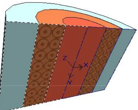
Consider a long current carrying conductor with a high permeable material surrounding the conductor. A cut view of the current carrying conductor and it’s surrounding plus the corresponding cross section of the geometry is shown in Figure 1.

There are three concentric circles with different relative permeabilities. The center circle, which is a conductor, has a radius of ra =1 Cm, the relative

permeability of this region is one with a current density, Jz. Region two, which is made up of high

permeable magnetic material (M-19: USS Transformer 72 ... 29 gage), has a radius of rb = 3Cm. with the

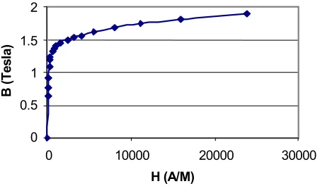
B-H curve shown in Figure 2.

Region 3, the surrounding medium, is the free space having a radius of rc = 6 Cm.

In order to analyze the magnetic field in these regions, recognizing the low frequency nature of the problem, static field calculation has been performed. The static B-H curve has been broken into 5 different second order polynomials for the analysis. The corresponding vector potential equation is [9];

J

)

A

(

) B (

=

µ

×

∇

×

∇

where, µ( B ) is the permeability of the region at some

Figure 1. A cut view of the current carrying conductor and its surrounding.

0 0.5 1 1.5 2

0 10000 20000 30000

H (A/M)

B (

T

es

la

)

radius, r.

Due to symmetrical nature of the magnetic field, this problem can be simplified to a one-dimensional problem by realizing _∂Az / ∂θ and ∂Az

/ _∂z are all zeroes.

Since the current is z-directed, Equation 1 becomes a scalar Poisson's equation in z-direction and, in cylindrical coordinate can be written as [10];

J )) r A ( r 1 ( r r

1 z

B

− = ∂ ∂ µ ∂

∂ ₍₂₎

We seek the solution to the Poisson's equation in region one and the Laplace's Equation is solved for regions two and three along with the appropriate boundary conditions. The appropriate boundary condition in terms of the vector potential results

Figure 3. Magnetic field density versus radius for different current magnitudes (Finite Element).

from the continuity of the tangential component of magnetic field strength:

.

r

A

1

=

r

A

1

2 z

1













∂

∂

µ













∂

∂

µ

The above boundary condition is used at the interface of the first and the second regions, as well as the second and third regions. The outer boundary condition is

Az Irmax = 0 (4)

This technique results in a solution for the vector potential, Az. The magnetic flux density, B, then

can be calculated by,

A

x

=

B

∇

In the finite element technique, the variational method (Ritz) is employed to solve the cylindrical

0

0.25

0.5

0.75

1

1.25

1.5

0

0.01

0.02

0.03

0.04

0.05

0.06

Radius (m)

M

ag

n

et

ic

Fi

el

d D

ensi

ty

(

T)

I

=

100

A

I

=

10

A

i

=

1

A

Figure 5. Magnetic field density vs. radius for different current magnitudes (Finite Difference).

0.0

E

+

00

5.0

E

-

03

1.0

E

-

02

1.5

E

-

02

2.0

E

-

02

2.5

E

-

02

3.0

E

-

02

0

0.01

0.02

0.03

0.04

0.05

0.06

Radius (m)

Ma

gn

eti

c V

ec

to

r P

ote

n

tia

l

I

=

100

A

I

=

10

A

I

=

1

A

form of vector Poisson's equation shown in 2. In the variational method, the solution to the partial differential Equation 2 obtained in r-direction by minimizing the following functional [10-11];

∫

∫

−





























µ

=

dr

rJ

Adr

dr

dA

r

2

1

)

A

(

F

2

) B (

(6)

The corresponding elemental stiffness matrix as well as the force vector for each element can be written as ;

1,2

=

j

i,

]rdr

dr

(r)

dN

dr

(r)

dN

[

1

=

K

) B ( r

r ij

1

2

µ

∫

∫

=

2

r

r

z i

i

=

rN

(

r

)

J

dr

i

1

,

2

F

In order to solve this problem, a constant µ (B) from

the linear part of the B-H curve is chosen for the core material and sets of simultaneous algebraic equations are formed by utilizing Equation 7 for all elements. The sets are then solved and from the solution new µ (B) calculated. The new µ (B) inserted

into Equation 7 and other sets are formed, solved and a newer µ (B) computed. This process repeated

until the difference in µ (B) from the last iteration

with the one before that is less than some acceptable tolerance. It is noteworthy to mention that, the static B-H curve has been broken into 5 different second order polynomials for the analysis and used in the computation.

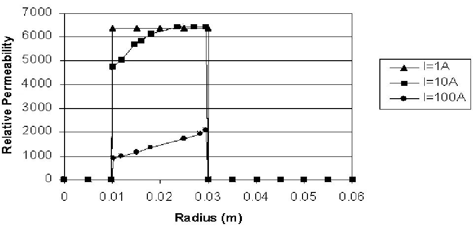
The plots of the magnetic field density, B, using the finite element technique as well as, the corresponding relative permeability for different current magnitudes from linear to fully non-linear cases are shown in Figure 3 and 4, respectively. As seen from the above Figures, the plots are linear for 1A of current, then there is local saturation in the steel for 10A case, and finally for 100A study, the steel part of the medium has gone into full saturation. The results obtained for the magnetic field density and the magnetic vector potential from the finite difference method are shown in Figures 5 and 6, respectively.

A comparison of these results obtained by the finite difference and the finite element methods show very close agreement.

3. CALCULATION OF B-FIELD IN A LONG STATOR CORE

Consider a long cylindrical steel core with a coil wrapped around it. A cut view of the coil, direction of the current in the coil, and the it’s surrounding is shown in Figure 7.

This problem consists of 3 regions. Region 1, which is made of high permeable magnetic material (M-19: USS Transformer 72 ... 29 gage), has a radius of ra = 2Cm. with the B-H curve shown in

Figure 2. Region 2 is a coil and has a current density only in θ direction (rc =4 Cm, Jθ≠0, µr=1).

Finally, region 3 is the surrounding medium, air and has a radius of rb = 6 Cm. Since this problem

is symmetric in θ-direction the vector potential has one component in this direction, and the problem can be solved in 1-dimension only. The cylindrical form of vector Poisson's equation, 1 is;

J

))]

rA

(

r

(

r

1

[

r

∂

=

−

∂

µ

∂

∂

with the following boundary conditions in terms of the vector potential in the cylindrical coordinate system;

.

r

A

+

r

A

1

=

r

A

+

r

A

1

2 2

1 1













∂

∂

µ













∂

∂

µ

θ θ

θ

θ ₍₉₎

The above boundary condition is known as the boundary condition of the third kind in which it involves the Aθ/r term. In the finite element technique, the variational method (Ritz) is employed to solve the cylindrical form of vector Poisson's equation shown in 8.

In the variational method, the solution to the

partial differential Equation 8 obtained in r direction by minimizing the following functional [10-11];

∫

∫

−





























µ

=

dr

rJ

Adr

dr

)

rA

(

d

r

1

2

1

F

2

) B (

(10)

The corresponding elemental stiffness matrix as well as the force vector for each element can be written as;

0

0.2

0.4

0.6

0.8

1

1.2

1.4

1.6

1.8

0

0.01

0.02

0.03

0.04

0.05

0.06

Radius (m)

Ma

gn

tic

F

ie

ld

D

en

sit

y

(T

)

I

=

100

A

I

=

10

A

I

=

1

A

Figure 8. Magnetic field density versus radius for different current magnitudes (Finite Element).

0

1000

2000

3000

4000

5000

6000

7000

0

0.01

0.02

0.03

0.04

0.05

0.06

Radius (m)

R

el

at

ive P

er

m

eab

ili

ty

I

=

1

A

I

=

5

A

I

=

30

A

1,2

=

j

i,

]dr

dr

(r)

dN

dr

(r)

dN

[

r

1

=

K

) B ( r

r ij

1

2

µ

∫

1,2

=

i

dr

J

(r)

Ni

r1

r2

=

Fi

∫

θ

The magnetic field, Bz, is given by

r

A

+

r

A

=

B

∂

∂

θ ₍₁₂₎

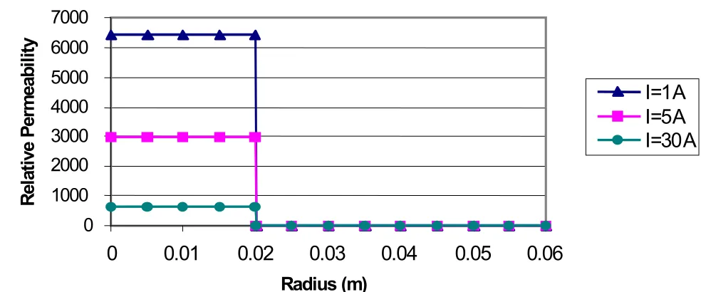
The plots of the magnetic field density, B, using the finite element technique as well as, the corresponding relative permeability for different current magnitudes from linear to fully non-linear cases are shown in Figures 8 and 9, respectively. As shown in the Figure 8 the magnetic field in

0

0.01

0.02

0.03

0.04

0.05

0.06

0.07

0.08

0

0.01

0.02

0.03

0.04

0.05

0.06

Radius (m)

Ma

gn

et

ic

Fi

el

d

De

ns

it

y (

T

)

I=30A

I=5A

I=1A

Figure 10. Magnetic field density versus radius (Finite difference).

0.0E+00

2.0E-04

4.0E-04

6.0E-04

8.0E-04

0

0.01

0.02

0.03

0.04

0.05

0.06

Radius (m)

M

ag

ne

tic

V

ec

to

r

P

ote

nt

ia

l

I=30A

I=5A

I=1A

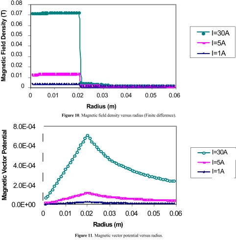
the core builds up to the maximum value and stays constant there. In Figure 9 the relative permeability has also stayed constant in the core and reduced to smaller values as the current magnitude increased. The number of turns is 5, therefore the corresponding current density for 1 A current is 3125 A/m2. The result of magnetic field density and the magnetic vector potential using the finite difference technique for different current magnitudes and sixty nodal points are shown in Figures 10 and 11,

respectively.

Comparing the plots in Figures 8 and 10 show different results for the finite element and finite difference solutions.

The discrepancy in the two results drastically increases when the relative permeability increases. It seems that the finite difference results are inaccurate when the relative permeability of the two media changes abruptly over the boundary. Now the number of grid points increased from 60

0.0E+00

5.0E-04

1.0E-03

1.5E-03

0

0.01

0.02

0.03

0.04

0.05

0.06

Radius (m)

Magneti

c Vect

or

Potent

ial

I=30A

I=5A

I=1A

Figure 12. Magnetic field density versus radius for 120 points (Finite difference).

0.0E+00

5.0E-04

1.0E-03

1.5E-03

0

0.01

0.02

0.03

0.04

0.05

0.06

Radius (m)

M

ag

ne

tic

V

ec

to

r P

ote

nt

ia

l

I=30A

I=5A

I=1A

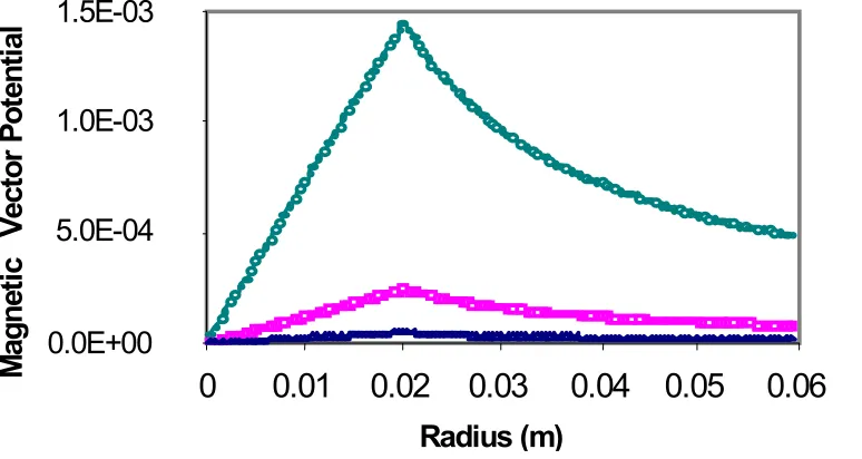
to 120 in the finite difference method and the magnetic field calculated again. Here are the results of magnetic field density and the magnetic vector potential.

The new calculation of the fields with 120 grid points shows closer results to the finite element method (but not accurate yet) when compared to the 60 grid points, therefore the error decreases as the grid point increases.

In order to verify the validity of the results, a comparison with the analytical solution should be performed.

4. ANALYTICAL SOLUTION

Since the permeability of the core stays at some constant value throughout the core region even in saturation then, Equation 8, can be transformed to a second order Cauchy-Euler equation and the analytical solution is

R

r

0

for

r

]

J

)

R

-R

(

2

[

=

A

µ

≤

≤

R r R for r 3 R J + 2 R R J -R J ) R -R ( 2 + 3 r J -r 2 R J = A c a 1 -a 3 coil a 2 c air a2 a c core 2 c air ≤ ≤     

µ µ µ

µ    µ θ r r for r ) 3 R J + 2 R R j -R J ) R -R ( 2 + 3 R J -R 2 R J ( = A c 1 -a 3 coil a 2 c air a2 a c core c 3 coil c 2 c air ≥     

µ µ µ

     µ    µ θ

where Ra is the radius of core, and Rc is the radius

of coil.

The only problem here is that, the value of µcore

is not known and cannot be calculated analytically. The magnetic field is then obtained using

r

A

+

r

A

=

B

∂

∂

θ ₍₁₄₎

can be written as;

R

r

for

0.0

=

B

R

r

R

for

J

r)

-R

(

=

B

R

r

0

for

J

)

R

-R

(

=

B

≥

≤

≤

µ

≤

≤

µ

The plots of the magnetic vector potential and the magnetic field density cannot be shown unless the value of permeability of the core material is known but the general shape of the curves is the same as the finite element method for any relative permeability value chosen from Figure 9. In the linear case, the relative permeability of the core is known to be 6500. This value is substituted in the analytical solution; the shapes of the magnetic field density and the magnetic vector potential obtained are exactly the same as the finite element method but with a drastic drop in magnitude for the finite different technique. Hence, the numerical results obtained employing the finite difference method is not reliable.

In order to investigate the problem, the analytical solution is inserted in the finite difference representation of the boundary condition.

5. FINITE DIFFERENCE APPROXIMATION OF MAGNETOSTATIC FIELD

This section analyzes a possible source of error in modeling magnetostatic boundary conditions in a finite difference formulation of vector Poisson or Laplace Equation in cylindrical coordinates. It was shown in section 3 that when magnetic fields are approximated from the vector potential using the first-order differences at the boundary, the results are in error. The error is proportional to the relative permeability of the two materials constituting the boundary. Only using an extremely fine mesh can minimize the error. The use of higher order differences can alleviate the problem, but yet the error remains proportional to relative permeability. An alternate formulation of the vector potential, in the one-dimensional case, is to make the error independent of the relative permeability of the two materials.

condition between core and coil implies









∂

∂

µ









∂

∂

θ

r

A

+

r

A

=

r

A

+

r

A

coil r

iron

(16)

at the boundary. Here µr = µcore / µ0 is the relative

permeability. In order to analyze the behavior of Equation 16, the discritization of the exact analytical

solution at the boundary is examined. Without loss of generality, assume a constant value for the permeability of the magnetic material and a uniform grid size, d meter.

The (1/r) terms in Aθ do not contribute to flux density but arises from the requirement that Aθ is continuous. It should be noted that in the coil region the (1/r) term dominates since µcore is large.

Using first order differences on either side of the

0.0E+00

2.0E-03

4.0E-03

6.0E-03

8.0E-03

1.0E-02

1.2E-02

1.4E-02

0

0.01

0.02

0.03

0.04

0.05

0.06

Radius (m)

Magneti

c

Vect

or

Potent

ial

I=30A

I=5A

I=1A

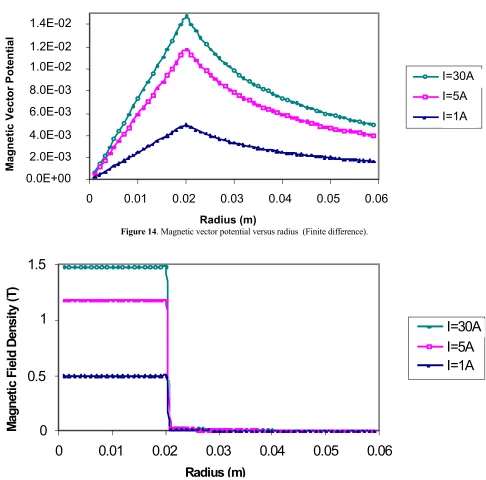
Figure 14. Magnetic vector potential versus radius (Finite difference).

0

0.5

1

1.5

0

0.01

0.02

0.03

0.04

0.05

0.06

Radius (m)

M

agn

et

ic

Fi

el

d De

ns

ity

(T

)

I=30A

I=5A

I=1A

boundary, the approximation to 16 becomes

)

d

)

r

(

A

)

d

r

(

A

r

A

(

d

)

d

r

(

A

)

r

(

A

r

)

r

(

A

r θ θ θ

θ θ θ

−

+

+

µ

=

−

−

+

Now substituting the analytical solution for Aθin 17 and simplifying it, yields;

]

k

d

k

[

core

≈

µ

µ

+

+

µ

µ

where k1, and k2 are constants.

In another words, expression in 18 can be written as;

ε

+

µ

≈

µ

where, the error is directly proportional to µcore and

incremental distance d

It is observed that for a practical range of interest the error caused by high value of µr is substantial.

Recognizing that the dominant (1/r) term is the one causing the error then, a new variable A'θ is chosen such that A'θ = r Aθ. The new formulation for the boundary condition and Laplace equations with this new variable are;









∂

′

∂

µ









∂

′

∂

r

A

=

r

A

J

))]

A

(

r

(

r

1

[

r

θ

=

−

∂

∂

µ

∂

∂

The general solution to the Equation 21 employing boundary Equation 20 is

. R r ) C + (C = A R r R r C -) C -(C + r C = A R r r C = A c 0 7 core 6 c a 3 0 5 0 4 core 3 2 0 2 a 2 core 1 ≥ µ µ ′ ≤ ≤ µ µ µ µ ′ ≤ µ ′ θ θ θ (22) where C’s are all constants

Using first order differences on either side of the boundary, the approximation to the new boundary

Equation 20 is;

] ) r ( C ) r ( C ) d r ( C ) d r ( C [ = ) d -(r C -r C 3 0 5 2 0 2 3 0 5 2 0 2 r 2 1 core 2 core 1 µ + µ − + µ + + µ µ µ µ (23) Where, in the right hand side of the Equation 23

the independency on the µcore has been eliminated,

therefore the dominant error in this problem is just a function of d.

)

d

(

f

=

ε

As shown in the above Equations 23 and 24 the independency of the error on the µcore has been

eliminated. This approach should perform very well with a coarse grid too.

Comparing the new boundary condition with the previous one in 9, shows a simpler boundary equation and of the second kind. Equations 20 and 21 are solved using the finite difference method and results of the vector potential and magnetic field density are exactly the same as the one found by the finite element approach. These plots are shown in Figures 14 and 15, respectively.

As shown above, the problem of low magnetic field calculation is now fixed by changing the variable Aθ to the new variable A΄θ. The results obtained with the new variable using the finite difference method are the same as the result found by the finite element method.

6. CONCLUSIONS

In this paper two numerical techniques are used to calculate the non-linear magnetic field density for two different problems in cylindrical coordinates. It was found that, low magnetic field build up is being exhibited when the finite difference scheme in conjunction with the boundary condition of the third kind are used.

It then continues with finding the cause error and hence demonstrating successfully a new method to change the boundary condition from the third kind to the second kind. Using this method, the independency of errors on relative permeability of high magnetic martial for the linear and non-linear B-H curve which caused the low field build up in finite difference technique has been eliminated. The results obtained are within less than 1% of the actual values.

7. REFRENCES

1. Afjei, E. and Rashed-Mohassel, J., ”Inadequacies in Finite Difference Solution of Magnitostatic Problems”, Iranian Journal of Science and Technology, Transaction B, Vol. 25, No. B23, (2001), 533-541.

2. Fuchs, E. F. and McNaughton, G. A., "Comparison of First-Order Finite Difference and Finite Element Algorithms for The Analysis of Magnetic Fields. Part I: Theoretical Analysis", IEEE Transaction on Power Apparatus and System, PAS- 101, No. 5, (May 1982), 1007-1015.

3. Fuchs, E. F. and McNaughton, G. A., "Comparison of

First-Order Finite Difference and Finite Element Algorithms for The Analysis of Magnetic Fields. Part II: Theoretical Analysis", IEEE Transaction on Power Apparatus and System, PAS-101, No. 5, (May 1982), 1027-1034.

4. Chari, M. V. K. et al., "Three Dimentional Magnitostatic Field Analysis Of Electric Machine", IEEE Transaction, Vol. PAS-100, (1981), 4007-4019.

5. Csendes, Z. J. and Hoole, S. R. H., "Alternative Vector Potential Formulations for 3D-Magnetostatics", IEEE Transactions, Vol. MAG-18, (1982), 367-372.

6. White, M. D., Chattot, J. J., "The Application of Finite Difference/Finite Volume Algorithm to Solve Maxwell's Equations in the Time Domain", Int. Journal of Comp. Fluid Dynamic, (1995), 257-259.

7. Demerdash, N. A. N., Fouad, T. W. and Mohammed, F. A., "3-D Finite Element Vector Potential Formulation For Magnetic Fields in Electrical Apparatus", IEEE Transactions, Vol. PAS-100, (1981), 4104-4111.

8. Magnet CAD Package, Infolytica Corp. Ltd., Montreal, Canada, (2001).

9. Chari, M. K. and Silvester, P. P., “Finite Element in Electrical and Magnetic Field Problems”, New York, NY: John Wiley and Sons, (1984).

10. Afjei, E., “An Introduction to the Finite Element Method”, Tehran, Iran, Ketabiran, (1998).