Online Full Text

Abstract— Road traffic congestion in modern cities has become essential problem which need to be solved. To solve this problem, we have proposed a dynamic traffic light controller system based on image processing. Images (the road-images) used in this research are taken by digital camera placed at fixed position in the traffic-light with specific resolution and distance. The taken images will be analyzed to identify the traffic load. To perform image analysis, at first, we will extract the foreground objects from the image, and remove noisy small objects. In the next step, find cars-queue length on the road depending on the distance between the two end points on the road lane. To measure the queue length, edge detection and segmentation are needed. Finally, we suggest an equation to find out the estimated time and actual time to determine the estimated time reference for optic Green. Road-Images are classified into two types, high density images and low density images, depending on number of vehicles on the road. By testing the suggested system, we found that, making control decision on the traffic-light based on the length of the cars-queue is more suitable when there is large number of vehicles on the road (high density images). To verify the efficiency of the suggested system, the experimental results of the suggested system are compared with the performance of the original traffic-light control system. The suggested cars-queue length technique proved efficient.

Index Terms— Image processing, automatic traffic light control, segmentation, edge detection

I. INTRODUCTION

S driving around town on daily travel, one may find himself stuck in traffic and receiving poor gas mileage. One of the main reasons could be the poor design of the traffic light system. Traffic signals must be instructed when to change phase. They can also be coordinated so that the phase changes occur with respect to traffic monitoring, and nearby signals. Mainly, there are two types of traffic control: fixed time control (phase changing in specified period of time), and dynamic time control (phase changing based on traffic monitoring). One of the major problems concerning traffic control is to provide a dynamic system that makes decision when to change the traffic signal phase through specifying the jam points in the road [1].

Due to the importance of real time (dynamic) traffic control, many researchers investigated the real time vision based transportation surveillance system.

Manuscript received March 17, 2014; revised April 10, 2014. ―Traffic Light Control Utilizing Queue Length‖.

Obadah M. A. Ayesh, Omdurman Islamic University, AL Sudan(Email: [email protected])

Venus W. Samawi, Department of computer information system, Amman Arab University, Amman, Jordan(Email: [email protected].)

Jehad Al-Khalidy, Department of computer science, Al-Albayt

university, Mafraq, Jordan(Email: [email protected]).

The dynamic traffic control systems should analysis the traffic on urban road, detect the objects (cars), and then count number of cars. After that, extrapolate the transportation information of the main urban road [2-4]. Alvaro Soto and Aldo Cipriano [5] used a computer vision system for the real time measurement of traffic flow. The traffic images are captured by a video camera and digitized into a computer. The measuring algorithms are based on edges detection and comparison between a calculated reference without vehicles and the current image of traffic lanes. Tests under real traffic conditions were satisfactory, with over 90% of accuracy and error below 5%. Y. L. Murphey et al [6] present an intelligent system, Dyta (dynamic target analysis), for moving target detection. Dyta consists of two levels of processes. The first level, Dyta attempts to identify possible moving objects and compute the texture features of the moving objects. At the second level, Dyta inputs the texture features of each moving object to a fuzzy intelligent system to produce the probability of moving targets. In Dyta, three algorithms were used, moving target tracking algorithm, Gabor multi-channel filtering, and fuzzy learning and inference. In 2005, Lawrence Y. Deng et al [7], integrated and performed vision based methodologies that include the object segmentation. Classify and tracking methodologies were used to know well the real time measurements in urban road. According to the real time traffic measurement, the adaptive traffic signal control algorithm to settle the red–green switching of traffic lights both in ―go straight or turn right‖ and ―turn left‖ situations is derived. The experimental result confirms the efficiency of vision based adaptive TSC approach. In the experiment results, they diminished approximately 20% the degradation of infrastructure capacities. In 2008, Richard Lipka, Pavel Herout [8], implement light signalization in urban traffic simulator JUTS. They use JUTS in experiments dealing with impact of time plans to traffic situation. In 2011, Choudekar and Banerjee [9] detect vehicles using image processing. To do so, Prewitt edge detection operator has been carried out. Traffic light durations are controlled based on the percentage of image matching.

The main objective of the proposed research is to construct a system that makes fast dynamic decision on traffic control (when to change phase of traffic signal) through analyzing the road image, and identify the traffic load on a road. The experimental result of the suggested system is compared with actual traffic system. Comparison points are: number of vehicles, estimated time, empty level, cars beside other, and distance.

II. METHODOLOGY

Detecting vehicles in images is a fundamental task for realizing surveillance systems or intelligent vision based human computer interaction. The proposed system depends

Traffic Light Control Utilizing Queue Length

Obadah M.A Ayesh, Venus W. Samawi, and Jehad Q. Alnihoud

on the length of vehicle-queue to compute number of cars on road track. The suggested system mainly consists of three phases: preprocessing phase, image analysis phase, and the timing decision phase.

III.PREPROCESSING MODULE

In this research, the empty road image is needed (call it background image) in addition to the image taken every period of time (traffic image). Before starting with image analysis, the following preprocessing steps are needed: 1) Read image data for base image and traffic image. The

system will accept as an input image of any size. The image is resized to 897×830 to get standard image size. 2) Convert both background image and traffic-image to

gray-scale form using Eq.(1)[10,11].

Grayscale = 0.2989 ×R + 0.5870×G + 0.1140×B (1) 3) Create mask to extract the region of interest (ROI).

This method is intended to separate the part of the road where vehicles are moving in one direction. This action is essential because it simplifies the processing of information extracted from more than one image. Masking algorithm is given by Eq. (2) [11]

N(p) = M(p) × V (p) (2) where M(p) is an image point value in primary frame; N(p) is a new image point in the output image, and V(p) is mask value for point p: V(p)=0 if the corresponding pixel is eliminated, otherwise V(p)=1.

4) Image Subtraction: used to calculate the difference between the input image and the background image (subtract background image from traffic image). The resulted image will contain only vehicles (no background road image). The output pixel values are given by Eq. (3) [11]:

D (X,Y)= C (X,Y) – B (X,Y) (3)

Where D(X,Y) is the difference image, C(X,Y) is the traffic image, and B(X,Y) is the background image. 5) Convert resulted image D to binary image using

threshold value. Apply image thickening algorithm on the binary image R to prevent total erasure, and to ensure connectivity of edges. The background difference image D needs to be transformed into binary image using Eq. (4) [10, 11].

  

otherwise < T y x D , if

Ri(x,y)= i

255

) , ( 0

(4)

where Di(X,Y) is the difference image, Ri(x,y) is a

binary image, and T is a threshold. In this research, by experiments, it was found that the best T value is 20. 6) Noise Filtration: After image subtraction process, the

resulted image has a lot of speckles caused by noise, which could be removed only by means of filtration. To perform noise filtration, median filter with 3×3 window is used.

7) Edge detection: Sobel edge detection filter is used [12].

to the boundaries of objects (i.e., changes them from off to on). Erosion removes pixels on object boundaries (changes them from on to off).

9) Filling small holes in objects and closing short gaps in strokes using the majority black operator.

10) Remove small objects less than 3000 pixels: We assume that smaller objects could be human, animals, rock or any other thing but vehicle. Removes from a binary image all connected components (objects) that have fewer than 3000 pixels.

FIG.1. PREPEOCESSING PHASE

IV.QUEUE LENGTH MODULE

Traffic queuing length could be found by dividing the road into regions depending on the lanes width. In this work, the region is divided into two parts (right and left). Each part is scanned top-down and bottom-up to calculate the queue length; this can be down by the following steps:

1) Find the first pixel in first object (by scanning bottom-up and register the first white dot), and last pixel in last object (by scanning image top-down and register the first white dot).

2) Find the distance between first pixel and last pixel of the object, which represents the queue length (as will be shown later).

3) Compute how many vehicles in the road by dividing the queue length by the assumed vehicle length. The assumed vehicle length is found out by calculating

Read the RGB

Traffic Image Background _Image

Convert RGB Image To Grayscale

Image Subtraction

Convert Result To Binary

Image Segmentation

Convert RGB Image To Grayscale

Create Mask Create Mask

Apply image close and Dilate, Fill image regions and holes Edge detection (Sobel)

(3×3 median filtering

Preprocessed Image

Divided trafficimage to two tracks

Scan part A(x1) from Top X1

is the first white point

Scan part A(x1) from End Y1 is the first white point

Q_length B = B(x2)-B(y2)

Find queue length based on Q_type using equation (11-16) Scan part B(x2) from top X2 is the first white point

Scan part B(x2) from End Y2 is the first whitepoint

Q_length A=A(x1)-A(y1)

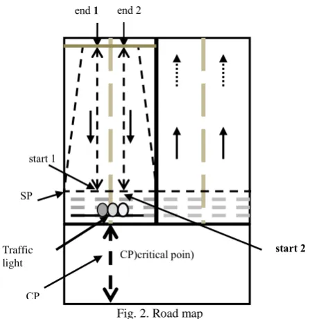
The length of the queue has been calculated in 6 ways (for street that has two lanes as shown in Fig. 2).

Fig. 2. Road map

The distance between two points of the XY-plane can be found using Eq. (10), which calculates the distance between (x1, y1) and (x2, y2) [13].

(10) )

( )

( 2 1 2

2 1

2 x y y

x

D   

Let the first column be Start1; the start of the second column be Start2; the end of the first column End1; the end of the second column End2; the start point of the street (SP); the beginning of the queue from SP is SR. The empty space between the queues is EL, and the safety zone CP. In this work, six cases is considered as queues categories, these are: Case 1:

End1<End2 && Start1>Start2

D=|End2-Start2| (11)

SR= |SP-End2| Case 2:

End1>End2 && Start1<Start2

D=|End1-Start1| (12)

SR=|SP-End1| Case 3:

Start2<End1 && End1<End2 && Start1<Start2

D=|End2-Start1| (13)

SR=|SP-End2| Case 4:

End1>End2 && Start1<End2 && Start1>Start2

D=|End1-Start2| (14)

SR=|SP-End1| Case 4:

End1<Start2

D=(End1-Start1)+(End2-Start2) (15)

EL=|Start2-End1|

SR=|SP-End2|

Case 6:

End2<Start1

D=(End1-Start1)+(End2-Start2) (16)

EL=|Start1-End2|

SR=|SP-End1|

After obtaining the queue length of the two lanes, the queue lengths are divided by the assumed car length to find the expected number of cares (NV) using Eq. (17). In this research, the average length of the car almost 100 pixel with respect to the used image resolution.

NV = Q_length/ 100 (17)

In Eq. (15) and (16), we know that there is space between queues. We need to calculate the distance and deduce the time needed by the vehicle to cross through. Fig. 3 shows the flow graph of the Queue Length Module.

Fig. 3. Queue length module

V. TIMING MODULE

The estimated time for each technique (depending on the computed number of vehicles) is calculated and compared with the actual time from control unit.

To find out the estimated time needed for green traffic light, the following factors should be calculated:

 Number of Vehicles (NV).

 The distance of the first vehicle from the Start Point (SR). The distance is set to one vehicle length. Since it is open area, it was given half the time needed for vehicle movement.

 The time needed to move to the next point is set to two seconds (MT).

 Distance between vehicles (EL) which represents empty levels. Estimated time for EL is one second.

( ni(i PaPitirc)PC

1

r

dCe dCer2

1 tat a

Traffic light

2 tsats

After calculating the above factors, the total number of vehicles (NV) that affect the estimated time is calculated using Eq. (17). The estimated time (in seconds) is calculated using Eq. (18).

Time =)NV×MT(+SR +EL (18)

VI.EXPERIMENTAL RESULTS

To evaluate the performance of the proposed approach, 32 images were taken with different sizes but with the same resolution. These images are partitioned into two datasets, according to the number of cars in the image. Crowd images (high density), and few cars with a lot of space (low density) as shown in Figs (A1, A2) in appendix A. Each of the two sets will be analyzed separately. The behavior of the suggested approach is evaluated by comparing the predicted number of cars (NV) compared with the actual number of cars in each picture. The actual time was calculated as follows (after dividing the road into levels as in Fig. 4):

Fig. 4. Image is Divided Into Levels

Let SV be number of small vehicles. Assume BV represents number of large vehicle. Each large vehicle is counted as two small vehicles.

1)

2)

3)

4)

5)

6)

Figs (5-8) show the comparison between the actual and the suggested vision based system. The comparison is from number of vehicle, and estimated time point of views (considering both low-density images and high density images).

Fig. 6. Number of Vehicle in Low Density

Fig. 7. Estimated Time High Density

Fig. 8. Number of Vehicle For High Density

Figs (5 and 6) show the estimated time and estimated number of vehicles in images with low densities. One could notice that the difference between estimated time and actual time is relatively high. Also, the difference between estimated number of vehicles and actual number of vehicles is relatively high. This is because counting vehicles in the queue is based on the deference between first and last vehicle divided by vehicle size, regardless if the vehicles exist or not.

Figs (7 and 8) show the estimated time and estimated number of vehicles in images with high densities. It is noticeable that the queuing system shows better performance with high density pictures.

affect the calculation of estimated time. Therefore, the error rate increases with low density roads, where vehicles are scattered.

VII.CONCLUSION

In this paper, vision based traffic control is developed. In the suggested approach, edge detection is used to find traffic queue length in 2 lane road. The estimated number of vehicles and the estimated time needed for green light period is calculated. From the experimental results, it was found that queue length approach needs approximately 11.0849 second (8.936 sec for preprocessing and 2.438 sec for queue algorithm) to make decision. From estimated-time and number-of-vehicles point of view, we concluded that the queue length is better for high density situations. To convert images to binary form, it was found that (by trial and error) the best threshold value is 20. Choosing proper threshold partially solves day light shadows problem. As future work, handling weather and night vision problem need to be solved.

REFERENCES

[1] Markos Papageoggius, Christina Diakaki, Vaya Dinopoulou, Apoatolos Kotsialos, and Yibing Wang, ―Review of Road Traffic Control Strategies‖, PROCEEDINGS OF THE IEEE, Vol. 91, No. 12, (2003).

[2] Hsu, W.L.; Liao, H.Y.M.; Jeng, B.S.; Fan, ―Real-time vehicle tracking on highway‖ The Proceedings of the IEEE International Conference on Intelligent Transportation Systems, Vol.2, pp. 909- 914 (2003).

[3] Haritaoglu, I., Harwood, D., Davis, L.S., "W4: real-time surveillance of people and their activities", Pattern Analysis and Machine Intelligence, IEEE Transactions, Vol. 22, Issue 8, pp. 809–830, (2000)

[4] Giusto, D.D., Massidda, F., Perra, C.,"A fast algorithm for video segmentation and object tracking", Digital signal Processing, 14th International Conference on, Vol. 2, pp. 697–700, (2002)

[5] Alvaro Soto and Aldo Cipriano , "Image processing applied to real time measurement of traffic flow" System Theory, Proceedings of the Twenty-Eighth Southeastern Symposium, IEEE Press, The Institute of Electrical and Electronics Engineers, Inc., pp. 312–316, (1996). [6] Y. L. Murphey, H. Lu, S. Lakshmanan, R. Karlsen, G. Gerhart, and T.

Meitzler, ―Dyta: An intelligent system for moving target detection,‖ in Proc. 10th _{Int. Conference of Image Analysis and}

Processing,Venice, Italy, pp. 1116–1121, (1999).

[7] Lawrence Y. Deng, Nick C. Tang, Dong-liang Lee, Chin Thin Wang and Ming Chih Lu, "Vision Based Adaptive Traffic Signal Control System development", Proceedings of the 19th _{International}

Conference on Advanced Information Networking and Applications (AINA’05), IEEE Press. (2005)

[8] Richard Lipka, Pavel Herout, "Implementation of Traffic Lights in JUTS", 10th _{International Conference on Computer Modeling and}

Simulation, Uksim, pp. 422-427, (2008).

[9] Choudekar, P., Banerjee, S., and Muju, M.K. ―Implementation of image processing in real time traffic light control‖. Electronics Computer Technology (ICECT), 3rd _{International Conference, IEEE}

Press, Vol. 2, pp. 94 – 98, (2011)

[10] Gonzalez, R. C. and Woods, R. E. "Digital image processing", 3rd

Ed., Prentice Hall, (2012).

[11] Mathworks website : http:// www.mathworks.com/

[12] Rebecca Vincent and Olusegun Folorunso,"A Descriptive Algorithm for Sobel Image Edge Detection", Proceedings of Informing Science & IT Education Conference (InSITE), (2009).

[13] Howard Anton, IrI Bivens, Stephen Davis, ―Calculus Early Transcendentals‖, 10th Edition, Wiley, (2012).

APPENDIXA

Figures A1 rHigh Density

Fig. A1. High density Images

Fig. A2. Low density Images