Applying Conditional Random Fields to Japanese Morphological Analysis

Applying Conditional Random Fields to Japanese Morphological Analysis

Taku Kudo†∗ Kaoru Yamamoto‡ Yuji Matsumoto†

†Nara Institute of Science and Technology 8916-5, Takayama-Cho Ikoma, Nara, 630-0192 Japan

‡CREST JST, Tokyo Institute of Technology 4259, Nagatuta Midori-Ku Yokohama, 226-8503 Japan

[email protected], [email protected], [email protected]

Abstract

This paper presents Japanese morphological analy-sis based on conditional random fields (CRFs). Pre-vious work in CRFs assumed that observation se-quence (word) boundaries were fixed. However, word boundaries are not clear in Japanese, and hence a straightforward application of CRFs is not possible. We show how CRFs can be applied to situations where word boundary ambiguity exists. CRFs offer a solution to the long-standing prob-lems in corpus-based or statistical Japanese mor-phological analysis. First, flexible feature designs for hierarchical tagsets become possible. Second, influences of label and length bias are minimized. We experiment CRFs on the standard testbed corpus used for Japanese morphological analysis, and eval-uate our results using the same experimental dataset as the HMMs and MEMMs previously reported in this task. Our results confirm that CRFs not only solve the long-standing problems but also improve the performance over HMMs and MEMMs.

1 Introduction

Conditional random fields (CRFs) (Lafferty et al., 2001) applied to sequential labeling problems are conditional models, trained to discriminate the cor-rect sequence from all other candidate sequences without making independence assumption for fea-tures. They are considered to be the state-of-the-art framework to date. Empirical successes with CRFs have been reported recently in part-of-speech tag-ging (Lafferty et al., 2001), shallow parsing (Sha and Pereira, 2003), named entity recognition (Mc-Callum and Li, 2003), Chinese word segmenta-tion (Peng et al., 2004), and Informasegmenta-tion Extracsegmenta-tion (Pinto et al., 2003; Peng and McCallum, 2004).

Previous applications with CRFs assumed that observation sequence (e.g. word) boundaries are fixed, and the main focus was to predict label

∗

At present, NTT Communication Science Laboratories, 2-4, Hikaridai, Seika-cho, Soraku, Kyoto, 619-0237 Japan [email protected]

sequence (e.g. part-of-speech). However, word boundaries are not clear in non-segmented lan-guages. One has to identify word segmentation as well as to predict part-of-speech in morphological analysis of non-segmented languages. In this pa-per, we show how CRFs can be applied to situations where word boundary ambiguity exists.

CRFs offer a solution to the problems in Japanese morphological analysis with hidden Markov models (HMMs) (e.g., (Asahara and Matsumoto, 2000)) or with maximum entropy Markov models (MEMMs) (e.g., (Uchimoto et al., 2001)). First, as HMMs are generative, it is hard to employ overlapping fea-tures stemmed from hierarchical tagsets and non-independent features of the inputs such as surround-ing words, word suffixes and character types. These features have usually been ignored in HMMs, de-spite their effectiveness in unknown word guessing. Second, as mentioned in the literature, MEMMs could evade neither from label bias (Lafferty et al., 2001) nor from length bias (a bias occurring because of word boundary ambiguity). Easy se-quences with low entropy are likely to be selected during decoding in MEMMs. The consequence is serious especially in Japanese morphological anal-ysis due to hierarchical tagsets as well as word boundary ambiguity. The key advantage of CRFs is their flexibility to include a variety of features while avoiding these bias.

In what follows, we describe our motivations of applying CRFs to Japanese morphological analysis (Section 2). Then, CRFs and their parameter esti-mation are provided (Section 3). Finally, we dis-cuss experimental results (Section 4) and give con-clusions with possible future directions (Section 5).

2 Japanese Morphological Analysis

2.1 Word Boundary Ambiguity

Input: “ ” (I live in Metropolis of Tokyo .)

BOS

(east)

[Noun]

(Tokyo)

[Noun]

(Kyoto)

[Noun]

(Metro.)

[Suffix]

(in)

[Particle]

(resemble)

[Verb]

(live)

[Verb]

EOS

Lattice:

(capital)

[Noun]

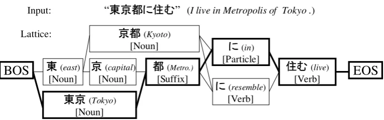
Figure 1: Example of lattice for Japanese morphological analysis

However, B/I tagging is not a standard method in 20-year history of corpus-based Japanese morpho-logical analysis. This is because B/I tagging cannot directly reflect lexicons which contain prior knowl-edge about word segmentation. We cannot ignore a lexicon since over 90% accuracy can be achieved even using the longest prefix matching with the lex-icon. Moreover, B/I tagging produces a number of redundant candidates which makes the decoding speed slower.

Traditionally in Japanese morphological analysis, we assume that a lexicon, which lists a pair of a word and its corresponding part-of-speech, is avail-able. The lexicon gives a tractable way to build a lattice from an input sentence. A lattice represents all candidate paths or all candidate sequences of to-kens, where each token denotes a word with its part-of-speech1.

Figure 1 shows an example where a total of 6 candidate paths are encoded and the optimal path is marked with bold type. As we see, the set of la-bels to predict and the set of states in the lattice are different, unlike English part-of-speech tagging that word boundary ambiguity does not exist.

Formally, the task of Japanese morphological analysis can be defined as follows. Let x be an input, unsegmented sentence. Let y be a path, a sequence of tokens where each token is a pair of word wi and its part-of-speechti. In other words,

y = (hw₁, t₁i, . . . ,hw_#y, t_#yi) where #y is the number of tokens in the pathy. LetY(x)be a set of candidate paths in a lattice built from the input sen-tencexand a lexicon. The goal is to select a correct path yˆ from all candidate paths in the Y(x). The distinct property of Japanese morphological analy-sis is that the number of tokensy varies, since the set of labels and the set of states are not the same.

1_{If one cannot build a lattice because no matching word can}

be found in the lexicon, unknown word processing is invoked. Here, candidate tokens are built using character types, such as

hiragana, katakana, Chinese characters, alphabets, and

num-bers.

2.2 Long-Standing Problems

2.2.1 Hierarchical Tagset

Japanese part-of-speech (POS) tagsets used in the two major Japanese morphological analyzers ChaSen2 _{and JUMAN}3 _{take the form of a}

hierar-chical structure. For example, IPA tagset4 used in ChaSen consists of three categories: part-of-speech, conjugation form (cform), and conjugate type (ctype). The cform and ctype are assigned only to words that conjugate, such as verbs and adjec-tives. The part-of-speech has at most four levels of subcategories. The top level has 15 different cate-gories, such as Noun, Verb, etc. Noun is subdivided into Common Noun, Proper Noun and so on. Proper Noun is again subdivided into Person, Organization or Place, etc. The bottom level can be thought as the word level (base form) with which we can com-pletely discriminate all words as different POS. If we distinguish each branch of the hierarchical tree as a different label (ignoring the word level), the to-tal number amounts to about 500, which is much larger than the typical English POS tagset such as Penn Treebank.

The major effort has been devoted how to in-terpolate each level of the hierarchical structure as well as to exploit atomic features such as word suf-fixes and character types. If we only use the bot-tom level, we suffer from the data sparseness prob-lem. On the other hand, if we use the top level, we lack in granularity of POS to capture fine dif-ferences. For instance, some suffixes (e.g., san or kun) appear after names, and are helpful to detect words with Name POS. In addition, the conjugation form (cfrom) must be distinguished appearing only in the succeeding position in a bi-gram, since it is dominated by the word appearing in the next.

Asahara et al. extended HMMs so as to incorpo-rate 1) position-wise grouping, 2) word-level

statis-2

http://chasen.naist.jp/

3_{http://www.kc.t.u-tokyo.ac.jp/nl-resource/juman.html} 4

tics, and 3) smoothing of word and POS level statis-tics (Asahara and Matsumoto, 2000). However, the proposed method failed to capture non-independent features such as suffixes and character types and se-lected smoothing parameters in an ad-hoc way.

2.2.2 Label Bias and Length Bias

It is known that maximum entropy Markov mod-els (MEMMs) (McCallum et al., 2000) or other dis-criminative models with independently trained next-state classifiers potentially suffer from the label bias (Lafferty et al., 2001) and length bias. In Japanese morphological analysis, they are extremely serious problems. This is because, as shown in Figure 1, the branching variance is considerably high, and the number of tokens varies according to the output path.

P(A, D | x) = 0.6 * 0.6 * 1.0 = 0.36 P(B | x) = 0.4 * 1.0 = 0.4

BOS

A

B

D

C

E

0.4

1.0 1.0

1.0

1.0 0.4

0.6 EOS

P(A, D | x) = 0.6 * 0.6 * 1.0 = 0.36 P(B, E | x) = 0.4 * 1.0 * 1.0 = 0.4

(a)

BOS

B

D

C

0.4 1.0

1.0

1.0 0.4

EOS

(b)

P(A,D|x) < P(B,E|x)

P(A,D|x) < P(B |x)

A

0.6

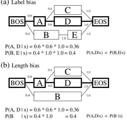
Figure 2: Label and length bias in a lattice

An example of the label bias is illus-trated in Figure 2:(a) where the path is searched by sequential combinations of maximum entropy models (MEMMs), i.e., P(y|x) = Q#_i=1y p(hwi, tii|hwi−1, ti−1i). Even

if MEMMs learn the correct path A-D with in-dependently trained maximum entropy models, the path B-E will have a higher probability and then be selected in decoding. This is because the token B has only the single outgoing token E, and the transition probability for B-E is always 1.0. Generally speaking, the complexities of transitions vary according to the tokens, and the transition probabilities with low-entropy will be estimated high in decoding. This problem occurs because the training is performed only using the correct path,

ignoring all other transitions.

Moreover, we cannot ignore the influence of the length bias either. By the length bias, we mean that short paths, consisting of a small number of tokens, are preferred to long path. Even if the transition probability of each token is small, the total proba-bility of the path will be amplified when the path is short 2:(b)). Length bias occurs in Japanese mor-phological analysis because the number of output tokensyvaries by use of prior lexicons.

Uchimoto et al. attempted a variant of MEMMs for Japanese morphological analysis with a number of features including suffixes and character types (Uchimoto et al., 2001; Uchimoto et al., 2002; Uchimoto et al., 2003). Although the performance of unknown words were improved, that of known words degraded due to the label and length bias. Wrong segmentation had been reported in sentences which are analyzed correctly by naive rule-based or HMMs-based analyzers.

3 Conditional Random Fields

Conditional random fields (CRFs) (Lafferty et al., 2001) overcome the problems described in Sec-tion 2.2. CRFs are discriminative models and can thus capture many correlated features of the inputs. This allows flexible feature designs for hierarchical tagsets. CRFs have a single exponential model for the joint probability of the entire paths given the in-put sentence, while MEMMs consist of a sequential combination of exponential models, each of which estimates a conditional probability of next tokens given the current state. This minimizes the influ-ences of the label and length bias.

As explained in Section 2.1, there is word bound-ary ambiguity in Japanese, and we choose to use a lattice instead of B/I tagging. This implies that the set of labels and the set of states are differ-ent, and the number of tokens #y varies accord-ing to a path. In order to accomodate this, we de-fine CRFs for Japanese morphological analysis as the conditional probability of an output path y =

(hw1, t1i, . . . ,hw#y, t#yi)given an input sequence x:

P(y|x) = 1

Zxexp

_X#y

i=1 X

k

λkfk(hwi−1, ti−1i,hwi, tii)

,

whereZxis a normalization factor over all

candi-date paths, i.e.,

Zx=

X

y0_∈Y(x)

exp

#y0

X

i=1 X

k

λkfk(hw0i−1, ti0−1i,hwi0, t0ii)

fk(hwi−1, ti−1i,hwi, tii)is an arbitrary feature func-tion overi-th tokenhwi, tii, and its previous token hwi−1, ti−1i5. λk(∈Λ={λ1, . . . , λK} ∈RK)is a learned weight or parameter associated with feature functionfk.

Note that our formulation of CRFs is different from the widely-used formulations (e.g., (Sha and Pereira, 2003; McCallum and Li, 2003; Peng et al., 2004; Pinto et al., 2003; Peng and McCallum, 2004)). The previous applications of CRFs assign a conditional probability for a label sequencey = y₁, . . . , y_T given an input sequencex=x1, . . . , xT as:

P(y|x) = 1

Zx exp

T X

i=1 X

k

λkfk(yi−1, yi,x)

In our formulation, CRFs deal with word boundary ambiguity. Thus, the the size of output sequenceT is not fixed through all candidatesy ∈ Y(x). The indexiis not tied with the inputxas in the original CRFs, but unique to the outputy∈ Y(x).

Here, we introduce the global feature vec-tor F(y,x) = {F1(y,x), . . . , FK(y,x)}, where F_k(y,x) = P#_i=1yf_k(hw_i−1, t_i−1i,hw_i, t_ii). Using the global feature vector, P(y|x) can also be rep-resented as P(y|x) = _Z1_xexp(Λ·F(y,x)). The most probable pathyˆfor the input sentencexis then given by

ˆ

y= argmax

y∈Y(x)

P(y|x) = argmax y∈Y(x)

Λ·F(y,x),

which can be found with the Viterbi algorithm. An interesting note is that the decoding process of CRFs can be reduced into a simple linear combina-tions over all global features.

3.1 Parameter Estimation

CRFs are trained using the standard maximum likelihood estimation, i.e., maximizing the log-likelihood LΛ of a given training set T =

{hx_j,y_ji}N j=1,

ˆ

Λ= argmax Λ∈RK

LΛ, where

LΛ =

X

j

log(P(yj|xj))

=X j

h

log X y∈Y(xj)

exp Λ·[F(yj,xj)−F(y,xj)] i

=X j

h

Λ·F(yj,xj)−log(Zxj) i

.

5

We could use trigram or more generaln-gram feature func-tions (e.g.,fk(hwi−n, ti−ni, . . . ,hwi, tii)), however we restrict ourselves to bi-gram features for clarity.

To maximize LΛ, we have to maximize the

dif-ference between the inner product (or score) of the correct path Λ ·F(yj,xj) and those of all other candidates Λ · F(y,xj), y ∈ Y(xj). CRFs is thus trained to discriminate the correct path from all other candidates, which reduces the influences of the label and length bias in encoding.

At the optimal point, the first-derivative of the log-likelihood becomes 0, thus,

δLΛ

δλk = X

j

Fk(yj,xj)−EP(y|xj)

Fk(y,xj)

= Ok−Ek= 0,

where Ok =

P

jFk(yj,xj) is the count of fea-ture_P k observed in the training data T, and Ek = jEP(y|xj)[Fk(y,xj)] is the expectation of fea-ture k over the model distribution P(y|x) and T. The expectation can efficiently be calculated using a variant of the forward-backward algorithm.

E_P(y|x)[F_k(y,x)] =

X

{hw0_,t0_{i,hw,ti}∈B(x)}

α_hw0_,t0_i·f_k∗·exp(

P

k0λk0f_k∗0)·β_hw,ti

Zx ,

wheref_k∗ is an abbreviation forfk(hw0, t0i,hw, ti), B(x) is a set of all bi-gram sequences observed in the lattice for x, and αhw,ti and βhw,ti are the forward-backward costs given by the following re-cursive definitions:

αhw,ti =

X

hw0_,t0_{i∈LT(hw,ti)}

αhw0_,t0_i·exp

X

k

λkfk(hw0, t0i,hw, ti)

βhw,ti =

X

hw0_,t0_{i∈RT(hw,ti)}

βhw0_,t0_i·exp

X

k

λkfk(hw, ti,hw0, t0i)

,

whereLT(hw, ti) andRT(hw, ti)denote a set of tokens each of which connects to the token hw, ti from the left and the right respectively. Note that initial costs of two virtual tokens, α_hwbos,tbosi and β_hweos,teosi, are set to be 1. A normalization constant is then given byZx=αhweos,teosi(=βhwbos,tbosi).

We attempt two types of regularizations in order to avoid overfitting. They are a Gaussian prior (L2-norm) (Chen and Rosenfeld, 1999) and a Laplacian prior (L1-norm) (Goodman, 2004; Peng and Mc-Callum, 2004)

LΛ=C

X

j

log(P(yj|xj))− 1 2

P

k|λk| (L1-norm) P

Below, we refer to CRFs with L1-norm and L2-norm regularization as L1-CRFs and L2-CRFs re-spectively. The parameter C ∈ R+ is a hyperpa-rameter of CRFs determined by a cross validation.

L1-CRFs can be reformulated into the con-strained optimization problem below by letting λk=λ+_k −λ−_k:

max : CX

j

log(P(yj|xj))− X

k (λ+

k +λ−k)/2

s.t., λ+

k ≥0, λ−k ≥0.

At the optimal point, the following Karush-Kuhun-Tucker conditions satisfy: λ+_k ·[C·(Ok −Ek)−

1/2] = 0, λ−_k ·[C ·(Ek −Ok)−1/2] = 0, and |C ·(O_k −E_k)| ≤ 1/2. These conditions mean that bothλ+_k andλ−_k are set to be 0 (i.e.,λk = 0), when |C·(Ok−Ek)| < 1/2. A non-zero weight is assigned to λk, only when |C ·(Ok −Ek)| =

1/2. L2-CRFs, in contrast, give the optimal solution when δLΛ

δλk =C·(Ok−Ek)−λk= 0. Omitting the proof,(Ok−Ek) 6= 0can be shown and L2-CRFs thus give a non-sparse solution where all λk have non-zero weights.

The relationship between two reguralizations have been studied in Machine Learning community. (Perkins et al., 2003) reported that L1-regularizer should be chosen for a problem where most of given features are irrelevant. On the other hand, L2-regularizer should be chosen when most of given features are relevant. An advantage of L1-based regularizer is that it often leads to sparse solutions where most of λk are exactly 0. The features as-signed zero weight are thought as irrelevant fea-tures to classifications. The L2-based regularizer, also seen in SVMs, produces a non-sparse solution where all ofλkhave non-zero weights. All features are used with L2-CRFs.

The optimal solutions of L2-CRFs can be ob-tained by using traditional iterative scaling algo-rithms (e.g., IIS or GIS (Pietra et al., 1997)) or more efficient quasi-Newton methods (e.g., L-BFGS (Liu and Nocedal, 1989)). For L1-CRFs, constrained op-timizers (e.g., L-BFGS-B (Byrd et al., 1995)) can be used.

4 Experiments and Discussion

4.1 Experimental Settings

We use two widely-used Japanese annotated cor-pora in the research community, Kyoto Univer-sity Corpus ver 2.0 (KC) and RWCP Text Corpus (RWCP), for our experiments on CRFs. Note that each corpus has a different POS tagset and details (e.g., size of training and test dataset) are summa-rized in Table 1.

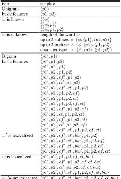
One of the advantages of CRFs is that they are flexible enough to capture many correlated fea-tures, including overlapping and non-independent features. We thus use as many features as possi-ble, which could not be used in HMMs. Table 2 summarizes the set of feature templates used in the

KC data. The templates for RWCP are essentially

the same as those of KC except for the maximum level of POS subcatgeories. Word-level templates are employed when the words are lexicalized, i.e., those that belong to particle, auxiliary verb, or suf-fix6. For an unknown word, length of the word, up to 2 suffixes/prefixes and character types are used as the features. We use all features observed in the lattice without any cut-off thresholds. Table 1 also includes the number of features in both data sets.

We evaluate performance with the standard F-score (Fβ=1) defined as follows:

Fβ=1 = 2·Recall·P recision Recall+P recision ,

where Recall = # of correct tokens # of tokens in test corpus

P recision = # of correct tokens # of tokens in system output.

In the evaluations of F-scores, three criteria of cor-rectness are used: seg: (only the word segmentation is evaluated), top: (word segmentation and the top level of POS are evaluated), and all: (all informa-tion is used for evaluainforma-tion).

The hyperparameters C for L1-CRFs and L2-CRFs are selected by cross-validation. Experiments are implemented in C++ and executed on Linux with XEON 2.8 GHz dual processors and 4.0 Gbyte of main memory.

4.2 Results

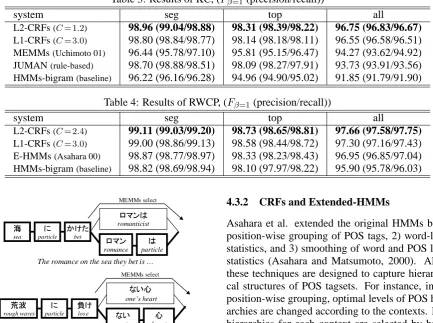
Tables 3 and 4 show experimental results using

KC and RWCP respectively. The three F-scores

(seg/top/all) for our CRFs and a baseline bi-gram HMMs are listed.

In Table 3 (KC data set), the results of a variant of maximum entropy Markov models (MEMMs) (Uchimoto et al., 2001) and a rule-based analyzer (JUMAN7) are also shown. To make a fare compar-ison, we use exactly the same data as (Uchimoto et al., 2001).

In Table 4 (RWCP data set), the result of an ex-tended Hidden Markov Models (E-HMMs)

(Asa-6_{These lexicalizations are usually employed in Japanese}

morphological analysis.

7

Table 1: Details of Data Set

KC RWCP

source Mainich News Article (’95) Mainich News Article (’94) lexicon (# of words) JUMAN ver. 3.61 (1,983,173) IPADIC ver. 2.7.0 (379,010) POS structure 2-levels POS, cfrom, ctype, base form 4-levels POS, cfrom, ctype, base form # of training sentences 7,958 (Articles on Jan. 1st - Jan. 8th) 10,000 (first 10,000 sentences)

# of training tokens 198,514 265,631

# of test sentences 1,246 (Articles on Jan. 9th) 25,743 (all remaining sentences)

# of test tokens 31,302 655,710

# of features 791,798 580,032

Table 2: Feature templates:fk(hw0, t0i,hw, ti) t0_=hp10_{, p2}0_{, cf}0_{, ct, bw}0_{i,t=hp1, p2, cf, ct, bwi, wherep1}0_/p1

andp20_{/p2are the top and sub categories of POS.cf}0_/cfandct0_/ct

are the cfrom and ctype respectively.bw0_{/bware the base form of the}

wordsw0_/w.

type template

Unigram hp1i basic features hp1, p2i wis known hbwi

hbw, p1i hbw, p1, p2i wis unknown length of the wordw

up to 2 suffixes× {φ,hp1i,hp1, p2i}

up to 2 prefixes× {φ,hp1i,hp1, p2i}

character type × {φ,hp1i,hp1, p2i} Bigram hp10_{, p1i}

basic features hp10_{, p1, p2i} hp10_{, p2}0_{, p1i} hp10_{, p2}0_{, p1, p2i} hp10_{, p2}0_{, cf}0_{, p1, p2i} hp10_{, p2}0_{, ct}0_{, p1, p2i} hp10_{, p2}0_{, cf}0_{, ct}0_{, p1, p2i} hp10_{, p2}0_{, p1, p2, cfi} hp10_{, p2}0_{, p1, p2, cti} hp10_{, p2}0_{, p1, p2, cf, cti} hp10_{, p2}0_{, cf}0_{, p1, p2, cfi} hp10_{, p2}0_{, ct, p1, p2, cti} hp10_{, p2}0_{, cf}0_{, p1, p2, cti} hp10_{, p2}0_{, ct}0_{, p1, p2, cfi} hp10_{, p2}0_{, cf}0_{, ct}0_{, p1, p2, cf, cti} w0

is lexicalized hp10_{, p2}0_{, cf}0_{, ct}0_{, bw}0_{, p1, p2i} hp10_{, p2}0_{, cf}0_{, ct}0_{, bw}0_{, p1, p2, cfi} hp10_{, p2}0_{, cf}0_{, ct}0_{, bw}0_{, p1, p2, cti} hp10_{, p2}0_{, cf}0_{, ct}0_{, bw}0_{, p1, p2, cf, cti} wis lexicalized hp10_{, p2}0_{, p1, p2, cf, ct, bwi}

hp10_{, p2}0_{, cf}0_{, p1, p2, cf, ct, bwi} hp10_{, p2}0_{, ct}0_{, p1, p2, cf, ct, bwi} hp10_{, p2}0_{, cf}0_{, ct}0_{, p1, p2, cf, ct, bwi} w0_{/ware lexicalized hp1}0_{, p2}0_{, cf}0_{, ct}0_{, bw}0_{, p1, p2, cf, ct, bwi}

hara and Matsumoto, 2000) trained and tested with the same corpus is also shown. E-HMMs is applied to the current implementation of ChaSen. Details of E-HMMs are described in Section 4.3.2.

We directly evaluated the difference of these sys-tems using McNemar’s test. Since there are no standard methods to evaluate the significance of F scores, we convert the outputs into the

character-based B/I labels and then employ a McNemar’s paired test on the labeling disagreements. This eval-uation was also used in (Sha and Pereira, 2003). The results of McNemar’s test suggest that L2-CRFs is significantly better than other systems including L1-CRFs8. The overall results support our empirical success of morphological analysis based on CRFs.

4.3 Discussion

4.3.1 CRFs and MEMMs

Uchimoto el al. proposed a variant of MEMMs trained with a number of features (Uchimoto et al., 2001). Although they improved the accuracy for un-known words, they fail to segment some sentences which are correctly segmented with HMMs or rule-based analyzers.

Figure 3 illustrates the sentences which are inrectly segmented by Uchimoto’s MEMMs. The cor-rect paths are indicated by bold boxes. Uchimoto et al. concluded that these errors were caused by non-standard entries in the lexicon. In Figure 3, “ロマ ンは” (romanticist) and “ない心” (one’s heart) are unusual spellings and they are normally written as “ロマン派” and “内心” respectively. However, we conjecture that these errors are caused by the influ-ence of the length bias. To support our claim, these sentences are correctly segmented by CRFs, HMMs and rule-based analyzers using the same lexicon as (Uchimoto et al., 2001). By the length bias, short paths are preferred to long paths. Thus, single to-ken “ロマンは” or “ない心” is likely to be selected compared to multiple tokens “ロマン /は” or “な

い/心”. Moreover, “ロマン” and “ロマンは” have exactly the same POS (Noun), and transition proba-bilities of these tokens become almost equal. Con-sequentially, there is no choice but to select a short path (single token) in order to maximize the whole sentence probability.

Table 5 summarizes the number of errors in HMMs, CRFs and MEMMs, using the KC data set. Two types of errors, l-error and s-error, are given in

8

In all cases, the p-values are less than1.0×10−4

Table 3: Results of KC, (Fβ=1(precision/recall))

system seg top all

L2-CRFs(C= 1.2) 98.96 (99.04/98.88) 98.31 (98.39/98.22) 96.75 (96.83/96.67)

L1-CRFs(C= 3.0) 98.80 (98.84/98.77) 98.14 (98.18/98.11) 96.55 (96.58/96.51) MEMMs(Uchimoto 01) 96.44 (95.78/97.10) 95.81 (95.15/96.47) 94.27 (93.62/94.92) JUMAN(rule-based) 98.70 (98.88/98.51) 98.09 (98.27/97.91) 93.73 (93.91/93.56) HMMs-bigram(baseline) 96.22 (96.16/96.28) 94.96 (94.90/95.02) 91.85 (91.79/91.90)

Table 4: Results of RWCP, (Fβ=1(precision/recall))

system seg top all

L2-CRFs(C= 2.4) 99.11 (99.03/99.20) 98.73 (98.65/98.81) 97.66 (97.58/97.75)

L1-CRFs(C= 3.0) 99.00 (98.86/99.13) 98.58 (98.44/98.72) 97.30 (97.16/97.43) E-HMMs(Asahara 00) 98.87 (98.77/98.97) 98.33 (98.23/98.43) 96.95 (96.85/97.04) HMMs-bigram(baseline) 98.82 (98.69/98.94) 98.10 (97.97/98.22) 95.90 (95.78/96.03)

sea

particle

bet

romanticist

romance

particle

The romance on the sea they bet is …

rough waves

particle

los e not

heart

one’s heart

A heart which beats rough waves is … MEMMs select MEMMs select

Figure 3: Errors with MEMMs (Correct paths are marked with bold boxes.)

Table 5: Number of errors in KC dataset # of l-errors # of s-errors

CRFs 79 (40%) 120 (60%)

HMMs 306 (44%) 387 (56%)

MEMMs 416 (70%) 183 (30%)

l-error: output longer token than correct one s-error: output shorter token than correct one

this table. l-error (or s-error) means that a system incorrectly outputs a longer (or shorter) token than the correct token respectively. By length bias, long tokens are preferred to short tokens. Thus, larger number of l-errors implies that the result is highly influenced by the length bias.

While the relative rates of l-error and s-error are almost the same in HMMs and CRFs, the number of l-errors with MEMMs amounts to 416, which is 70% of total errors, and is even larger than that of naive HMMs (306). This result supports our claim that MEMMs is not sufficient to be applied to Japanese morphological analysis where the length bias is inevitable.

4.3.2 CRFs and Extended-HMMs

Asahara et al. extended the original HMMs by 1) position-wise grouping of POS tags, 2) word-level statistics, and 3) smoothing of word and POS level statistics (Asahara and Matsumoto, 2000). All of these techniques are designed to capture hierarchi-cal structures of POS tagsets. For instance, in the position-wise grouping, optimal levels of POS hier-archies are changed according to the contexts. Best hierarchies for each context are selected by hand-crafted rules or automatic error-driven procedures.

CRFs can realize such extensions naturally and straightforwardly. In CRFs, position-wise grouping and word-POS smoothing are simply integrated into a design of feature functions. Parameters λk for each feature are automatically configured by gen-eral maximum likelihood estimation. As shown in Table 2, we can employ a number of templates to capture POS hierarchies. Furthermore, some over-lapping features (e.g., forms and types of conjuga-tion) can be used, which was not possible in the ex-tended HMMs.

4.3.3 L1-CRFs and L2-CRFs

5 Conclusions and Future Work

In this paper, we present how conditional random fields can be applied to Japanese morphological analysis in which word boundary ambiguity exists. By virtue of CRFs, 1) a number of correlated fea-tures for hierarchical tagsets can be incorporated which was not possible in HMMs, and 2) influences of label and length bias are minimized which caused errors in MEMMs. We compare results between CRFs, MEMMs and HMMs in two Japanese anno-tated corpora, and CRFs outperform the other ap-proaches. Although we discuss Japanese morpho-logical analysis, the proposed approach can be ap-plicable to other non-segmented languages such as Chinese or Thai.

There exist some phenomena which cannot be an-alyzed only with bi-gram features in Japanese mor-phological analysis. To improve accuracy, tri-gram or more general n-gram features would be useful. CRFs have capability of handling such features. However, the numbers of features and nodes in the lattice increase exponentially as longer contexts are captured. To deal with longer contexts, we need a practical feature selection which effectively trades between accuracy and efficiency. For this challenge, McCallum proposes an interesting research avenue to explore (McCallum, 2003).

Acknowledgments

We would like to thank Kiyotaka Uchimoto and Masayuki Asahara, who explained the details of their Japanese morphological analyzers.

References

Masayuki Asahara and Yuji Matsumoto. 2000. Ex-tended models and tools for high-performance part-of-speech tagger. In Proc of COLING, pages 21–27.

Richard H. Byrd, Peihuang Lu, Jorge Nocedal, and Ci You Zhu. 1995. A limited memory algorithm for bound constrained optimization. SIAM Jour-nal on Scientific Computing, 16(6):1190–1208. Stanley F. Chen and Ronald. Rosenfeld. 1999. A

gaussian prior for smoothing maximum entropy models. Technical report, Carnegie Mellon Uni-versity.

Joshua Goodman. 2004. Exponential priors for maximum entropy models. In Proc. of HLT/NAACL.

John Lafferty, Andrew McCallum, and Fernando Pereira. 2001. Conditional random fields: Prob-abilistic models for segmenting and labeling se-quence data. In Proc. of ICML, pages 282–289.

Dong C. Liu and Jorge Nocedal. 1989. On the limited memory BFGS method for large scale optimization. Math. Programming, 45(3, (Ser. B)):503–528.

Andrew McCallum and Wei Li. 2003. Early re-sults for named entity recognition with condi-tional random fields, feature induction and web-enhanced lexicons. In In Proc. of CoNLL. Andrew McCallum, Dayne Freitag, and Fernando

Pereira. 2000. Maximum entropy markov mod-els for information and segmentation. In Proc. of ICML, pages 591–598.

Andrew McCallum. 2003. Efficiently inducing fea-tures of conditional random fields. In Nineteenth Conference on Uncertainty in Artificial Intelli-gence (UAI03).

Fuchun Peng and Andrew McCallum. 2004. Accu-rate information extraction from research papers. In Proc. of HLT/NAACL.

Fuchun Peng, Fangfang Feng, and Andrew McCal-lum. 2004. Chinese segmentation and new word detection using conditional random fields (to ap-pear). In Proc. of COLING.

Simon Perkins, Kevin Lacker, and James Thiler. 2003. Grafting: Fast, incremental feature selec-tion by gradient descent in funcselec-tion space. JMLR, 3:1333–1356.

Della Pietra, Stephen, Vincent J. Della Pietra, and John D. Lafferty. 1997. Inducing features of ran-dom fields. IEEE Transactions on Pattern Analy-sis and Machine Intelligence, 19(4):380–393. David Pinto, Andrew McCallum, Xing Wei, and

W. Bruce Croft. 2003. Table extraction using conditional random fields. In In Proc. of SIGIR, pages 235–242.

Fei Sha and Fernando Pereira. 2003. Shallow pars-ing with conditional random fields. In Proc. of HLT-NAACL, pages 213–220.

Kiyotaka Uchimoto, Satoshi Sekine, and Hitoshi Isahara. 2001. The unknown word problem: a morphological analysis of Japanese using maxi-mum entropy aided by a dictionary. In Proc. of EMNLP, pages 91–99.

Kiyotaka Uchimoto, Chikashi Nobata, Atsushi Yamada, Satoshi Sekine, and Hitoshi Isahara. 2002. Morphological analysis of the spontaneous speech corpus. In Proc of COLING, pages 1298– 1302.