Empirical Likelihood Block Bootstrapping

(1)

Title

Author(s)

Allen, Jason; Gregory, Allan W.; Shimotsu, Katsumi

Citation

Issue Date

2010-03

Type

Technical Report

Text Version

publisher

URL

http://hdl.handle.net/10086/18323

(2)

Discussion Paper #2010–01

EMPIRICAL LIKELIHOOD BLOCK BOOTSTRAPPING

Jason Allen†, Allan W. Gregory‡, and Katsumi Shimotsu‡[∗

Financial Stability Department, Bank of Canada† Department of Economics, Queen’s University‡ Department of Economics, Hitotsubashi University[

March 13, 2010

Abstract

Monte Carlo evidence has made it clear that asymptotic tests based on generalized method of moments (GMM) estimation have disappointing size. The problem is exacerbated when the moment conditions are serially correlated. Several block bootstrap techniques have been proposed to correct the problem, including Hall and Horowitz (1996) and Inoue and Shintani (2006). We propose an empirical likelihood block bootstrap procedure to improve inference where models are characterized by nonlinear moment conditions that are serially correlated of possibly infinite order. Combining the ideas of Kitamura (1997) and Brown and Newey (2002), the parameters of a model are initially estimated by GMM which are then used to compute the empirical likelihood probability weights of the blocks of moment conditions. The probability weights serve as the multinomial distribution used in resampling. The first-order asymptotic validity of the proposed procedure is proven, and a series of Monte Carlo experiments show it may improve test sizes over conventional block bootstrapping.

Keywords: generalized methods of moments, empirical likelihood, block bootstrap

JEL classification: C14, C22

∗_{Correspondence can be sent to J. Allen ([email protected]). We thank Don Andrews, Geoffrey Dunbar,} Atushi Inoue, Gregor Smith, Silvia Gonc¸alves, Sharon Kozicki, Thanasis Stengos, and Tim Vogelsang for helpful com-ments and insightful discussion. We also thank seminar participants at the Bank of Canada, Indiana University, Queen’s University, Econometric Society World Congress in London (2005), Canadian Econometric Study Group in Vancouver (2005), and Far East Meetings of the Econometric Society in Taiwan (2007). We also thank the referee for insightful com-ments. We acknowledge the Social Sciences and Humanities Research Council of Canada for support of this research. The views in this paper do not necessarily reflect those of the Bank of Canada. All errors are our own.

(3)

1 Introduction

Generalized method of moments (GMM, Hansen (1982)) has been an essential tool for econo-metricians, partly because of its straightforward application and fairly weak restrictions on the data generating process. GMM estimation is widely used in applied economics to estimate and test as-set pricing models (Hansen and Singleton (1982), Kocherlakota (1990), Altonji and Segal (1996)), business cycle models (Christiano and Haan (1996)), models that use longitudinal data (Arellano and Bond (1991), Ahn and Schmidt (1995)), as well as stochastic dynamic general equilibrium models (Ruge-Murcia (2007)).

Despite the widespread use of GMM, there is ample evidence that the finite sample properties for inference have been disappointing (e.g. the 1996 special issue of JBES); t-tests on parameters and Hansen’s test of overidentifying restrictions (J-test, or Sargan test) for model specification perform poorly and tend to be biased away from the null hypothesis. The situation is especially severe for dependent data (see Clark (1996)). Consequently, inferences based on asymptotic critical values can often be very misleading. From an applied perspective, this means that theoretical models may be more frequently rejected than necessary due to poor inference rather than poor modeling.

Various attempts have been made to address finite sample size problems while allowing for de-pendence in the data. Berkowitz and Kilian (2000), Ruiz and Pascual (2002), and H¨ardle, Horowitz, and Kreiss (2003) review some of the techniques developed for bootstrapping time-series models, including financial time series. Lahiri (2003) is an excellent monograph on resampling methods for dependent data. Hall and Horowitz (1996) apply the block bootstrap approach to GMM and es-tablish the asymptotic refinements of their procedure when the moment conditions are uncorrelated after finitely many lags. Andrews (2002) provides similar results for thek-step bootstrap procedure first proposed by Davidson and Mackinnon (1999).

Limited Monte Carlo results indicate the block-bootstrap has some success at improving in-ference in GMM. More recent papers by Zvingelis (2003) and Inoue and Shintani (2006) attempt refinements to Hall and Horowitz (1996) and Andrews (2002). The main requirement of these ear-lier papers is that the data is serially uncorrelated after a finite number of lags. In contrast, Inoue and Shintani (2006) prove that the block bootstrap provides asymptotic refinements for the GMM estimator of linear models when the moment conditions are serially correlated of possibly infinite order. Zvingelis (2003) derives the optimal block length for coverage probabilities of normalized and Studentized statistics.

A complementary line of research has examined empirical likelihood (EL) estimators, or their generalization (GEL). Rather than try to improve the finite properties of the GMM estimator

(4)

di-rectly, researchers such as Kitamura (1997), Kitamura and Stutzer (1997), Smith (1997), and Im-bens, Spady, and Johnson (1998) have proposed and/or tested new statistics, ones based on GEL-estimators.1 _{A GEL estimator minimizes the distance between the empirical density and a synthetic}

density subject to the restriction that all the moment conditions are satisfied. GEL estimators have the same first-order asymptotic properties as GMM but have smaller bias than GMM in finite sam-ples. Furthermore, these biases do not increase in the number of overidentifying restrictions in the case of GEL. Newey and Smith (2004) provide theoretical evidence of the higher-order efficiency of GEL estimators. Gregory, Lamarche, and Smith (2002) have shown, however, that these alternatives to GMM do not solve the over-rejection problem in finite samples.

Brown and Newey (2002) introduce the empirical likelihood bootstrap technique foriid data. Rather than resampling from the empirical distribution function, the empirical likelihood bootstrap resamples from a multinomial distribution function, where the probability weights are computed by empirical likelihood. Brown and Newey (2002) show that empirical likelihood bootstrap provides an asymptotically efficient estimator of the distribution oftratios and overidentification test-statistics. The author’s Monte Carlo design features a dynamic panel model with persistence andiid error structure. The results suggest that the empirical likelihood bootstrap is more accurate than the asymptotic approximation, and not dissimilar to the Hall and Horowitz (1996) bootstrap.

In this paper, the approach of Brown and Newey (2002) is extended to the case of dependent data, using the empirical likelihood (Owen (1990)). A number of researchers have implemented this approach with some success in linear time-series models (Ramalho (2006)) as well as dynamic panel data models (Gonzalez (2007)). With serially correlated data the idea is that parameters of a model are initially estimated by GMM and then used to compute the empirical likelihood proba-bility weights of theblocksof moment conditions, which serve as the multinomial distribution for resampling. In this paper the first-order asymptotic validity of the proposed empirical likelihood block bootstrap is proven using the results in Gonc¸alves and White (2004) and the approach of Ma-son and Newton (1992), who analyze the consistency of generalized bootstrap (weighted bootstrap) procedures. Our consistency results may be viewed as an extension of Mason and Newton (1992) to block bootstrapping. We report on the finite-sample properties of t-ratios and overidentification test-statistics. A series of Monte Carlo experiments show that the empirical likelihood block bootstrap can reduce size distortions considerably and improve test sizes over first-order asymptotic theory and frequently outperforms conventional block bootstrapping approaches.2_{Furthermore, the}

empir-1_{See Kitamura (2007) for a review of recent research on empirical likelihood methods.}

2_{In addition to bootstrapping using empirical likelihood estimated weights it would seem natural to consider} subsam-pling using the same weights. Subsamsubsam-pling (Politis and Romano (1994), Politis, Romano, and Wolf (1999), and Hong and Scaillet (2006)) is an alternative to bootstrapping where each block is treated as it’s own series and test-statistics are calculated for each sub-series. This is left as future work.

(5)

ical likelihood block bootstrap does not require solving the difficult saddle point problem associated with GEL estimators. This is because estimation of the probability weights can be conducted by plugging-in first-stage GMM estimates. Difficulties with solving the saddle point problem is a com-mon argument acom-mongst applied researchers for not switching from GMM to EL, even though the latter is higher-order efficient.

In related work, Hall and Horowitz (1996) analyze an application of the block bootstrap to GMM. Hall and Horowitz (1996) assume that the moment conditions are uncorrelated after finitely many lags, and derive the higher-order improvements of the block bootstrap. The key insight of Hall and Horowitz (1996) is that, when the number of moment conditions exceeds the number of parameters, one needs to re-center the moment conditions because there is in general no parameter value such that the resampled moment conditions will be exactly equal to zero in expectation. One difference between our paper and Hall and Horowitz (1996) is that we do not assume that the moment conditions are uncorrelated after finitely many lags. Further, in the empirical likelihood block bootstrap one does not need to re-center the moment conditions by virtue of the EL weights. However, we only derive the consistency of our proposed procedure, and do not derive its higher-order properties.

The paper is organized as follows. Section 2 provides an overview of GMM and EL. Section 3 presents a discussion of how resampling methods might improve inference in GMM. Section 4 presents the asymptotic results. Section 5 presents the Monte Carlo design for both linear and nonlinear models. Section 6 concludes. The technical assumption and proofs are collected at the end of the paper in the mathematical appendix.

2 Overview of GMM and GEL

In this section we present an overview of GMM and EL to establish notation and framework.

2.1 GMM

LetXt∈Rk,t=1, . . .n, be a set of observations from a stochastic sequence. Suppose for some

true parameter valueθ₀(p×1) the following moment conditions (mequations) hold andp≤m<n:

(6)

whereg:Rk×Θ→Rm. The GMM estimator is defined as: ˆ θ=arg minQn(θ), Qn(θ) = Ã n−1 n

∑

t=1 g(Xt,θ) !₀ Wn Ã n−1 n

∑

t=1 g(Xt,θ) ! , (2) where the weighting matrixWn→pW. Hansen (1982) shows that the GMM estimator ˆθis consistent

and asymptotically normally distributed subject to some regularity conditions. The elements of

{g(Xt,θ)}and{∇g(x,θ)}are assumed to be near epoch dependent (NED) on theα-mixing sequence {V_t}of size−1 uniformly on(Θ,ρ)whereρis any convenient norm onRp_.

DefineΣ=limn→∞var(n−1/2∑nt=1g(Xt,θ0)). The standard kernel estimate ofΣis:

Sn(θ) = n

∑

h=−n k µ h m ¶ ˆ Γ(h,θ), (3)

wherek(·)is a kernel and ˆΓ(h,θ) =n−1∑n_t=h+₁g(Xt,θ)g(Xt+h,θ)0forh≥0 andn−1∑tn−h=1g(Xt,θ)g(Xt−h,θ)0

forh<0. It is known thatSn(θ˜)→pΣif ˜θ→pθ0under weak conditions on the kernel and

band-width; see de Jong and Davidson (2000).

The optimal weighting matrix is given bySn(θ˜)−1with ˜θ→pθ0. When the optimal weighting

matrix is used, the asymptotic covariance matrix of ˆθis(G0_Σ−1_G₎−1_{, where}_G₌_lim

n→∞E(n−1∑nt=1∇g(Xt,θ0))

with∇g(x,θ) =∂g(x,θ)/∂θ0_.

In terms of testing for model misspecification, the most popular test is Hansen’s J-test for overi-dentifying restrictions:

J

n=Kn(θˆn)0Kn(θˆn)→dχm−r, (4) where Kn(θ) =Sn−1/2n−1/2 n

∑

t=1 g(Xt,θ),

andSn is a consistent estimate ofΣ. Letθrdenote the rth element ofθ, and letθ0rdenote therth

element ofθ0. The t-statistic for testing the null hypothesisH0:θr=θ0ris:

Tnr= √

n(θˆnr−θ0r)

ˆ

σnr →dN(0,1), (5)

(7)

2.2 Empirical Likelihood

Empirical Likelihood (EL) estimation has some history in the statistical literature but has only recently been explored by econometricians. One attractive feature is that while its first-order asymp-totic properties are the same as GMM, there is an improvement for EL at the second-order (see Qin and Lawless (1994) and Newey and Smith (2004)). For time-series models see Anatolyev (2005). This suggests that there might be some gain for EL over GMM in finite sample performance. At present, limited Monte Carlo evidence (see Gregory, Lamarche, and Smith (2002)) has provided mixed results.

The idea of EL is to use likelihood methods for model estimation and inference without having to choose a specific parametric family or probability densities. The parameters are estimated by minimizing the distance between the empirical density and a density that identically satisfies all of the moment conditions. The main advantages over GMM are that it is invariant to linear transforma-tions of the moment functransforma-tions and does not require the calculation of the optimal weighting matrix for asymptotic efficiency (although smoothing or blocking of the moment condition is necessary for dependent data). The main disadvantage is that it is computationally more demanding than GMM in that a saddle point problem needs to be solved.

The Generalized Empirical Likelihood Estimator solves the following Lagrangian: maxL=1 n n

∑

t=1 h(·)−µ( n

∑

t=1 πt−1)−γ0 n

∑

t=1 πtg(xt,θ). (6)

Solving forπt gives

π_t = h1(δ0g(xt,θ))

∑h1(δ0g(xt,θ))

, h₁(v) =∂h(v)/∂v. (7)

In the case of EL,h(·) =log(πt). The presence of serially correlated observations necessitates a

modification of equation (6). Kitamura and Stutzer (1997) address the data dependency problem by smoothing the moment conditions. Anatolyev (2005) provides conditions on the amount of smoothing necessary for the bias of the GEL estimator to be less than the GMM estimator. Kitamura (1997) and Bravo (2005) address serial correlation in the moment conditions by using averages across blocks of data.

3 Improving Inference: Resampling Methods

This section presents an overview of block bootstrap methods typically used to improve infer-ence in models estimated by GMM and follows up with a detailed proposal of a new method based

(8)

on empirical likelihood.

3.1 The Block Bootstrap

The bootstrap amounts to treating the estimation data as if they were the population and gen-erating bootstrap observations by resampling the estimation data. If the estimation data is serially correlated, then blocks of data are resampled and the blocks are treated as theiidsample.

We implement two forms of the block bootstrap. The first approach implements the overlapping bootstrap (MBB, K¨unsch (1989)). Letbbe the number of blocks and`the block length, such that

n=b`. Theith overlapping block is ˜Xi={Xi, ...,Xi+`−1},i=1, ...,n−`+1. The MBB resample

is{X∗

t }nt=1={X˜1∗, ...,X˜b∗}, where ˜Xi∗∼iid(X˜1, ...,X˜n−`+1). The GMM estimator is therefore:

θ∗∗_MBB=arg minQ∗∗_MBB_,_n(θ), Q∗∗ MBB,n(θ) = ¡ n−1_∑n t=1g∗(Xt∗,θ) ¢₀ W∗∗ n ¡ n−1_∑n t=1g∗(Xt∗,θ) ¢ , whereg∗₍_X∗

t ,θ) =g(Xt∗,θ)−n−1∑nt=1g(Xt,θˆn) andWn∗∗ is a weighting matrix. That is, given a

weighting matrix W∗∗

n , the GMM estimator that minimizes the quadratic form of the demeaned

block-resampled moment conditions isθ∗∗ MBB.

Hall and Horowitz (1996) implement the nonoverlapping block bootstrap (NBB, Carlstein (1986)). This approach is also considered (in addition to the MBB). Letbbe the number of blocks and`the block length, and assumeb`=n. We resamplebblocks with replacement from{X˜_i:i=1, . . . ,b}

where ˜Xi= (X(i−1)`+1, . . . ,X(i−1)`+`). The NBB resample is{Xt∗}nt=1. The NBB version of the GMM

problem is identical to the MBB version, except for the way one resamples the data. We consider both MBB and NBB approaches because there is little known about the superiority of either method in finite samples.3

As shown in Gonc¸alves and White (2004) (hereafter GW04), because the resampledbblocks are (conditionally)iid, the bootstrap version of the long-run autocovariance matrix estimate takes the form (cf. equation (3.1) of GW04):

S∗∗_n (θ∗∗) =`b−1

∑

b i=1 Ã `−1

∑

` t=1 g∗(X_(i−∗ ₁₎_`_+t,θ∗∗) ! Ã `−1

∑

` t=1 g∗(X_(i−∗ ₁₎_`_+t,θ∗∗) !₀ , (8) whereθ∗∗ _{denotes either}_θ∗∗

MBB orθ∗∗NBB. The optimal weighting matrix is given by(Sn∗∗(θ˜∗∗))−1,

where ˜θ∗∗is the first-stage MBB/NBB estimator. The bootstrap version of the J-statistic,

J

∗∗ MBB,nand 3_{It is only known that the MBB is more efficient than the NBB in estimating the variance (Lahiri (1999)).}

(9)

J

∗∗

NBB,n, is defined analogously to

J

nbut using(Sn∗∗(θ˜∗∗))−1/2andn−1/2∑nt=1g∗(Xt∗,θ).

Note that in Hall and Horowitz (1996), the recentering of the sample moment condition is nec-essary in order to establish the asymptotic refinements of the bootstrap. This is because in general there is no θsuch that E∗_g₍_x_,_θ_{) =}_{0 when there are more moments than parameters and the}

re-sampling schemes must impose the null hypothesis. Recentering is not necessary for establishing the first-order validity of the bootstrap version of ˆθn (see Hahn (1996)), but is necessary for the

first-order validity of the bootstrap J-test.

Operationally one needs to choose a block size when implementing the block-bootstrap. H¨ardle, Horowitz, and Kreiss (2003) point out that the optimal block length depends on the objective of bootstrapping. That is, the block length depends on whether or not one is interested in bootstrapping one-sided or two-sided tests or whether one is concerned with estimating a distribution function. Among others, Zvingelis (2003) solves for optimal block lengths given different scenarios. Prac-tically, the optimal block lengths for each different hypothesis test are unlikely to be implemented since practitioner’s are interested in a variety of problems across various hypotheses. Experimenta-tion is done with fixed block lengths as well as data-dependent methods.

Following the literature we recommend using a data-dependent approach for selecting a block length. We set the block length equal to the data-driven lag length for the Bartlett kernel using the method proposed by Newey and West (1994). This is motivated by the asymptotic equivalence of the bootstrap variance to a Bartlett kernel variance estimator (see Bühlmann and Künsch (1999), equation (2.5)). Gonçalves and White (2004) use the automatic bandwidth selection procedure proposed by Andrews (1991) in their simulation study for similar reasons. There may be some gain in using a more advanced algorithm than the one we currently employ but given its simplicity and availability in pre-packaged GMM software, we believe that most practitioners are likely to continue using a Newey-West type lag-selection procedure.4 _{A number of approaches that are particular to}

block bootstrapping, but under different conditions than our model, have been suggested. Berkowitz and Kilian (2000) propose a two-step parametric approach for linear models and Politis and White (2004) propose an automatic block-length selection procedure based on spectral estimation (Politis and Romano (1995)), and which is appropriate for the circular and stationary bootstrap (Politis and Romano (1994)).

4_{Note that in the case of covariance matrix estimation there is also the issue of smoothing, and therefore the choice} of the appropriate kernel. The block samples in our approach, however, are (conditionally)iid, therefore the choice of kernel does not arise.

(10)

3.2 Empirical Likelihood Bootstrap

In this section we develop the empirical likelihood (EL) approach to bootstrapping time-series models. Two cases are considered: (i) the overlapping empirical likelihood block bootstrap (EMB), and (ii) the non-overlapping empirical likelihood block bootstrap (ENB). The procedure for imple-menting the empirical block bootstrap is straightforward and outlined in Section 7.

An advantage of the EL block bootstrap over the standard block bootstrap is that EL weighted observations estimate the distribution function of the data more efficiently than non-weighted obser-vations. We think this provides the EL block bootstrap with an improvement in test level accuracy over the standard block bootstrap, although a rigorous proof by an Edgeworth expansion is beyond the scope of the paper.

WhenX_t isiid, Theorem 1 of Brown and Newey (2002) shows that the empirical distribution function of the EL-weightedXt’s is a more efficient estimator of the population distribution function

ofXtthan the ordinary empirical distribution function of theXt’s. Brown and Newey (2002) combine

it with an Edgeworth expansion to show that the EL bootstrap improves test level accuracy over an

iidbootstrap for some cases, for example in a one-sided test of the null hypothesis ofE[g(Xt,θ0)] =

0.

In our case, we attach the EL weights to the blocks, instead of individual observations. By anal-ogy to Brown and Newey (2002), using the EL weights would provide a more efficient estimate of the distribution function of the blocks. Therefore, the EL block bootstrap would estimate the dis-tribution of the sample moments more efficiently than the standard block bootstrap. Our simulation results suggest that efficient estimation of the distribution of the blocks by the EL block bootstrap contributes to improvements in test level accuracy, at least in some cases.

On the other hand, it is not clear whether an Edgeworth-expansion based analysis can demon-strate a higher-order improvement of the EL block bootstrap over the first-order asymptotics. Inoue and Shintani (2006) demonstrate that a higher-order analysis of the block bootstrap is handicapped by the bias of the HAC covariance matrix estimator, unless one uses a kernel whose characteris-tic exponent is greater than two. This excludes standard kernels such as the Bartlett, Parzen, and quadratic spectrature kernel.

Another attractive feature of using the empirical likelihood bootstrap rather than the standard bootstrap is that re-centering is not required, as is the case in Hall and Horowitz (1996). The EL weights provide a probability measure under which the moment conditions hold exactly.

(11)

3.2.1 EMB

First consider the overlapping bootstrap. LetN=n−`+1 be the total number of overlapping blocks. Define theith overlapping block of the sample moment as (o_{stands for “overlapping”):}

T_io(θ) =`−1

`

∑

t=1

g(Xi+t−1,θ), i=1, . . . ,N,

and the Lagrangian as:

L= N

∑

i=1 log(πo_i) +µ Ã 1− N

∑

i=1 πo_i ! −Nγ0 N

∑

i=1 πo_iT_io(θ).

It is known that the solution for the probability weights are given by:

πo_i = 1 N µ 1 1+γo₍_θ₎0_To i (θ) ¶ , where γo(θ) =argmax λ∈Λn(θ) N

∑

i=1 log(1+γ0T_io(θ)). (9)

Solving out the Lagrange multipliers and the coefficients simultaneously requires solving a dif-ficult saddle point problem outlined in Kitamura (1997). Instead, one can use the GMM estimate ofθto computeπo

i and attach these weights to the bootstrapped (blocks of) samples. Given the

GMM estimate ˆθ, computeγo₍_θˆ₎_{, which is a much smaller dimensional problem. Then solve for the} empirical probability weights:

ˆ πo_i = 1 N Ã 1 1+γo₍_θˆ₎0_To i (θˆ) ! , (10)

which satisfy the moment condition∑Ni=1πˆoiTio(θˆ) =0. The EMB version of ˆθis defined as:

θ∗_MBB=arg minQ∗_MBB_,_n(θ), Q∗_MBB_,_n(θ) = Ã b−1 b

∑

i=1 T_io∗(θ) !₀ W_MBB∗ _,_n Ã b−1 b

∑

i=1 T_io∗(θ) ! , whereW_MBB∗ _,_nis a weighting matrix and{T_io∗(θ)}b_i=₁areb iidsamples (with replacement) from the distribution with Pr(To∗

(12)

The long-run autocovariance matrix estimator for EMB takes the form: S∗_MBB_,_n(θ) =`b−1 b

∑

i=1 T_io∗(θ)T_io∗(θ)0, (11)

and the second-stage (optimal) weighting matrix is given byS∗_MBB_,_n(θ˜∗_MBB)−1, where ˜θ∗_MBB is the first-stage EMB estimator. The overlapping block Wald tests are based on the long-run autocovari-ance matrixS∗

MBB,n(θ). The EMB version of the J-statistic,

J

MBB∗ ,n, is defined analogously to

J

nbut

using(S∗

MBB,n(θ˜∗MBB))−1/2andn1/2b−1∑bi=1Tio∗(θ).

3.2.2 ENB

The ENB usesbnon-overlapping blocks rather than overlapping blocks. Theith non-overlapping block is defined as:

Ti(θ) =`−1

`

∑

t=1

g(X_(i−₁₎_`_+t,θ), i=1, . . . ,b,

and the Lagrange multiplier and empirical probability weights are given by:

γ(θˆ) =argmax λ∈Λn(θˆ) b

∑

i=1 log(1+γ0Ti(θˆ)), πˆi=1_b µ 1 1+γ(θˆ)0_T_i₍_θˆ₎ ¶ . (12) The ENB estimator is defined as:

θ∗_NBB=arg minQ∗_NBB_,_n(θ), Q∗_NBB_,_n(θ) = Ã b−1 b

∑

i=1 T_i∗(θ) !₀ W_NBB∗ _,_n Ã b−1 b

∑

i=1 T_i∗(θ) ! , whereW_NBB∗ _,_n is a weighting matrix and {T_i∗(θ)}b_i=₁ are b iid samples (with replacement) from the distribution with Pr(T∗

i (θ) =Tk(θ)) =πˆk fork=1, . . . ,b. The long-run autocovariance matrix

estimator for ENB is:

S∗_NBB_,_n(θ) =`b−1

∑

b i=1

T_i∗(θ)T_i∗(θ)0, (13)

and the optimal weighting matrix is given byS∗

NBB,n(θ˜∗NBB)−1, where ˜θ∗NBB is the first-stage ENB

estimator. The non-overlapping block Wald tests are based on the long-run autocovariance matrix,

S∗

NBB,n(θ). The ENB version of the J-statistic,

J

NBB∗ ,n, is defined analogously to

J

MBB∗ ,n.

It may also be possible to attach EL weights to the blocks and drawiidbootstrap observations. For example, in EMB, drawb iidsamples from{πˆo

jTjo(θ):j=1, . . . ,N}. This variant of EL block

(13)

will have the same higher-order property. While Theorems 2.1 and 2.2 of Hall and Mammen (1994) provide sufficient conditions for higher-order equivalence of weighted bootstraps in theiid case,5

applying these theorems to the EL bootstrap requires more detailed bounds on the EL weights than those in this paper.

4 Consistency of the bootstrap-based inference

The following lemmas establish the consistency of the bootstrap-based inference. The proofs are based on the results in Gonc¸alves and White (2004), hereafter referred to as GW04, and Mason and Newton (1992). As in GW04, letPdenote the probability measure that governs the behavior of the original time-series and letP∗ _{be the probability measure induced by bootstrapping. For a}

bootstrap statisticT∗

n we writeTn∗→0 prob-P∗, prob-P (orTn∗→P∗_,_P0) if for anyε>0 and any

δ>0,limn→∞P[P∗[|Tn∗|>ε]>δ] =0. Also following GW04 we use the notationxn→d∗ xprob-P

when weak convergence underP∗_{occurs in a set with probability converging to one.}

Theorem 1 Let Assumptions A and B in the mathematical appendix hold. If`→∞,`=o(n1/2−1/r₎_, and W∗∗

n ,WMBB∗ ,n→P∗_,_PW , then for anyε>0,Pr{sup_x∈_Rp|P∗[

√ n(θ∗ MBB−θˆ)≤x]−P[ √ n(θˆ−θ0)≤ x]|>ε} →0andPr{sup_x∈_Rp|P∗[ √ n(θ∗∗_MBB−θˆ)≤x]−P[√n(θˆ−θ0)≤x]|>ε} →0.

Theorem 2 Let Assumptions A and B in the mathematical appendix hold. If`→∞,`=o(n(r−2)/2(r−1)₎_, and W_n∗∗,W_NBB∗ _,_n→P∗_,_PW , then for anyε>0,Pr{sup_x∈_Rp|P∗[

√ n(θ∗_NBB−θˆ)≤x]−P[√n(θˆ−θ0)≤ x]|>ε} →0andPr{sup_x∈_Rp|P∗[ √ n(θ∗∗ NBB−θˆ)≤x]−P[ √ n(θˆ−θ0)≤x]|>ε} →0.

Theorem 3 Let Assumptions A and B in the mathematical appendix hold. Assume Sn →P Σ. If

`→∞and`=o(n1/2−1/r₎_{, then the bootstrap-based inference using the Wald statistic is consistent.} Further,

J

n→dχ2m−p, and

J

MBB∗ ,n,

J

NBB∗ ,n,

J

MBB∗∗ ,n,

J

NBB∗∗ ,n→d∗χ2_m−pprob-P.

5 Monte Carlo Experiments

In this section, a comparison of the finite sample performance differences of the standard block bootstrapping approaches to the empirical likelihood block bootstrap approaches is undertaken in a number of Monte Carlo experiments. The Monte Carlo design includes both linear and nonlinear models. For each experiment we report actual and nominal size at the 1, 5, and 10 per cent level for

5_{Barbe and Bertail (1995) analyze the asymptotics of the generalized bootstrap of a large class of statistics including} Fr´echet differentiable functionals.

(14)

thet-test andJ-test. Parameter settings are deliberately chosen to illustrate the most challenging size problems. There are sample sizes: 100, 250, and 1000. Each experiment has 2000 replications and 499 bootstrap samples. This number of bootstrap samples does not lead to appreciable distortions in size for any of the experiments.

5.1 Case I: Linear models

5.1.1 Symmetric Errors

Consider the same linear process as Inoue and Shintani (2006):

yt=θ1+θ2xt+ut fort=1, ...T, (14)

where (θ1,θ2) = (0,0), ut =ρut−1+ε1t and xt =ρxt−1+ε2t. The error structure, ε= (ε1,ε2)

are uncorrelatediid normal processes with mean 0 and variance 1. The approach is instrumental variable estimation ofθ1andθ2with instrumentszt= (ιxtxt−1xt−2). There are two overidentifying

restrictions. The null hypothesis being tested is: Ho :θ2=0. The statistics based on the GMM

estimator are Studentized using a Bartlett kernel applied to pre-whitened series (see Andrews and Monahan (1992)). The bootstrap sample is not smoothed since thebblocks areiid. Both the non-overlapping block bootstrap and the non-overlapping block bootstrap are considered in the experiment.

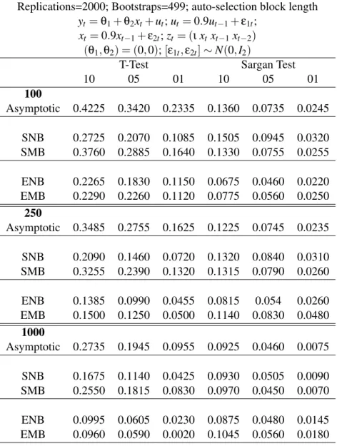
Results are reported in Table 1. The amount of dependence in the moment conditions is rela-tively high,ρ=0.9. The block length is set equal to the lag window in the HAC estimator, which is chosen using a data-dependent method (Newey and West (1994)). One immediate observation is that the asymptotic test-statistics severely over-reject the true null hypothesis. For example, with 100 observations the actual level for a 10%t-test is 42.25%. The actual level of theJ-test is closer to the nominal level, although there is still over-rejection. The block bootstrap, with block size averaging from 1.96 for 100 observations to 4.48 for 1,000 observations, reduces the amount of over-rejection of thet-test substantially. The greatest improvements for thet-test are with the stan-dard bootstrap. For theJ-test the empirical likelihood bootstrap produces actual size much closer to the nominal size than the alternatives. Interestingly, the overlapping bootstrap has worse size than the non-overlapping block bootstrap for thet-test.

(15)

5.1.2 Heteroscedastic Errors

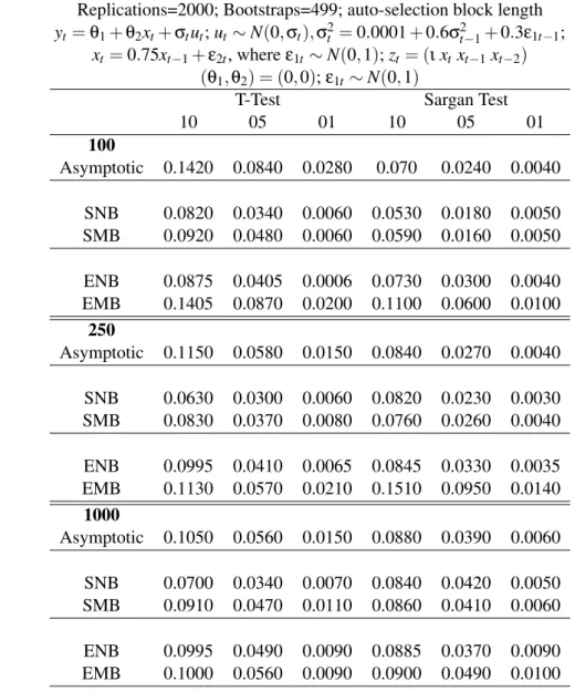
The subsequent DGP is the same as in the previous section with the addition of conditional heteroscedasticity, modeled as aGARCH(1,1). The DGP is:

yt=θ1+θ2xt+σtut for t=1, ...T, (15)

where(θ1,θ2) = (0,0), xt =0.75xt−1+ε1t, andut ∼N(0,σt). σt2=0.0001+0.6σ2t−1+0.3ε22t−1

andε∼N(0,I). The unconditional variance is 1. The instrument set iszt = [ιxtxt−1xt−2].

Results with 2,000 replications and 499 bootstrap samples are presented in Table 2. There are three sample sizes: 100, 250, and 1000. The actual size of the asymptotic tests are close to the nominal size for sample size 250 and greater. The moving block bootstrap tests have good size and the empirical likelihood bootstrap performs best out of the bootstrap procedures. Using the standard block bootstrap actually leads to more severe under-rejection of the true null hypothesis than the asymptotic tests.

5.2 Case II: Nonlinear Models

Two experiments are considered. First the chi-squared experiment from Imbens, Spady, and Johnson (1998). Second, the asset pricing DGP outlined in Hall and Horowitz (1996) and used by Gregory, Lamarche, and Smith (2002). Imbens, Spady, and Johnson (1998) also consider this DGP. In addition this section looks at the empirical likelihood bootstrap in a framework with dependent data. It is the case of nonlinear models where the asymptotict-test and J-test tend to severely over-reject.

5.2.1 Asymmetric Errors

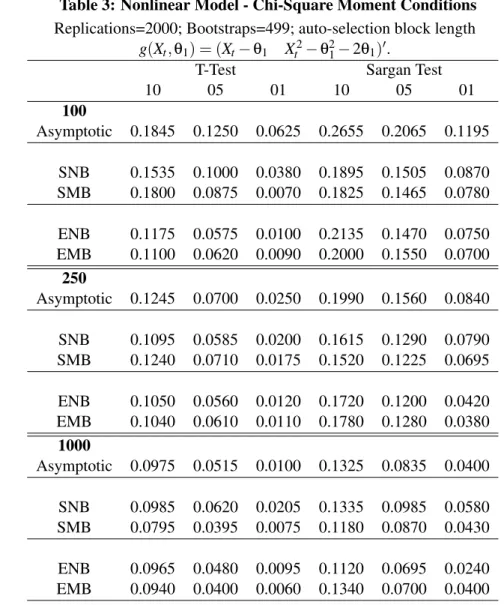
First consider a model with Chi-squared moments. Imbens, Spady, and Johnson (1998) provide evidence that average moment tests like theJ-test can substantially over-reject a true null hypothesis under a DGP with Chi-squared moments. The authors find that tests based on the exponential tilting parameter perform substantially better.

The moment vector is:

g(Xt,θ1) = (Xt−θ1 Xt2−θ21−2θ1)0.

(16)

Results for 2,000 replications and 499 bootstrap samples are presented in Table 3. There is se-vere over-rejection of the true null hypothesis when using the asymptotic distribution. The bootstrap procedures correct for this over-rejection; the empirical likelihood bootstrap performs very well for thet-tests. For small sample sizes the standard and empirical likelihood bootstrap both outperform the asymptotic approximation but there is still is an over-rejection.

5.2.2 Asset Pricing Example

Finally consider an asset pricing model with the following moment conditions.6_: E[exp(µ−θ(x+z) +3z)−1] =0, Ez[exp(µ−θ(x+z) +3z)−1] =0 . It is assumed that logxt =ρlogxt−1+ q (1−ρ2₎_ε_xt_, _z_t ₌_ρ_z_t−₁₊ q (1−ρ2₎_ε_zt

, whereεxtandεztare independent normal with mean 0 and variance 0.16. In the experimentρ=0.6.

Results for 2,000 replications and 499 bootstrap samples are presented in Table 4. Again, the asymptotic tests severely over-reject the true null hypothesis. The bootstrap procedures produce tests with reasonable size, especially for thet-tests. As was the case in the model with asymmetric errors, the empirical likelihood bootstrap performs best.

6 Conclusion

This paper extends the ideas put forth by Brown and Newey (2002) to bootstrap test-statistics based on empirical likelihood. Where Brown and Newey (2002) consider bootstrapping in aniid

context, this paper provides a proof of the first-order asymptotic validity of empirical likelihood block bootstrapping in the context of dependent data. Given the test-statistics considered, the size distortions of those tests based on the asymptotic distribution are severe, especially in the case of nonlinear moment conditions and substantial serial correlation. The empirical likelihood bootstrap largely corrects for these size distortions and produces promising results. This is especially true when the regression errors are non-spherical. The significance of using the empirical likelihood es-timator is that it satisfies the moment conditions identically while supplying a probability measure

(17)

under which these conditions hold. As highlighted by Brown and Newey (2002), the empirical like-lihood bootstrap is the same as the conventional bootstrap, except that it is based on a more efficient distribution estimator. Two possible avenues for future research include combining subsampling methods with empirical likelihood probability weights and establishing higher order improvements for the ENB and EMB.

7 Implementing the Block Bootstrap

The procedure for implementing the GMM overlapping (MBB) and empirical likelihood (EMB) bootstrap procedures are outlined below. The procedure is similar for the non-overlapping bootstrap.

1. Given the random sample(X1, ...,Xn), calculate ˆθusing 2-stage GMM

2. For EMB calculate ˆπo

i using equation (10)

3a. For EMB sample with replacement from{To

j(θˆ): j=1, . . . ,N}with probability{πˆoj : j=

1, . . . ,N}

3b. For MBB uniformly sample with replacement to get{X∗_}n

t=1= (X˜1, ...,X˜b)

4a. For EMB calculate the J-statistic (

J

∗

MBB,n) and t-statistic (Tnr∗)

4b. For MBB calculate J-statistic (

J

∗∗

MBB,n) and t-statistic (Tnr∗∗)

5. Repeat steps 3-4Btimes, whereBis the number of bootstraps. 6. Let ˆqπ_αbe a(1−α)percentile of the distribution ofT_nr∗ orT_nr∗∗

7. Letqπ

αbe a(1−α)percentile of the distribution of

J

MBB∗ ,nor

J

MBB∗∗ ,n

8. The bootstrap confidence interval forθ₀_ris ˆθ_nr±qˆπ

αn−1/2σˆnr

(18)

8 Mathematical Appendix

Assumptions A and B are a simplified version of Assumptions A and B in Gonc¸alves and White (2004), tailored to our GMM estimation framework.||x||pdenotes theLpnorm(E|Xnt|p)1/p. For a

(m×k)matrixx, let|x|denote the 1-norm ofx, so|x|=∑m_i=₁∑k_j=₁|xi j|.

Assumption A

A.1 Let (Ω,

F

,P) be a complete probability space. The observed data are a realization of a stochastic process{Xt:Ω→Rk,k∈N}, withXt(ω) =Wt(. . . ,Vt−1(ω),Vt(ω),Vt+1(ω), . . .),Vt:

Ω→Rv_,_v_∈_N_{, and}_W

t:∏∞τ=−∞Rv→Rl is such thatXt is measurable for allt.

A.2 The functionsg:Rk_×_Θ_→_Rm_{are such that}_g₍_·_,_θ₎_{is measurable for each}_θ_∈_Θ_{, a compact}

subset ofRp_,_p_∈_N_{, and}_g₍_X

t,·):Θ→Rmis continuous onΘa.s.-P,t=1,2, . . ..

A.3 (i)θ0is identifiably unique with respect toEg(Xt,θ)0W Eg(Xt,θ)and (ii)θ0is interior toΘ.

A.4 (i) {g(Xt,θ)} is Lipschitz continuous on Θ, i.e. |g(Xt,θ)−g(Xt,θo)| ≤Lt|θ−θo| a.s.-P, ∀θ,θo_∈_Θ_{, where sup}

tE(Lt) =O(1). (ii){∇g(Xt,θ)}is Lipschitz continuous onΘ.

A.5 For somer>2 : (i){g(Xt,θ)}isr-dominated onΘuniformly int, i.e. there existsDt:Rlt→R

such that|g(Xt,θ)| ≤Dt for allθinΘandDt is measurable such that||Dt||r≤∆<∞for all t. (ii){∇g(Xt,θ)}isr-dominated onΘuniformly int.

A.6 {V_t}is anα-mixing sequence of size−2r/(r−2), withr>2.

A.7 The elements of (i){g(Xt,θ)}are NED on{Vt}of size−1 uniformly on(Θ,ρ), whereρis

any convenient norm onRp_{, and (ii)}_{_∇_g₍_X

t,θ)}are NED on{Vt}of size−1 uniformly on

(Θ,ρ).

A.8 Σ≡limn→∞var(n−1/2∑nt=1g(Xt,θ0))is positive definite, andG≡limn→∞E(n−1∑nt=1∇g(Xt,θ0))

is of full rank.

Assumption B

B.1 {g(Xt,θ)}is 3r-dominated onΘuniformly int,r>2.

B.2 For some smallδ>0 and somer>2, the elements of{g(X_t,θ)}areL₂₊_δ−NED on{V_t}of size−(2(r−1))/(r−2)uniformly on(Θ,ρ);{Vt}is anα-mixing sequence of size−((2+

(19)

The following two lemmas are required to prove Theorems 1-3.

Lemma 1 Suppose Assumption A in the mathematical appendix hold. Thenθˆ−θ0→P0. If also

`→ ∞ and `=o(n), then θ∗∗

MBB−θˆ →P∗_,_P 0. If also Assumption B in Appendix hold and `=

o(n1/2−1/r), thenθ∗_MBB−θˆ →P∗_,_P0.

Lemma 2 Suppose Assumption A in the mathematical appendix hold,`→∞, and`=o(n). Then

θ∗∗

NBB−θˆ →P∗_,_P 0. If also `=o(n(r−2)/2(r−1)), then θ∗_NBB−θˆ →_P∗_,_P 0. Note that ` must satisfy

`=o(n1/2)because(r−2)/2(r−1)<1/2.

If we compare conditions on`, the condition with the NBB is slightly weaker because(r−2)/2(r−

1) =1/2−1/2(r−1)and 2(r−1)>r.

8.1 Proof of Lemma 1

The proof follows the proof of Theorem 2.1 of GW04, with two differences: (i) the tive function is a GMM objective function, and (ii) in the case of EMB, the bootstrapped objec-tive function depends on the probability weight ˆπo

i. ˆθ−θ0→P0 follows from applying Lemma

A.2 of GW04 to the GMM objective function, because conditions (a1)-(a3) in Lemma A.2 of GW04 are satisfied by Assumption A. The consistency of θ∗∗

MBB is proved by applying Lemma

A.2 of GW04. Their conditions (b1)-(b2) are satisfied by Assumptions A.2. Define ˜Qn(θ) =

(n−1∑n_t=₁g(X_t∗,θ))0W_n∗(n−1∑n_t=₁g(X_t∗,θ)), then their condition (b3) holds because sup_θ|Q∗∗_MBB_,_n(θ)−

˜

Qn(θ)| →P∗_,_P0 from a standard argument and sup_θ|Q˜_n(θ)−Q_n(θ)| →_P∗_,_P 0 by Lemmas A.4 and

A.5 of GW04.

We prove the consistency ofθ∗

MBBby approximating the EMB sample moment condition with an

uncentered MBB moment condition, namely, by showing sup_θ|b−1_∑b

i=1Tio∗(θ)−n−1∑nt=1g(Xt∗,θ)| →P∗_,_P

0 for suitably chosenTo∗

i (θ)’s andXt∗’s. Then the consistency of θ∗MBB follows from the proof of

the consistency ofθ∗∗

MBB. We will use the following result, which we prove later: Nπˆo_i =1+δni, max

1≤i≤N|δni|=oP(1). (16)

Partition the interval [0,1] into A1, . . . ,AN, where Ai = [πˆo0+· · ·+πˆoi−1,πˆ0o+· · ·+πˆoi] with

ˆ

πo

0=0. Partition the interval [0,1] into N sets, B1, . . . ,BN, where theBi’s are chosen such that µ(B_i) =1/Nand max₁_≤i≤Nµ(D_i) =o(N−1₎_{, where}_µ_{denotes the Lebesgue measure on}_[₀_,₁_]_{, and} Di= (Ai−Bi)∪(Bi−Ai), i.e., the symmetric difference betweenAi andBi. Such a construction

(20)

to drawiid uniform[0,1] random variablesU1, . . . ,Ub and setTko∗(θ) =Tio(θ) ifUk ∈Ai and set

˜

X∗

k =X˜i if Uk ∈Bi. Then we may write b−1∑bi=1Tio∗(θ) =b−1∑bk=1∑Ni=11{Uk ∈Ai}Tio(θ) and |b−1_∑b

i=1Tio∗(θ)−n−1∑nt=1g(Xt∗,θ)|=b−1∑bk=1∑Ni=11{Uk∈Di}|Tio(θ)|. Taking the bootstrap

ex-pectation of its supremum overθgivesE∗_sup

θb−1∑bk=1∑i=N11{Uk∈Di}|Tio(θ)| ≤E∗b−1∑k=b 1∑Ni=11{Uk∈ Di}supθ|Tio(θ)|=E∗∑Ni=11{U1 ∈Di}supθ|Tio(θ)| ≤ max1≤i≤Nµ(Di)∑Ni=1supθ|Tio(θ)|=oP(1).

Therefore, sup_θ|b−1∑b_i=₁T_io∗(θ)−n−1∑n_t=₁g(X_t∗,θ)|=oP∗_,_P(1), and the consistency ofθ∗_MBB

fol-lows.

It remains to show (16). First we showγo₍_θˆ_{) =}_O_P₍_`_n−1/2₎_{. In view of the argument in pp.}

100-101 of Owen (1990) (see also Kitamura (1997)),γo(θˆ) =OP(`n−1/2)holds if (a)`N−1∑Ni=1Tio(θˆ)Tio(θˆ)0→P

Σ, (b) `N−1_∑N

i=1Tio(θˆ) =OP(`n−1/2), and (c) max1≤i≤N|Tio(θˆ)|=oP(n1/2`−1). For (a), using a

mean value expansion and Assumption A.5 gives

¯ ¯ ¯ ¯ ¯`N−1 N

∑

i=1 T_io(θˆ)T_io(θˆ)0−`N−1 N

∑

i=1 T_io(θ0)Tio(θ0)0 ¯ ¯ ¯ ¯ ¯ ≤ |θˆ−θ0|2`N−1 N

∑

i=1 sup θ |∇T_io(θ)||T_io(θ)|=OP(n−1/2`) =oP(1). Define ¯G∗

n=n−1∑t=n 1g(Xt∗,θ0), then we have (cf. Lahiri (2003), p. 48)`N−1∑Ni=1Tio(θ0)Tio(θ0)0=

var∗(√nG¯∗_n) +`T¯nT¯n0, where ¯Tn=N−1∑Ni=1Tio(θ0). var∗( √

nG¯∗_n)−Σ→P0 from Corollary 2.1 of

Gonc¸alves and White (2002) (hereafter GW02). ¯Tnis equal to ¯Xγ,ndefined in p. 1371 of GW02 if we

replace theirX_twithg(X_t,θ₀). GW02 p.1381 shows ¯X_γ_,_n=o_P(`−1₎_{, and hence}_`_T_¯2

n =oP(1).

There-fore, `N−1_∑N

i=1Tio(θ0)Tio(θ0)0 →PΣ, and (a) follows. (b) follows from expanding Tio(θˆ)around

θ0 and using N−1∑Ni=1Tio(θ0) =n−1∑nt=1g(Xt,θ0) +Op(n−1`) (cf. Lemma A.1 of Fitzenberger

(1997)), and applying the central limit theorem. (c) holds because max₁_≤i≤N|To

i (θˆ)|=Oa.s.(N1/r)

from Lemma 3.2 of K¨unsch (1989) and`=o(n1/2−1/r₎_{. Therefore, we have}

γo(θˆ) =OP(`n−1/2), max 1≤i≤N|γ

o₍_θ_ˆ₎0_To

i (θˆ)|=oP(1). (17)

(16) follows from expandingNπo

i = (1+γo(θˆ)0Tio(θˆ))−1aroundγo(θˆ)0Tio(θˆ) =0.¤

8.2 Proof of Lemma 2

In view of the proof of Lemma 1, the consistency of θ∗∗_NBB holds because condition (b3) of Lemma A.2 of GW04 holds because sup_θ|Q˜n(θ)−Qn(θ)| →P∗_,_P0 by Lemmas 3 and 4.

(21)

In view of the proof of the consistency ofθ∗_MBBin Lemma 1,θ∗_NBBis consistent if

γ(θˆ) =OP(`n−1/2), max 1≤i≤b|γ(

ˆ

θ)0Ti(θˆ)|=oP(1). (18)

Equation (18) holds if (a) `b−1_∑b

i=1Ti(θˆ)Ti(θˆ)0 →P Σ, (b) `b−1∑bi=1Ti(θˆ) =OP(`n−1/2), and (c)

max1≤i≤b|Ti(θˆ)|=oP(n1/2`−1). (a) follows from expandingTi(θˆ) aroundθ0 and using Corollary

2. (b) follows from expandingTi(θˆ)aroundθ0and applying the central limit theorem. (c) follows

because max₁_≤i≤b|T_i(θˆ)|=O_a_._s_.(b1/r₎_and_`₌_o₍_n(r−2)/2(r−1)₎_._¤

8.3 Proof of Theorem 1

DefineH= (G0_{W G}₎−1_G0_W_Σ_{W G}₍_G0_{W G}₎−1_{, then the stated result follows from Polya’s theorem}

if we show√n(θˆ−θ0)→d N(0,H), √

n(θ∗

MBB−θˆ)→d∗ N(0,H) prob-P, and√n(θ∗∗_MBB−θˆ)→_d∗

N(0,H)prob-P. The limiting distribution of√n(θˆ−θ0)follows from a standard argument.

The proof of the asymptotic normality of θ∗

MBB and θ∗∗MBB uses Theorem 2.1 of Mason and

Newton (1992), who prove the consistency of generalized bootstrap (weighted bootstrap) proce-dures. We first derive the asymptotics of the EMB estimator. The first order condition for the EMB estimator is 0=b−1_∑b

i=1∇Tio∗(θ∗MBB)0WMBB∗ ,nb−1∑bi=1Tio∗(θ∗MBB). Expandingb−1∑bi=1Tio∗(θ∗MBB)

around ˆθand approximatingb−1_∑b

i=1∇Tio∗(θ)by n−1∑bi=1∇g(Xt∗,θ)as in the proof of Lemma 1

givesn1/2₍_θ∗

MBB−θˆ) =−(G˜0nWMBB∗ ,nG˜n)−1G˜0nWMBB∗ ,nn1/2b−1∑i=b 1Tio∗(θˆ), where ˜Gnis a generic

no-tation forG+oP∗_,_P(1). We proceed to rewriten1/2b−1∑b_i=₁T_io∗(θˆ)so that we can apply the results

in Mason and Newton (1992). Fori=1, . . . ,N, letwNibe the number of timesTio(θ)appears in a

bootstrap sample{To∗

k (θ)}bk=1. Conditional onX1, . . . ,Xn, anN-vectorwN= (wN1, . . . ,wNN)0

fol-lows a multinomial distribution such thatw_N∼Mult(b; ˆπo

1, . . . ,πˆoN). UsingwNiin conjunction with

∑N_i=₁πˆo

iTio(θˆ) =0 and b`=n, we may rewriten1/2b−1∑bi=1Tio∗(θˆ) =N−1/2∑Ni=1(N/b)1/2(wNi− bπˆo

i)`1/2Tio(θˆ).

Therefore, the asymptotic normality ofθ∗_MBBfollows if we show

N−1/2 N

∑

i=1

(N/b)1/2(wNi−bπˆoi)`1/2Tio(θˆ)→d∗ N(0,Σ) prob-P. (19)

We apply Theorem 2.1 of Mason and Newton (1992) to the left hand side of (19) with two minor changes. First, the weights in Theorem 2.1 of Mason and Newton (1992) do not depend on the data, whereas ourwNdepends on the data through ˆπoi. As Mason and Newton (1992) discuss on p.

1618, their Theorem 2.1 holds if the weights are exchangeable given the data. Second, in Mason and Newton (1992), condition (2.4) and result (2.7) hold P-almost surely. We can weaken both to

(22)

hold in P-probability becausexn→xin probability if and only if every subsequence of{xn}has a

further subsequence that converges almost surely tox (see, for example, Theorem 6.2 in p. 46 of Durrett (2005)).

For simplicity, we assumeTo

i (θ)to be a scalar without loss of generality. Note that our {N, `1/2_To

i (θˆ),(N/b)1/2(wNi−bπˆoi)} correspond to {kn,Xn,k,Yn,k} in Mason and Newton (1992).

From Theorem 2.1 of Mason and Newton (1992), (19) follows if we show (recall∑n_i=₁(wNi−bπˆoi) =

0 by construction) N−1 N

∑

i=1 (`1/2T_io(θˆ)−`1/2T¯o(θˆ))2→PΣ, N−1 N

∑

i=1 ((N/b)1/2(wNi−bπˆoi))2→P∗_,_P1, (20) where ¯To₍_θˆ_{) =}_N−1_∑N

i=1Tio(θˆ), and, for allτ>0,

(a) max 1≤i≤NU 2 Ni→P0, (b) max 1≤i≤NV 2 Ni→P∗_,_P0, (21) DN(τ) = N

∑

i=1 N

∑

j=1 U_Ni2V_{N j}2 1{NU_Ni2V_{N j}2 >τ} →P∗_,_P0, (22) where UNi= ` 1/2_To i (θˆ)−`1/2T¯o(θˆ) (∑N_i=₁(`1/2_To i (θˆ)−`1/2T¯o(θˆ))2)1/2 , VNi= (N/b) 1/2₍_w Ni−bπˆoi) (∑Ni=1((N/b)1/2(wNi−bπˆoi))2)1/2 . We proceed to check (20)-(22). The first part of (20) holds because (a) and (b) in the proof of Lemma 1 show `N−1_∑N

i=1Tio(θˆ)2 →P Σ and ¯To(θˆ) = OP(N−1/2). The second part of (20)

follows from applying Lemma 5 to the left hand side with r =2 because wN satisfies the

as-sumptions in Lemma 5. (a) of (21) follows from the first part of (20), ¯To₍_θˆ_{) =}_O_P₍_N−1/2₎_{, and}

max1≤i≤N|Tio(θˆ)|=oP(N1/2`−1), which is shown in (c) in the proof of Lemma 1. (b) of (21)

follows from Theorem 1 of Hoeffding (1951) in conjunction with the second part of (20) and Lemma 5 with r =4. Finally, (22) can be be shown by a similar argument to Corollary 2.2 of Mason and Newton (1992). For any ε ∈(0,1), from (b) of (21) we have, for sufficiently large N, with prob-P∗_{, prob-P greater than 1}₋_ε_, _D

N(τ) ≤∑Ni=1∑Nj=1UNi2VN j2 1{NUNi2 >τ/ε}=

∑N_i=₁U_Ni21{NU_Ni2 >τ/ε}. From the first part of (20) and the order of ¯To(θ), this is bounded by

Σ−1_N−1_∑N

i=1`Tio(θ0)21{NUNi2 >τ/ε}+oP(1). Consequently, choosingε sufficiently small gives D_n(τ)→_P∗_,_P 0 fromE`|T_io(θ₀)|2=O(1)(see Lemmas A.1 and A.2 of GW02) and the dominated

convergence theorem.

(23)

argument givesn1/2(θ∗∗_MBB−θˆ) =−(G˜0_nW_n∗∗G˜n)−1G˜0nWn∗∗n−1/2∑nt=1g∗(Xt∗,θˆ). Fori=1, . . . ,N, let w∗

Nibe the number of times ˜Xiappears in a bootstrap sample{X˜_k∗}b_k=₁. Conditional onX1, . . . ,Xn, an N-vectorw∗

N= (wN1, . . . ,wNN)0follows Mult(b; 1/N, . . . ,1/N). UsingN−1∑Ni=1Tio(θˆ) =n−1∑nt=1g(Xt,θˆ)+ OP(n−1`)(cf. Lemma A.1 of Fitzenberger (1997)), we may writen−1/2∑nt=1g∗(Xt∗,θˆ)

=N−1/2_∑N

i=1(N/b)1/2(w∗Ni−b/N)`1/2Tio(θˆ)+oP(1). Sincew∗Nsatisfies the assumptions in Lemma

5, repeating the proof for the EMB estimator with replacingwNbyw∗NgivesN−1/2∑i=N1(N/b)1/2(w∗Ni− b/N)`1/2_To

i (θˆ)→d∗N(0,Σ)prob-P, and the stated result follows.¤

The proof closely follows the proof of Theorem 1. Because we sample frombblocks, instead ofN, we use Corollary 1 in place of Lemma 5.

We first derive the asymptotics of the ENB estimator. Expanding the first order condition for the ENB estimator givesn1/2₍_θ∗

NBB−θˆ) =−(G˜0nWNBB∗ ,nG˜n)−1G˜0nWNBB∗ ,nn1/2b−1∑i=b 1Ti∗(θˆ), where ˜Gnis

a generic notation forG+oP∗_,_P(1). The required result follows if we shown1/2b−1∑b_i=₁T_i∗(θˆ)→_d∗

N(0,Σ)prob-P. Fori=1, . . . ,b, letwbi be the number of timesTi(θ)appears in a bootstrap sample {T∗

k(θ)}bk=1. Conditional onX1, . . . ,Xn, anb-vectorwb= (wb1, . . . ,wbb)0follows Mult(b; ˆπ1, . . . ,πˆb).

Using∑b_i=₁πˆiTi(θˆ) =0 andb`=n, we may rewriten1/2b−1∑bi=1Ti∗(θˆ) =b−1/2∑bi=1(wbi−bπˆi)`1/2Ti(θˆ).

From Theorem 2.1 of Mason and Newton (1992),b−1/2∑b_i=₁(wbi−bπˆi)`1/2Ti(θˆ)→d∗N(0,Σ)

prob-P follows if we show b−1 b

∑

i=1 (`1/2Ti(θˆ)−`1/2T¯(θˆ))2→PΣ, b−1 b

∑

i=1 (wbi−bπˆi)2→P∗_,_P1, (23) where ¯T(θˆ) =b−1_∑b

i=1Ti(θˆ), and, for allτ>0,

(a)max 1≤i≤bU 2 bi→P0, (b)max 1≤i≤bV 2 bi→P∗_,_P0, (24) D_b(τ) =

∑

b i=1 b

∑

j=1 U_bi2V_{b j}21{bU_bi2V_{b j}2 >τ} →P∗_,_P0, (25) whereUbi= (`1/2Ti(θˆ)−`1/2T¯(θˆ))(∑bi=1(`1/2Ti(θˆ)−`1/2T¯(θˆ))2)−1/2andVbi= (wbi−bπˆi)(∑Ni=1(wbi− bπˆi)2)−1/2.

We proceed to check (23)-(25). The first part of (23) holds because (a) and (b) in the proof of Lemma 2 show`b−1_∑b

i=1Ti(θˆ)2→PΣand ¯T(θˆ) =OP(n−1/2). The second part of (23) follows from

applying Corollary 1 withr=2. (a) of (24) follows from the first part of (23), ¯T(θˆ) =OP(n−1/2),

(24)

follows from Theorem 1 of Hoeffding (1951) in conjunction with the second part of (23) and Corol-lary 1 with r =4. Finally, (25) is shown by repeating the argument of the proof of (22) since

U2

bi=b−1`Ti(θ0)2(Σ−1+oP∗_,_P(1)), and we derive the asymptotics ofθ∗_NBB. The proof for the

stan-dard bootstrap estimatorθ∗∗

NBB is very similar and omitted.¤

The validity of the bootstrap Wald test is proven if we showS∗∗

n (θ∗),S∗MBB,n(θ∗),S∗NBB,n(θ∗)→P∗_,_P

Σfor any root-nconsistentθ∗. Using a similar argument to the consistency proof ofθ∗_MBB, we can showS∗

MBB,n(θ∗) is asymptotically equivalent in distribution toS∗∗n (θ∗) that is constructed from a

standard MBB sample. S∗∗

n (θ∗)→P∗_,_P Σ then follows from result (iii) in the proof of Theorem

3.1 of GW04. Similarly, S∗

NBB,n(θ∗)is asymptotically equivalent in distribution to S∗∗n (θ∗) that is

constructed from a standard NBB sample, which converges toΣfrom Corollary 2.

J

n→dχ2m−p ifWn→PΣ−1andn−1/2∑nt=1g(Xt,θ0)→d N(0,Σ), which follows from

Assump-tions A and B and a standard argument.

J

∗

MBB,n→d∗χ2_m−pprob-P becauseS∗_MBB_,_n(θ˜∗_MBB)→_P∗_,_PΣand

n1/2_b−1_∑b

i=1Tio∗(θˆ)→d∗N(0,Σ)prob-P.

J

_MBB∗∗ _,_n→_d∗χ2_m−pprob-P follows becauseS_n∗∗(θ∗∗_MBB)→_P∗_,_P

Σand we have shown in the proof of Theorem 1 thatn−1/2∑_t=n ₁g∗(Xt,θˆ)→d∗ N(0,Σ)prob-P. The

convergence of

J

∗

NBB,nand

J

NBB∗∗ ,nare proven by a similar argument. ¤

9 Auxiliary results

Lemma 3 (NBB uniform WLLN). Let{q∗

nt(·,ω,θ)}be an NBB resample of{qnt(ω,θ)}and assume: (a) For eachθ∈Θ⊂Rp_,_Θ_{a compact set, n}_∑n

t=1(q∗nt(·,ω,θ)−qnt(ω,θ))→0, prob-P∗n,ω, prob-P;

and (b)∀θ,θ0∈Θ,|qnt(·,θ)−qnt(·,θ0)| ≤Lnt|θ−θ0|a.s.-P, wheresupn{n−1∑t=n 1E(Lnt)}=O(1). Then, if`=o(n), for anyδ>0andξ>0,

lim n→∞P " P_n∗_,_ω Ã sup θ∈Θ n−1 ¯ ¯ ¯ ¯ ¯ n

∑

t=1 (q∗_nt(·,ω,θ)−q_nt(ω,θ)) ¯ ¯ ¯ ¯ ¯>δ ! >ξ # =0.

Proof The proof closely follows that of Lemma 8 of Hall and Horowitz (1996).¤

Lemma 4 (NBB pointwise WLLN). For some r>2, let {qnt :Ω×Θ→Rm:m∈N}be such that for all n,t, there exists D_nt:Ω→Rwith|q_nt(·,θ)| ≤D_nt for allθ∈Θand||D_nt||_r≤∆<∞. For eachθ∈Θ let{q∗

(25)

ξ>0and for eachθ∈Θ, lim n→∞P " P_n∗_,_ω Ã n−1 ¯ ¯ ¯ ¯ ¯ n

∑

t=1 (q∗_nt(·,ω,θ)−qnt(ω,θ)) ¯ ¯ ¯ ¯ ¯>δ ! >ξ # =0.

Proof Fixθ∈Θ, and we suppressθandω henceforth. Sinceq∗

nt is a NBB resample, E∗q∗nt = n−1_∑n

t=1qnt =q¯nand hence∑t=n 1(q∗nt−qnt) =∑nt=1(q∗nt−E∗qnt). From the arguments in the proof

of Lemma A.5 of GW04, the stated result follows if ||var∗₍_n−1/2_∑n

t=1q∗nt)||r/2=O(`) for some r>2. DefineUni=`−1∑`t=1qn,(i−1)`+t, the average of theith block. Since the blocks are

indepen-dently sampled, we have (cf. Lahiri (2003), p.48) var∗₍_n−1/2_∑n

t=1q∗nt) =b−1`∑i=b