ABSTRACT— this research was focused on a heterogeneous fleet of passenger ships multi-depot by using the genetic algorithm (GA) to solve a combinatorial problem i.e. vehicle routing problem (VRP). The objective of this study is to compare the roulette wheel selection, single cut point crossover, and shift neighborhood mutation with selection based on selection rate, single cut point crossover, and shift neighborhood mutation to minimize the sum of the fuel consumption travelled, the cost for violations of the ship draft and sea depth, and penalty cost for violations of the load factor; to maximize the number port of call; and to maximize load factor. Problem-solving in this study is how to generate feasible route combinations for rich VRP that meets all the requirements with the optimum solution. Route generated by roulette wheel selection, single cut point crossover, and shift neighborhood mutation could decrease fuel consumption about 17.8990% compared to selection rate, single cut point crossover, and shift neighborhood mutation about 18.8825%.
Index Terms—Vehicle Routing Problem; Genetic Algorithms; Multi-Depot; Roulette wheel selection, Rank & selection based on selection Rate
I. INTRODUCTION
Vehicle routing problem (VRP) is a classical combinatorial optimization problem. It is a key component of transportation management. It was first introduced to determine vehicle routes with minimum cost to serve a set of customers whose geographical coordinates and demands are known in advance [1]. A vehicle is required to visit each customer only once. Typically, vehicles are homogeneous and have the same capacity restriction.
VRP can be represented as the following graph-theoretic problem. Let G = (P, A) be a complete graph where P = {0, 1… n} is the vertex set and representing customers with the depot located at vertex 0; A is the arc set. Vertices j = {1, 2… n} correspond to the customers, each with a known non-negative demand, dj. A non-non-negative cost, cij, is associated
Ismail @ Ismail Yusuf Panessai is with Faculty of Art, Computing and Creative Industry, Tanjung Malim, Malaysia. (Corresponding author to provide phone: +60163756016; e-mail: [email protected]).
Muhammad Modi bin Lakulu, Asmara binti Alias, and Hafizul Fahri bin Hanafi are with Faculty of Art, Computing and Creative Industry, Tanjung Malim, Malaysia.
Siva Kumar A/L Subramaniam is with Dept. of Electronic & Computer Eng., Universiti Teknikal Malaysia Melaka, Melaka, Malaysia.
Husni Naparin is with STKOM Sapta Computer (SC), Balangan, Indonesia.
with each arc (i, j) ϵ A and represents the cost of traveling from vertex i to vertex j. If the cost values satisfy cij ≠ cjifor
all i, j ϵ P, then the problem is said to be an asymmetric VRP; otherwise, it is called asymmetric VRP. In some contexts, cijcan be interpreted as a travel time or travel cost.
The VRP consists of designing a set vehicle route with minimum cost, defined as the sum of the costs of the routes’ arcs such that:
• All vehicle routes start and end at the same depot • Each customer in P is visited exactly once by exactly
one vehicle
• Some side soft and hard constraints are satisfied MDVRP has been proposed to follow each depot stores and supplies various products and has a number of identical vehicles with the same capacity to serve customers who demand different quantities of various products [2]. Each vehicle starts the tour from its resided depot, delivers products to a number of customers, and returns to the same depot. One variant of the CVRP is the heterogeneous fleet vehicle routing problem (HVRP). In HVRP, the fleet is composed of a fixed number of vehicles with differences in their equipment, capacity, age or cost which the number of available vehicles is fixed as a priori [3]. The decision is how to be the best to utilize the existing fleet to serve customer demands.
Forward six formulations determined by Yaman [4] which are enhanced by valid inequalities and lifting; Choi & Tcha [5] presented a linear programming relaxation of which is solved by the column generation technique and used column generation technique which is enhanced by dynamic programming schemes; a branch-cut-and-price algorithm over an extended formulation that capable for solving HVRP proposed by Pessoa, et.al. [6] And a tabu search used approach using GENIUS for HVRP [7].
Developing an algorithm based on heuristics and followed by a local search procedure based on the steepest descent local search and tabu search [8] while three-phase heuristic developed by Dondo, et.al. [9] And an iterated local search based on heuristic proposed by Penna, et.al. [10]. A hybrid algorithm that composed by an iterated local search based on heuristic and a set partitioning formulation discussed by Subramanian, et.al. [11]. The set partitioning model was solved by means of a mixed integer programming solver that interactively calls the iterated local search heuristic during its execution.
An evolutionary hybrid meta-heuristic research combines
Increasing the Performance of Genetic
Algorithm by Using Different Selection:
Vehicle Routing Problem Cases
a parallel genetic algorithm with scatter search also presented by Ochi, et.al. [12], while a record-to-record travel metaheuristic published by Li, et.al. [13]. In addition, memetic algorithm to solve HVRP is proposed by Prins [14].
HVRP has been solved by implementing a threshold accepting procedure where a worse solution is only accepted if it is within a given threshold [15]; and provided an improved version in Tarantilis, et.al. [16]. A memory programming metaheuristic discussed by Li, et.al. [17] While tabu search algorithm to solve HFVRP used by Brandão [18].
Several simple heuristics have been developed by Nag, et.al. [19] And more advanced heuristic proposed by Chao, et.al. [20], tabu search by Cordeau & Laporte [21], while memetic algorithm to solve SDCVRP presented by Nagata & Bräysy [22].
AVRP is related to Asymmetric Travelling Salesman Problem (ATSP). It is a generalized traveling salesman problem in which distances between a pair of cities do not need to be equal in the opposite direction. The ATSP is an NP-hard problem, thus many meta-heuristic algorithms have been proposed to solve this problem, such as hybrid genetic algorithm by Choi, et.al. [23] And tabu search proposed by Basu, et.al. [24].
II.VEHICLE ROUTING PROBLEM MODEL
This study is on a heterogeneous fleet of passenger ships to solve multi-depot. The objective of the research problem consists of:
i. Minimum fuel consumption
The fuel consumption of each vehicle depends on the type is related with the type of engine used proposed by Ismail et. al. [25]:
* k* k* k*
k P T
f (1)
f k = Total fuel consumption served by ship k T k = Total voyage time by ship k
k r
L
= Total distance travelled for route r served by ship kvk = Speed of ship k
η = High Speed Diesel constant (0.16) Pk = Engine power of ship k (HP)
Φ = Number of engine Μ = Efficiency (0.8) Maximum number port of call
Number port of call of the route r that served by ship k donated by
rkii. Maximum load factor
Load factor of ship k in each path calculated by:
k k ij k
ij q
b (2)
k ij
b
= Load factor of ship k sailing from port i to port j in route rk ij
= Number of passenger in ship k sailing from port i to port j in route rqk = Capacity of ship k
Hard constraints are dealt with by removing the unfeasible route. Hard constraints in this study include: i. Fuel Port
A route must include at least one fuel port. ii. Travel Time
The maximum duration for each tour is called commission days,
T
which is 14 days for this case. Hence, ship must return to the depot withinT
. IfT
k is the ship’s voyage time, whileT
k
T
.iii.Travel Distance
Since each ship has a different fuel tank size. Hence, total distance travelled for route r served by ship k,
L
kr that it can travel is different. IfL
k is maximum allowed routing distance for ship k, whileL
kr
L
k.k
L
Calculated by:) 24 * ( * * *
* k
k k
k k
k v
P v
L
(3)
Where,
Lk = Maximum allowed routing distance for ship k θk = Maximum capacity tank of the ship k vk = Speed of ship k
η = High Speed Diesel constant (0.16) Pk = Engine power of ship k (HP)
Φk = Number of engine used in ship k μ = Efficiency (0.8)
A.Mathematical Model
Let, G = (P, A) be a graph, where P is the set of all ports, denoted by the nodes C (customer ports) and D (fuel ports) at which K is a set mix vehicles with capacity qk are based. A = {(i, j) │ i, j; i < j} is the set of arcs. Every arc (i, j) is associated with a non-negative distance matrix L=
l
ijk , which represents the asymmetric travel distance from port i to port j, i.e., lijmay be different from lji; i, j ∈ P.B. Notation
C = {1, 2… m} is a set of customer ports
D = {(m+1), (m+2)… (m+n)} is a set of fuel ports
P = CD = {1, 2… m, (m+1), (m+2)… (m+n)} is the set of all ports; n(P) = number of the ports
K = {1, 2… k} is a set of ship; n(K) = number of the ships. C. Parameter
hi = Sea depth of port i, i∈{1, 2, …,m+n } k
v
= Speed of ship i k
= Ship draft of ship i;i∈{1, 2… n (K)} ki
r
= Route i for ship k kij
f
= Fuel consumption for ship k to sail from port i to port jk r
f
= Fuel consumption for ship k to serve route r kij
k ij
T
= Travel time for ship k sailing from port i to port j and stay in port ik
T
= Total voyage time by ship kT
= Maximum allowed routing time (commission days)k ij
l
= Distance travelled for ship k sailing from port i to port j; lijmay be different from ljik ij
L
= Distance travelled for ship k sailing from port i to port j and back to port ik r
L
= Total distance travelled for route r served by ship kk
L
= Maximum allowed routing distance for ship k kij
b
= Load factor for ship k sailing from port i to port j kij
B
= Average load factor for ship k sailing from port i to port j and back to port ik r
B
= Average load factor for route r served by ship k kij
q = Available seat capacity of the ship k travel from ports i to j
k ij
= Number of passenger on board, travel from ports i to j
α = Penalty cost for violations of the ship draft and sea depth
β = Penalty cost for violations of the load factor ξ = Number port of call
D. Decision Variables
otherwise 0 route serving for used is ship if
1 k i
uk i otherwise 0 route in ship by served is port if 1 , r k i wk i r otherwise 0 where , depth sea with port from sailing draft ship with ship if
500 k δk i hi k hi
β is a variable for ship k sailing from port i to port j and back to port i by average load factor k
ij B otherwise 0 75 50 500 50 1000 k ij k ij B B
The problem is to construct route with minimum fuel consumption in feasible set of routes for each vehicle. The feasible route for ship k is to serve ports without exceeding the constraints:
1. Total travel time
T
kfor any vehicle is no longer than T 2. Total travel distanceL
ki for any vehicle is no longerthan
L
k3. The feasible route must include at least one fuel port The mathematical formulation is given in:
P i k ij P j K k P i k ij P j K k P i k ij k ij P j K k u u u f
minimize . . . (4)
(4) k
r
maximize
(5)k r
B
maximize
(6)1. All ports (customer and fuel port) i are serviced by ship k minimum at once
K k P i u P i k ij K k
, ,1 (7)
2. Travel time of the ship k is no longer than the maximum allowed routing time T , T = 14 days.
T Tk K k
(8)3. Total distance travelled for route i served by ship k is no longer than the maximum allowed routing distance of the ship k, then
L
ki
L
k.k k i K k L L
(9)4. Travel time of ship k equals to the distance travelled and divided by running speedvk.
k k k
v L
T (10)
5. The vehicle capacity constraint
P i k ij k ij i P j K k q uq . (11)
6. Ship k with ship draft δk sailing from port i with sea
depth hi and it is equal to α.
P i k hi P j K kx (12)
7. Ship k sailing from port i to port j and back to port i by average load factor
B
ijk and it is equal to β.
P i k ij P j K kB (13)
8. Route r served by ships k should possess a fuel-port
P j i k ij D p K k u p , 1. (14)
Three objectives in this study are minimum fuel consumption, maximum port of call and maximum load factor. All objective tested in different scenarios.
Minimum fuel consumption
In this case, the fitness value is the total fuel consumption of each ship. Obviously, it is a minimization problem, thus the smallest value is the best. The fitness function represents as Eq. (15):
1,000,000
*
1
1
k rf
f
(15) k rf
= Fuel consumption for ship k to serve route rMaximum number port of call
In this case, the fitness value is the total port of call of each route. Obviously, it is a maximization problem, thus the largest value is the best. The fitness function represents as Eq. (16):
k r
f
(16)k r
= Number port of call of the route r that served by ship kIn this case, the fitness value is the average of load factor of each route. Obviously, it is a maximization problem, thus the largest value is the best. The fitness function represents as Eq. (17):
k r
B
f
(17)k r
B
= Average load factor for route r served by ship k In this research, a classical selection method is used for solving routing problems, namely the roulette wheel selection. The selection process begins by spinning the roulette wheel n times; each time, a single chromosome is selected for a new population in the following 2 steps: Step 1: Generate a random number r in a range [0, 1]. Step 2: If r ≤ q1, then select the first chromosome s1otherwise, select the s-th chromosome (1 ≤ s ≤ n) such that qs-1 < r ≤ qs.
E. Selection
Selection is a process to select parent chromosomes and offspring based on the fitness value to form a new better generation to follow the objective function.
In this study, a classical selection method is used for solving routing problems, namely the roulette wheel selection. It is compared with proposed selection method; selection based on selection rate. The objective is to show the impact of the choice of a given operator on the efficiency of the methods.
1) Roulette Wheel Selection
Roulette wheel selection was selecting a new population with respect to the probability distribution based on their fitness values.
The roulette wheel selection can be constructed as follows: Calculate the fitness value fs of each chromosome s:
) (x f
fs (18)
Calculate the total fitness of population: s
f
F
pop_size
1 k
(19)
Calculate the selection probability ps of each chromosome: F
f
p s
s (20)
Calculate the cumulative probability qs of each chromosome s:
i s
s p
q
1 i
(21)
n = Number of population s = 1, 2, 3… n
2) Rank & Selection Based on Selection Rate
The selection proposed procedure is as follows: Step 1 : Generate a random number r in the range (0, 1]. Step 2 : If r < Ps then chromosome s is selected.
Step 3 : Check for the number of chromosomes not selected
Step 4 : Rank fitness of the current population. Choose the chromosome with the highest and the lowest fitness from the current population.
F. Mutation
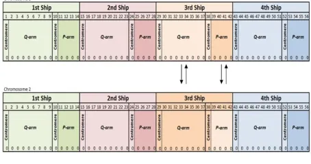
Shift neighbourhood is shift randomly genes code in a chromosome to a neighbour routes (i.e. neighbour is refer to the numbering of the routes). The steps for the shift neighbour mutation process in this study are as follows: Step 1: Select the genes in a route which will be generated
by mutation at random.
Step 2: Change the genes in a route with the next routes. Step 3: Genes in the first route exchanged with the second
[image:4.612.312.540.168.325.2]route, and genes in the second route exchanged with the third route.
Fig. 1. Shift neighbourhood mutation.
G. Crossover
[image:4.612.313.540.414.534.2]The type of crossover method used is single cut point crossover. Fig.2 is the description of the single cut point crossover.
Fig. 2. Single cut point crossover.
III. EXPERIMENT DESIGN
In order to show the effectiveness of GA, simulations were carried out. The algorithm proposes coded in Java and, using an Intel(R) Core(TM) i5 CPU M430 @ 2.27GHz. As methods compared have a stochastic behaviour, they have been tested 50 times on each benchmark for every GA operator.
mutation probability value set at 0.05; 0.2 and 0.3 (low), as well as with a population of 50 & 100.
The mutation probability values to vary by 0; 0.1; 0.2 so that 1 (from the lowest to the highest), and the number of populations varies from 8 to 100. Then, the combination of the mutation probability values and the number population set one by one, while the value for crossover probability is set to 0 byMungwattana [29] and also proposed by Volna [30]. Ghani, et.al. [31] Focused on very small mutation probability values (ie below 0.1), but with a large probability of crossover ranges from 0.9).
In this research, GA parameters used are population size: 100, maximum generation: 1000, crossover rate: 0.7, mutation rate: 0.5 and selection rate: 0.5. In addition, single cut point crossover, shift neighbourhood mutation, and two types of selection used, namely roulette wheel selection and rank & selection based on selection rate.
IV. RESULTS AND DISCUSSION
The aim of this research is to check the quality of solution obtained over algorithms in 11 benchmarks (as shown in Table 1) then check efficiency.
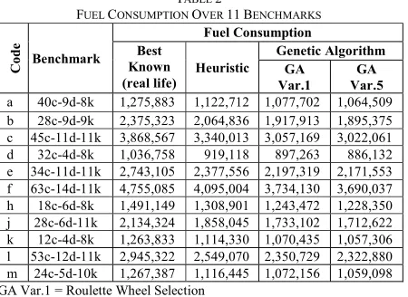
In this research, a computational study is carried out to study about performance of GA (GA Var.1 and GA Var.5) compared to the best know result and heuristic for solving the problem. All the result showed in the Table 2.
The quality of solution obtained by GA in 11 benchmarks was checked by Eq. (22).
100% X | |
solution Best know
ution known sol sed - Best Alg. propo Efficiency
Algorithm (22)
The percentage of efficiency for fuel consumption over 11 benchmarks showed in the Table 3.
Based on the Table 3; the average of efficiency algorithm over 11 benchmarks between roulette wheel selection, single cut point crossover, and shift neighbourhood mutation (GA Var.1) is about 17.8990%. While, selection based on selection rate, single cut point crossover, and shift neighbourhood mutation (GA Var.5) is about 18.8825%. It seemed that the best performance of GA algorithm by selection based on selection rate, single cut point crossover, and shift neighbourhood mutation (GA Var.5).
V.CONCLUSION
In this paper, the MDVRP, HFMVRP, SDCVRP and AVRP were studied and it is combined to solve ship routing. The best routing is minimum fuel consumption, maximum number of port of call and maximum load factor. In order to validate the algorithms, the mathematical programming model applied to 11 benchmarks. A computational study is carried out to compare of fuel consumption between roulette wheel selection, single cut point crossover, and shift neighbourhood mutation to rank & selection based on selection rate, multi-cut point crossover, and shift neighbourhood mutation. The result showed that the best performance algorithm is GA Var.5. Route generated by GA Var.5 could decrease fuel consumption about 18.8825% compared to GA Var.1 about 17.8990%.
This phenomenon proved that the GA proposed effectively used to solve the problem. Which the effective operator used are rank & selection based on selection rate, single cut point crossover, and shift neighbourhood mutation.
TABLE 3
THE PERCENTAGE OF EFFICIENCY FOR FUEL CONSUMPTION OVER 11 BENCHMARKS
C
od
e Benchmark
Fuel Consumption Best
Known (real
life)
Heuristic
Genetic Algorithm GA
Var.1 GA Var.5
a 40c-9d-8k 0 12.0051 15.5328 16.5669 b 28c-9d-9k 0 13.0714 19.2567 20.2056 c 45c-11d-11k 0 13.6628 20.9741 21.8816 d 32c-4d-8k 0 11.3469 13.4549 14.5286 e 34c-11d-11k 0 13.3261 19.8966 20.8630 f 63c-14d-11k 0 13.8816 21.4708 22.3981 h 18c-6d-8k 0 12.2220 16.6098 17.6239 j 28c-6d-11k 0 12.9446 18.7985 19.7581 k 12c-4d-8k 0 11.8293 15.3025 16.3413 l 53c-12d-11k 0 13.4536 20.1877 21.1332 m 24c-5d-10k 0 11.9097 15.4042 16.4346 Average 12.6957 17.8990 18.8825 GA Var.1 = Roulette Wheel Selection
GA Var.5 = Rank & Selection Based on Selection Rate TABLE 1
BENHMARKS FOR GAOPERATOR Benchmark
Number of
Fuel Consumption
Port Vehicle
Customer Fuel
40c-9d-8k 40 9 8 1,275,883
28c-9d-9k 28 9 9 2,375,323
45c-11d-11k 45 11 11 3,868,567
32c-4d-8k 32 4 8 1,036,758
34c-11d-11k 34 11 11 2,743,105
63c-14d-11k 63 14 11 4,755,085
18c-6d-8k 18 6 8 1,491,149
28c-6d-11k 28 6 11 2,134,324
12c-4d-8k 12 4 8 1,263,833
53c-12d-11k 53 12 11 2,945,322
24c-5d-10k 24 5 10 1,267,387
TABLE 2
FUEL CONSUMPTION OVER 11BENCHMARKS
C
od
e
Benchmark
Fuel Consumption Best
Known
(real life) Heuristic
Genetic Algorithm GA
Var.1
GA Var.5 a 40c-9d-8k 1,275,883 1,122,712 1,077,702 1,064,509 b 28c-9d-9k 2,375,323 2,064,836 1,917,913 1,895,375 c 45c-11d-11k 3,868,567 3,340,013 3,057,169 3,022,061 d 32c-4d-8k 1,036,758 919,118 897,263 886,132 e 34c-11d-11k 2,743,105 2,377,556 2,197,319 2,171,553 f 63c-14d-11k 4,755,085 4,095,004 3,734,130 3,690,037 h 18c-6d-8k 1,491,149 1,308,901 1,243,472 1,228,350 j 28c-6d-11k 2,134,324 1,858,045 1,733,102 1,712,622 k 12c-4d-8k 1,263,833 1,114,330 1,070,435 1,057,306 l 53c-12d-11k 2,945,322 2,549,070 2,350,729 2,322,880 m 24c-5d-10k 1,267,387 1,116,445 1,072,156 1,059,098 GA Var.1 = Roulette Wheel Selection
[image:5.612.71.296.539.703.2]REFERENCES
[1] G. B. Dantzig and J. H. Ramser, “The Truck Dispatching Problem,”
Management Science, vol. 6, pp.80-91, 1959.
[2] H. C. W. Lau, T. M. Chan, W. T. Tsui, and W. K. Pang, “Application of Genetic Algorithms to Solve the Multi Depot Vehicle Routing Problem,” Transactions on Automation Science and Engineering, vol. 7, pp. 383-392. 2010.
[3] E. D. Taillard, “A Heuristic Column Generation Method for the Heterogeneous Fleet VRP,” RAIRO, vol.33, pp. 1–14, 1999. [4] H. Yaman, “Formulations and Valid Inequalities for the
Heterogeneous Vehicle Routing Problem,” Mathematical Programming, vol. 106, pp. 365–390, 2006.
[5] E. Choi and D. W. Tcha, “A Column Generation Approach to the Heterogeneous Fleet Vehicle Routing Problem,” Computers and Operations Research, vol. 34, pp.2080–2095, 2007.
[6] A. Pessoa, E. Uchoa and M. Poggi de Aragão, “A Robust Branch-Cut-and-Price Algorithm for the Heterogeneous Fleet Vehicle Routing Problem,” Network, vol.54, pp.167–177. 2009.
[7] M. Gendreau, G. Laporte, C. Musaraganyi and E. D. Taillard, “A Tabu Search Heuristic for the Heterogeneous Fleet Vehicle Routing Problem,” Computers and Operations Research, vol.26, pp.1153– 1173, 1999.
[8] C. Prins, “Efficient Heuristics for the Heterogeneous Fleet Multi Trip VRP with Application to a Large-Scale Real Case,” Journal of Mathematical Modelling and Algorithms, vol.1, pp. 135–150, 2002. [9] R. Dondo and J. Cerdá, “A Cluster-Based Optimization Approach for
the Multi-Depot Heterogeneous Fleet Vehicle Routing Problem With Time Window,” European Journal of Operational Research, vol.176, pp.1478-1507, 2007.
[10] P. H. V. Penna, A. Subramanian, and L. S. Ochi, “An Iterated Local Search Heuristic for the Heterogeneous Fleet Vehicle Routing Problem, “ Journal of Heuristics, 2013.
[11] A. Subramanian, P. H. V. Penna, E. Uchoa and L. S. Ochi, “A hybrid algorithm for the Heterogeneous Fleet Vehicle Routing Problem,”
European Journal of Operational Research, vol.221, pp.285–295, 2012
[12] L. S. Ochi, D. S. Viana, L. Drummond, and A. O. Victor, “A Parallel Evolutionary Algorithm for the Vehicle Routing Problem with Heterogeneous Fleet,” Future Generation Computation System, vol.14, pp.285–292, 1998.
[13] F. Li, B. L. Golden, and E. Wasil, “A Record-to-Record Travel Algorithm for Solving the Heterogeneous Fleet Vehicle Routing Problems,” Computers and Operations Research, vol.34, pp.2734– 2742, 2007
[14] C. Prins, “Two Memetic Algorithms for Heterogeneous Fleet Vehicle Routing Problems, “ Eng.Appl.Artif.Intell. vol.22, pp.916–928, 2009 [15] C. D. Tarantilis, C. T. Kiranoudis, and V. S. Vassiliadis, “A List-Based Threshold Accepting Metaheuristic for the Heterogeneous Fixed Fleet Vehicle Routing Problem,” Journal of the Operational Research Society, vol.54, pp.65–71, 2003.
[16] C. D. Tarantilis, C. T. Kiranoudis and V. S. Vassiliadis, “A Threshold Accepting Metaheuristic for The Heterogeneous Fixed Fleet Vehicle Routing Problem,” Journal of the Operational Research Society, vol.152, pp.148–158, 2004
[17] X. Li, P. Tian, and Y. P. Aneja, “An Adaptive Memory Programming Metaheuristic For the Heterogeneous Fixed Fleet Vehicle Routing Problem,” Transport. Res.Pt.E, vol.46, pp.1111–1127, 2010. [18] J. Brandão, “A Tabu Search Algorithm for The Heterogeneous Fixed
Fleet Vehicle Routing Problem, ”Computers and Operations Research, vol.38, pp.140–151, 2011
[19] B. Nag, B. L. Golden, and A. Assad, “Vehicle Routing with Site Dependencies,” Vehicle routing: methods and studies, pp.149–159, 1988.
[20] I. M. Chao, B. Golden , and E. Wasil, “A Computational Study of a New Heuristic for the Site-Dependent Vehicle Routing Problem,”
INFOR, vol.37, pp.319-355, 1999.
[21] J. F. Cordeau and G. Laporte, ”A Tabu Search Algorithm for the Site Dependent Vehicle Routing Problem with Time Windows,” INFOR, vol. 39, pp.292-300, 2001
[22] Y. Nagata and O. Bräysy, “Edge Assembly-Based Memetic Algorithm for the Capacitated Vehicle Routing Problem,” Networks, vol.54, pp. 205–215, 2009
[23] I. C. Choi, S. I. Kim and H. S. Kim, “A Genetic Algorithm with a Mixed Region Search for the Asymmetric Travelling Salesman
Problem,” Computers and Operations Research, vol.30, pp. 773– 786, 2003
[24] S. Basu, R. S. Gajulapalli, and D. Ghosh, “Implementing Tabu Search to Exploit Sparsity in ATSP Instances,” Indian Institute of Management, W.P,2008.
[25] I. Yusuf, M. S. Baba and N. Iksan, “Applied Genetic Algorithm for Solving Rich VRP”, Applied Artificial Intelligence, Vol. 28, No.10, pp.957-991, 2014.
[26] S. N. Kumar and R. Panneerselvam, ”Development of an efficient Genetic Algorithm for the time dependent VRP with time windows”.
American Journal of Operations Research, vol.7. pp.1-25, 2016. [27] H. Bae and I. Moon, ”Multi-depot VRP with time windows
considering delivery and installation vehicles”. Applied Mathematical Modelling, vol.40. pp. 6536–6549, 2016
[28] H. Kocha, T. Henke, and G. Wäscher, ”A Genetic Algorithm for the multi-compartment VRP with flexible compartment sizes.” Working paper no. 4. Faculty of economics and management, universität magdeburg, 2016.
[29] A. Mungwattana, K. Soonpracha and T. Manisri, ” A Practical Case Study of a Heterogeneous Fleet VRP with Various Constraints”.
Proceedings of the 2016 International Conference on Industrial Engineering and Operations Management, pp.948-957, 2016. [30] E. Volna, ”Genetic Algorithm for the VRP,” Proceeding of
International Conference of Numerical Analysis and Applied Mathematics ICNAAM , vol. 4. pp.120002.1 – 120002.2016. [31] N. E. A. Ghani, S. R. Shariff and S. M. Zahari, ”An alternative
algorithm for VRP with time windows for daily deliveries,” Advances in Pure Mathematics,pp.342-350, 2016.
Ismail @ Ismail Yusuf Panessai received the diploma from the Polytechnic UNHAS Indonesia, bachelor in manufacturing (robotic, automation) UJ Indonesia, master science from Department of Artificial Intelligence in the Technical University UTeM Malaysia, and PhD from Department of Artificial Intelligence in University of Malaya. His main research interests include Artificial Intelligence in education; and Artificial Intelligence (Evolutionary Algorithm, Meta-heuristic, Expert System, and Fuzzy Logic System) and their application in decision making, operation research, vehicle routing problem (logistics/transportation) and control systems.