An alternating segment Crank–Nicolson parallel difference scheme for the time fractional sub diffusion equation

R E S E A R C H

Open Access

An alternating segment Crank–Nicolson

parallel difference scheme for the time

fractional sub-diffusion equation

Lifei Wu

_{, Xiaozhong Yang}

_{and Yanhua Cao}

*_{Correspondence:}

[email protected]

1_{School of Mathematics and}

Physics, North China Electric Power University, Beijing, China

Abstract

In this paper, an alternating segment Crank–Nicolson (ASC-N) parallel difference scheme is proposed for the time fractional sub-diffusion equation, which consists of the classical Crank–Nicolson scheme, four kinds of Saul’yev asymmetric schemes, and alternating segment technique. Theoretical analysis reveals that the ASC-N scheme is unconditionally stable and convergent by mathematical induction method. Finally, the theoretical analysis is verified by numerical experiments, which show that the ASC-N scheme is efficient for solving the time fractional sub-diffusion equation.

Keywords: Time fractional sub-diffusion equation; Alternating segment Crank–Nicolson scheme; Stability; Convergence; Parallel computing

1 Introduction

At present, the research on the fractional order differential and integral equations is at-tracting more and more attention. This kind of fractional order differential and integral equations are widely used in various fields of science and engineering [1,2]. Fractional derivatives have become an important tool to describe various complex mechanical be-haviors [3–5]. Most of fractional differential and integral equations cannot be solved an-alytically [6,7]. It is necessary and important to develop numerical methods for solving fractional differential and integral equations [8–10].

In recent years, many scholars have studied the numerical algorithms of fractional dif-fusion equation. The finite difference method is still dominant among the existing algo-rithms now. A class of unconditionally stable and convergent implicit difference approxi-mate methods for time fractional diffusion equation was constructed by Zhuang Pinghui et al. [11]. Charles Tadjeran et al. [12] examined a second order accurate numerical method in time and in space to solve a class of initial-boundary value fractional diffusion equa-tions with variable coefficients. The classical Crank–Nicholson (C-N) method and spatial extrapolation are used to obtain temporally and spatially second order accurate numeri-cal estimates [12]. Chen Changming et al. [13] presented implicit and explicit difference methods for solving the two-dimensional anomalous subdiffusion equation, and applied a new multivariate extrapolation to improve the accuracy [13]. Zhang, Pu et al. [14] con-structed a Crank–Nicolson-type difference scheme for fractional subdiffusion equation

with spatially variable coefficient [14]. Baleanu et al. [15] discussed the motion of a bead on a wire by fractional calculus [15]. They solved the fractional Euler–Lagrange equation numerically by using a discretization technique based on a Grünwald–Letnikov approx-imation for the fractional derivative. Jajarmi et al. [16] investigated an efficient iterative scheme with low computational effort for the optimal control of nonlinear fractional or-der dynamic systems with external persistent disturbances [16]. Hajipour et al. [17] pro-vided a new nonstandard finite difference scheme to study the dynamic treatments of a class of fractional chaotic systems and stability analysis of fractional order systems [17]. By combining the implicit difference scheme and the preconditioned conjugate gradient method, Wang Hong et al. [18,19] gave a fast implicit difference method for the two/three-dimensional fractional diffusion equation. The method has a computational work count of

O(NlogN) per iteration and a memory requirement ofO(N) [18,19]. Gao Guanghua et al. [20] derived a compact finite difference scheme for the sub-diffusion equation, which is fourth order accuracy compact approximate for the second order space derivative [20]. Gao Guanghua et al. [21] developed two higher order difference schemes for numeri-cally solving the one-dimensional time distributed-order fractional wave equations, one of which is the second order convergence in time and fourth order convergence in both space and distributed order [21]. Yaseen et al. [22] proposed a finite difference scheme with cubic trigonometric B-spline functions for time fractional diffusion-wave equation with reaction term [22]. The scheme is unconditional stable and convergent. Zaky et al. [23] proposed an efficient numerical algorithm for solving the variable order fractional Galilei advection-diffusion equation [23]. The method has the advantage of transforming the problem into the solution of a system of algebraic equations, which greatly simplifies it.

However, the existing serial implicit difference schemes are of relatively high computa-tional complexity and relatively low computacomputa-tional efficiency. With the rapid development of multi core and cluster technology, parallel computing is one of the main techniques to improve the efficiency of numerical calculation [24–27]. Zhang Baolin et al. proposed the idea which uses the Saul’yev asymmetric scheme to construct a segment implicit scheme, and the alternative technique to establish a variety of explicit-implicit or implicit alternat-ing parallel methods. The methods have been well applied to numerically solve integer partial differential equations [28–31].

Some progress in parallel algorithms of fractional order partial differential equations has been made. Most of the algorithms are studied on the parallel algorithm of alge-braic equations from the perspective of numerical algebra. Kai Diethelm [32] proposed to implement the fractional version of the second order Adams–Bashforth–Moulton method on a parallel computer and discussed the precise nature of parallel method [32]. Gong Chunye et al. [33,34] proposed an efficient parallel for Riesz and Caputo fractional reaction-diffusion equation respectively. The parallel solver involves the parallel tridiago-nal matrix vector multiplication, vector vector addition [33–35]. Sweilam et al. [36] con-structed a class of parallel C-N difference schemes for time fractional parabolic equations. The core of the method is to use the precondition conjugate gradient method to solve

In this paper, we construct an alternating segment C-N (ASC-N) difference scheme for time fractional sub-diffusion equation. The four kinds of Saul’yev asymmetric schemes and the classical C-N scheme are proposed. Then we use the four kinds of Saul’yev asym-metric scheme and the classical C-N scheme to construct an ASC-N scheme by the alter-nating segment technology. Using the mathematical induction method, we prove that the ASC-N scheme is unconditionally stable and convergent. Finally, the theoretical analysis is verified by numerical experiments, which show that the ASC-N scheme is effective for solving time fractional sub-diffusion equation.

2 Time fractional sub-diffusion equation

In this paper, we consider the time fractional sub-diffusion equation of the form [2,3]

∂α_u(x,t) ∂tα =

∂2_u(x,t)

∂x2 , 0≤x≤L, 0≤t≤T. (1)

Initial boundary conditions

u(0,t) =u(L,t) = 0, 0≤t≤T,

u(x, 0) =f(x), 0≤x≤L,

where∂α_∂u_t(αx,t)(0 <α< 1) denotes the Caputo fractional derivative of orderαof the function

u(x,t): ∂α_u(x,t)

∂tα = 1 (1 –α)

t

0

∂u(x,ξ) ∂ξ

dξ

(t–ξ)α. (2)

By taking the finite sine transform and Laplace transform, the analytical solution for equation (1) with the boundary conditions as above is obtained as [3]

u(x,t) = 2

L

∞

n=1

Eα

–a2n2tαsin(anx) t

0

f(r)sin(anr)dr, (3)

whereEα(z) is a Mittag-Leffler function,Eα(z) =

∞

k=0 z

k (αk+1),a=

π

L.

Some special Mittag-Leffler type functions are listed as follows:

E1(–z) =e–z, E2

–z2=cos(z),

E1 2(z) =

∞

k=1

zk

(k₂+ 1)=e

z2_erfc(–z), (4)

whereerfc(z) is the error function complement defined byerfc(z) =√2

π ∞

z e–t

2

dt.

3 The ASC-N scheme of fractional sub-diffusion equation

In this section, we first definetk=kτ,k= 0, 1, 2, . . . ,N, andxi=ih,i= 0, 1, 2, . . . ,M, where

τ =T_N,h=_ML are time and space steps, respectively. Letuk

i be the numerical approximation

The time fractional derivative term can be approximated by the following scheme:

Four kinds of Saul’yev asymmetric scheme are constructed for equation (1).

Lα_h,τu(xi,tk+1) =

Figure 1Point diagram of the ASC-N scheme

The C-N scheme also can be rewritten as follows. Whenk= 0,

–1 2u

1

i+1+ (1 +r)u1i –

1 2ru

1

i–1

=1 2ru

0

i+1+ (1 –r)u0i +

1 2ru

0

i–1.

Whenk> 0,

–1 2u

k+1

i+1 + (1 +r)uki+1–

1 2ru

k+1

i–1

=1 2ru

k

i+1–ruki +

1 2ru

k i–1+

k–1

j=0

cjuki–j+bku0i.

The design of the ASC-N scheme for equation (1) is as follows. Suppose the numerical value ofmgrid points needs to be calculated on each time layer. Letm=Al(A,lare inte-gers,Ais odd, andA≥3,l≥3).mgrid points will be divided intoAsegments, which is namedS1,S2, . . . ,SAin turn. In order to facilitate the description, setm= 25,l= 5. The

de-sign of ASC-N scheme’s segmentation is described by Fig.1. We use×to denote the C-N scheme in Fig.1.S1,S5have one inner boundary point (i= 5,i= 21), and four inner points

(i= 1, 2, 3, 4,i= 22, 23, 24, 25), respectively. S2, S3, S4 have two inner boundary points

(i= 6, 10,i= 11, 15,i= 16, 20) and three inner points (i= 7, 8, 9,i= 12, 13, 14,i= 17, 18, 19), respectively. We apply the C-N scheme at inner points, apply alternately the Saul’yev asym-metric scheme at inner boundary points in order to contact other inner points. Specifi-cally, at inner boundary points (5,k+ 1), (15,k+ 1), (10,k+ 2), (20,k+ 2) and (6,k+ 1), (16,k+ 1), (11,k+ 2), (21,k+ 2), we respectively apply Saul’yev asymmetric schemes (6), (7). At inner boundary points (10,k+ 1), (20,k+ 1), (5,k+ 2), (15,k+ 2) and (11,k+ 1), (21,k+ 1), (6,k+ 2), (16,k+ 2), we respectively apply Saul’yev asymmetric schemes (8), (9). And we alternately apply (6) and (8), (7) and (9) at different time steps. Therefore, atk+ 1 time step the space region will be divided into three segments (S1,S2andS3,S4andS5),

G(1)_2l =

diagonally dominant matrices. Therefore, we can get that ASC-N scheme (12) for time fractional sub-diffusion equation is uniquely solvable.

4 Theoretical analysis of the ASC-N scheme

4.1 Stability analysis of the ASC-N scheme

In order to discuss the stability of the ASC-N scheme, we need the following Kellogg lemma [24].

Lemma 1 If ρ > 0 and P is a nonnegative real matrix, then (ρI+P)–1 _{exists and} (ρI–P)(ρI+P)–12≤1.

Lemma 2 The matrices G1and G2of the ASC-N scheme are nonnegative real matrixes.

IfG1andG2meet thatG1+G1T,G2+G2Tare nonnegative real matrices, then Lemma2

real matrices. Sufficient and necessary conditions for the establishment of Lemma2are

G(1)_l +G(1)_l T,G(2)_l +G(2)_l T,G2l+G2lT,G(1)2l +G

(1) 2l

T

,G(2)_2l +G(2)_2lTare nonnegative real matrixes.

G2l+GT2l=

⎛ ⎜ ⎜ ⎜ ⎜ ⎜ ⎜ ⎜ ⎜ ⎜ ⎜ ⎜ ⎜ ⎜ ⎜ ⎜ ⎜ ⎜ ⎜ ⎜ ⎜ ⎝

2 –2

–2 4 –2

. .. ... ... –2 4 –2

–2 6 –4

–4 6 –2 (l+ 1)th line

–2 4 –2

. .. . .. . ..

–2 4 –2

–2 2 ⎞ ⎟ ⎟ ⎟ ⎟ ⎟ ⎟ ⎟ ⎟ ⎟ ⎟ ⎟ ⎟ ⎟ ⎟ ⎟ ⎟ ⎟ ⎟ ⎟ ⎟ ⎠

2l×2l

,

G2l+G2lTis diagonally dominant three diagonal matrix, and the main diagonal elements

are positive real numbers. SoG2l+G2lT is a nonnegative real matrix. In the same way,

we can prove thatG(1)_l +G(1)_l T,G(2)_l +G(2)_l T,G(1)_2l +G(1)_2lT,G₂(2)_l +G₂(2)_lTare nonnegative real matrices. Therefore,G1+G1T,G2+G2T are nonnegative real matrices. In other words,

G1andG2are two nonnegative real matrices.

From the definitions ofG(1)_l ,G(2)_l ,G₂(1)_l, andG₂(2)_l, we can know thatG(1)_l andG(2)_l have the same eigenvalues,G(1)_2l andG₂(2)_l have the same eigenvalues. Therefore,G1andG2have the

same eigenvalues, andrG12=rG22≥0.

The growth matrix of the ASC-N scheme for time fractional sub-diffusion equation is

T= (I+rG2)–1(I–rG1)(I+rG1)–1(I–rG2).

We can easily obtain estimates of the growth matrix by Lemmas1and2. Let

ˆ

T = (I+rG2)T(I+rG2)–1

= (I–rG1)(I+rG1)–1(I–rG2)(I+rG2)–1,

then

T2= ˆT2=(I–rG1)(I+rG1)–1(I–rG2)(I+rG2)–1₂≤1.

We suppose thatu˜k_i (i= 0, 1, 2, . . . ,M;k= 0, 1, 2, . . . ,N) is the approximate solution of ASC-N scheme (12), the errorε˜_ik=u˜k

i –uki,Ek= [εk1,εk2, . . . ,εkM–1]satisfies

(I+rG2)E1= (I–rG1)E0,

⎧ ⎨ ⎩

(I+rG1)Ek+1= (c0I–rG2)Ek+c1Ek–1+· · ·+ck–1E1+bkE0,

(I+rG2)Ek+2= (c0I–rG1)Ek+1+c1Ek+· · ·+ckE1+bk+1E0,

Fork= 1,λ1,λ2are the eigenvalues ofrG1,rG2, respectively.

T2=(I–rG1)(I+rG1)–1(I–rG2)(I+rG2)–1₂=max

1 –λ1

1 +λ2

2

≤1, (I+rG2)–1(I–rG1)₂=max

1 –λ2

1 +λ1

≤1, E1₂=(I+rG2)–1(I–rG1)E0₂

≤(I+rG2)–1(I–rG1)₂·E0₂≤E0₂.

Fork= 2,

E2₂ =(I+rG1)–1

(c0I–rG2)E1+b1E0 ₂ ≤(I+rG1)–1₂·(c0I–rG2)E1₂+b1

·E0₂

≤max|c0–λ1|+b1

1 +λ2

_E0

2.

Whenc0≥b1,

|c0–λ1|+b1

1 +λ2

=c0–λ1+b1 1 +λ2

=1 –λ1 1 +λ2

≤1.

Whenc0≤b1, 0 <b< 1⇒–1 < 2b1– 1 < 1,

|c0–λ1|+b1

1 +λ2

=λ1–c0+b1 1 +λ2

=λ1+ 2b1– 1 1 +λ2

≤1.

Therefore, we have

E2₂≤max|c0–λ1|+b1

1 +λ2

·E0₂≤E0₂.

Fork= 3,

E3₂ =(I+rG2)–1

(c0I–rG1)E2+c1E1+b2E0 ₂

=(I+rG2)–1₂·(c0I–rG1)E2+c1E1+b2E0₂ ≤(I+rG1)–1₂·(c0I–rG2)₂+c1+b2

·E0₂

≤(I+rG1)–1₂·(c0I–rG2)₂+b1

·E0₂

≤max|c0–λ1|+b1

1 +λ2

_E0

2

≤E0₂.

Suppose thatEj

2≤ E02,j≤2k. We have

E2k+1₂=(I+rG1)–1

(c0I–rG2)E2k+c1E2k–1+· · ·+b2kE0 ₂

≤(I+rG1)–1₂·

c0I–rG22+c1+· · ·+b2k

=(I+rG1)–1₂·

Theorem 1 ASC-N scheme(12)for time fractional sub-diffusion equation(1)is uncondi-tionally stable.

4.2 Accuracy of the ASC-N scheme

The ASC-N scheme will be expanded as the Taylor series at the point (xi,tk+1). Letu(xi,tk)

be the exact solution of the time fractional sub-diffusion equation at the mesh point (xi,tk).

Setcuis a constant depending only on ∂

This completes the proof.

First, the truncation errorTi,k+1

cn of the C-N scheme will be analyzed at the inner points

for the ASC-N scheme.

T_cni,k+1

Second, the truncation errorT₆i,k+1of Saul’yev asymmetric scheme (6) will be analyzed at the inner boundary point for the ASC-N scheme for space.

The truncation errorT₈i,k+1of Saul’yev asymmetric scheme (8) will be analyzed at the inner boundary point for the ASC-N scheme for space.

T₈i,k+1

=Lα

h,τu(xi,tk+1) –

1 2h2

δ_x2u(xi,tk) +

u(xi+1,tk+1) –u(xi,tk+1) –u(xi,tk) +u(xi–1,tk)

=∂ α_u(x,t)

∂tα – τ 4

∂α+1u(x,t) ∂tα+1 +r1–

τ

2hutx(xi,tk+1) +

τ2

4huttx(xi,tk+1) –

τh

12utxxx(xi,tk+1) +τ

4utxx(xi,tk+1) – τ2

8uttxx(xi,tk+1) –

h2

12uxxxx(xi,tk+1) +O

τ2–α+h2.

The first three terms ₂τ_hutx(xi,tk+1), τ 2

4huttx(xi,tk+1),

τh

12utxxx(xi,tk+1) ofT

i,k+1 6 andT

i,k+1 8

have the same form but opposite sign. So alternating Saul’yev asymmetric schemes (6) and (8) can counteract partial error and the three terms will disappear. And the terms

τ

4utxx(xi,tk+1) of (6) and (8) can disappear with –

τ

4

∂α+1_u(x,t)

∂tα+1 . So, alternating Saul’yev

asym-metric schemes (6) and (8), we also can haveO(τ2–α_+h2_).

In the same way, alternating Saul’yev asymmetric schemes (7) and (9) we also can have

O(τ2–α+h2_{). The truncation error of ASC-N at the inner boundary points isO(τ}2–α_+h2_).

Therefore, we have the following theorem.

Theorem 2 The truncation error of ASC-N scheme(12)for time fractional sub-diffusion equation(1)is O(τ2–α_+h2_).

4.3 Convergence analysis of the ASC-N scheme

Defineek

i =u(xi,tk) –uki,ek= (ek1,ek2, . . . ,ekM–1)T, andek∞=max1≤i≤m–1|eki|. Usinge0= 0,

substitution into ASC-N scheme (12) leads to ⎧

⎨ ⎩

(I+rG1)ek+1= (c0I–rG2)ek+c1ek–1+· · ·+cke1+Rk+1,

(I+rG2)ek+2= (c0I–rG1)ek+1+c1ek+· · ·+ck+1e1+Rk+2,

(13)

whereRj_∞=τα_{(2 –α)(τ}2–α_+h2_)≤C

1(τ2+ταh2),j= 1, 2, 3, . . . ,C1is a constant. Lemma 4 Suppose that ek_{is the solution of(13),thene}k_∞≤b–1

k–1C(τ2+ταh2),where

k= 1, 2, . . . ,N and C is a positive constant.

Proof Lemma4can be proved using mathematical induction. Whenk= 1,

e1_∞=(I+rG2)–1R1_∞≤b–10 C1

τ2+ταh2. Whenk= 2,

e2_∞ =(I+rG1)–1

(c0I–rG2)e1+R2 _∞

≤b–1₁ (I+rG1)–1₂·(c0I–rG2)E1₂+b1R2_∞ ≤b–1₁ C1

Suppose thatej_∞≤b–1

j C1(τ2+ταh2),j= 2k. Then we also have

e2k+1_∞

=(I+rG1)–1

(c0I–rG2)e2k+c1e2k–1+· · ·+c2k–1E1+R2k+1 _∞ ≤b–1_2k(I+rG1)–1₂·

c0I–rG22+c1+· · ·+c2k–1+b2k

·R2k+1_∞

=b–1_2k(I+rG1)–1₂·

c0I–rG22+b1

·R2k+1_∞

≤b–1_2kC1

τ2+ταh2, e2k+2_∞

=(I+rG2)–1

(c0I–rG1)e2k+1+c1e2k+· · ·+c2ke1+b2k+1R2k+1 _∞ ≤b–1_2k+1(I+rG2)–1₂·

c0I–rG12+c1+· · ·+b2k+1

·R2k+2_∞

=b–1_2k+1(I+rG2)–1₂·

c0I–rG12+b1

·R2k+2_∞

≤b–1_2k+1C1

τ2+ταh2. In summary, we haveej_∞≤b–1

j C1(τ2+ταh2),j= 1, 2, . . . ,N. To sum up, for the ASC-N

scheme, we have|ek+1

l | ≤b–1k C1(τ2+τ

α_h2_),kα_τα_{≤T, and}

lim

k→∞

b–1_k kα =_klim_→∞

k–α

(k+ 1)1–α–k1–α=_klim_→∞

k–1

(1 +1_k)1–α– 1

= lim

k→∞

k–1

(1 –α)k–1 =

1 (1 –α).

Thus

ek

∞≤ ˜Ckα

τ2+ταh2=Ck˜ α_τα_τ2–α_+h2_{≤ ˜CT}α_τ2–α_+h2_,

whereC˜ =C1

b–1

k

kα is a constant.

Hence, the following theorem is obtained.

Theorem 3 Let uk_i be the approximate value of u(xi,tk) computed by use of ASC-N

scheme(12).Then there is a positive constant C such that|uk_i –u(xi,tk)| ≤C(τ2–α+h2),

i= 1, 2, . . . ,M– 1,k= 1, 2, . . . ,N. 5 Numerical examples

In this section, we will present numerical examples to demonstrate that the ASC-N scheme is an effective numerical method for time fractional sub-diffusion equation and verify the theoretical analysis of the ASC-N scheme.

We consider the following time fractional sub-diffusion equation [3]:

∂αu(x,t) ∂tα =

∂2u(x,t)

∂x2 , 0≤x≤2,t> 0.

Table 1 Comparison of exact solution and numerical solutions

0.25 0.5 1 1.5 CPU times

Exact solution 0.108947 0.191955 0.236690 0.155975 3350.4 s

Solution of ID 0.107779 0.191948 0.235167 0.155302 3.8089 s

Solution of ASC-N 0.107737 0.191843 0.235051 0.155234 0.3981 s

Figure 2Displacement of ASC-N scheme’s

numerical solution for variousα

Initial condition:

u(x, 0) =f(x) = ⎧ ⎨ ⎩

2x, 0≤x≤0.5, (4 – 2x)/3, 0.5≤x≤2.

The functionf(x) represents the temperature distribution in a bar generated by a point heat source kept in the pointx= 0.5 for long enough.

Att= 0.4,α= 0.5, we compare the exact solution and the numerical solutions of the implicit difference (ID) scheme and the ASC-N scheme. For the exact solution, the series in equation (3) is truncated after 20 terms. For numerical solution, we takeM= 40,N= 1000. The computed results and CPU times are listed in Table1.

In terms of the computational accuracy, we can see that the numerical solution of the ASC-N and ID schemes is close to the exact solution from Table1. In terms of computa-tional efficiency, the computing times (CPU times) of the ASC-N and ID schemes have big advantage compared with the exact solution. Therefore, the difference scheme is effective for solving the time fractional sub-diffusion equation.

From Fig.2, we compare the response of the diffusion wave system with different values ofαatt= 0.4 for the numerical solution of the ASC-N scheme. The ASC-N scheme can be easily applied to solve the time fractional sub-diffusion equation.

Next we will analyze the change cure of the relative error (RE) with time steps for the ASC-N scheme. We take the exact solutionu(xi,tk) as the control solution, and the

nu-merical solutionuj_iof the ASC-N scheme as a perturbation solution. The definition of RE is as follows:

RE(i) =

N

j=1

|u(xi,tj) –uij|

u(xi,tj)

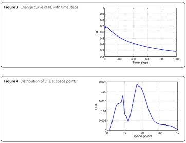
Figure 3Change curve of RE with time steps

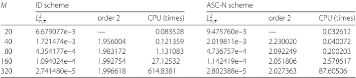
Figure 4Distribution of DTE at space points

Then we will analyze the distribution of the difference total energy (DTE) at space grid points. The definition of DTE is as follows:

DTE(j) = 1 2

M

i=1

u(xi,tj) –uij

2

.

From Fig.3, the RE of ASC-N scheme is less than 0.75. The RE is a little big in the first few steps and decreases rapidly with the time step. Therefore, we can know that the ASC-N scheme of the time fractional sub-diffusion equation is stable.

The DTE of ASC-N scheme is between 0 and 0.025 from Fig.4. It can also demonstrate that the ASC-N scheme is very close to the exact solution. The DTE appears to fluctuate near the grids 8, 16, 24, 32. And its maximum values appear near the grids 8 and 16. The grids 8, 16, 24, 32 are the “inter boundary point” of the ASC-N scheme. The four kinds of Saul’yev scheme are alternatively applied at the “inter boundary point”. The classic C-N scheme is applied at the inter point for the ASN scheme. The truncation error of the C-N scheme is better than the four kinds of Saul’yev scheme. So the DTE of “inter boundary point” is little bigger than the DTE of inter point. The result of Fig.4is consistent with theoretical analysis.

The next example will be performed to illustrate the computational efficiency and con-vergence rate of the ASC-N scheme. Denote

L2_h,τ =

M

i=1

u(xi,tM) –uMi

2

, order 1 =log₂ L 2

τ

L2τ/2

, order 2 =log₂ L 2

h

L2_h/2.

Table 2 The numerical errors and convergence orders in temporal direction (h= 1/80)

α N ID scheme ASC-N scheme

L2_h,τ order 1 CPU (times) L2_h,τ order 1 CPU (times)

0.8 400 1.553456e–4 — 0.592518 1.615210e–4 — 0.121606

800 6.820719e–5 1.187486 1.572824 6.961018e–5 1.214352 0.272843

1600 2.980843e–5 1.194203 4.995801 3.013909e–5 1.207662 0.757238

3200 1.299478e–5 1.197787 17.68847 1.307457e–5 1.204872 2.459121

6400 5.657158e–6 1.199783 67.09086 5.676690e–6 1.203642 8.867395

0.5 400 3.023084e–5 — 0.614962 3.901743e–5 — 0.133529

800 1.072534e–5 1.494996 1.557829 1.244259e–5 1.648831 0.260445

1600 3.788676e–6 1.501258 4.963961 4.138894e–6 1.587970 0.741085

3200 1.332788e–6 1.507246 17.56794 1.406616e–6 1.557016 2.419346

6400 4.666755e–7 1.513955 66.60791 4.827127e–7 1.542992 8.741754

0.4 400 1.399030e–5 — 0.621470 2.705434e–5 — 0.136365

800 4.601493e–6 1.604253 1.568314 7.015947e–6 1.947150 0.266416

1600 1.501415e–6 1.615778 4.983283 1.980694e–6 1.824631 0.761807

3200 4.849224e–7 1.630497 17.93907 5.825449e–7 1.765565 2.535364

6400 1.543647e–7 1.651411 67.22779 1.746222e–7 1.738132 9.100791

Table 3 The numerical errors and convergence orders in spatial direction (α= 0.5,τ=h2)

M ID scheme ASC-N scheme

L2_h,τ order 2 CPU (times) L2_h,τ order 2 CPU (times)

20 6.679077e–3 — 0.083528 9.475760e–3 — 0.032612

40 1.721474e–3 1.956004 0.121359 2.019811e–3 2.230020 0.040072

80 4.354177e–4 1.983172 1.131083 4.736757e–4 2.092249 0.200203

160 1.094024e–4 1.992754 27.12532 1.142419e–4 2.051806 2.578617

320 2.741480e–5 1.996618 614.8381 2.802388e–5 2.027363 87.60506

using the same machine withα= 0.8, 0.5, 0.4, respectively. From Table2, we can see that the numerical accuracy in temporal direction is order 2 –αfor these three cases.

Secondly, we compute the numerical accuracy in spatial direction. TakeM= 20, 40, 80, 160, 320 for the ID and ASC-N schemes, and letτ =h2_(N=M2_{/10). From Table3, we can}

see that the numerical accuracy in spatial direction is second order for the ID and ASC-N schemes. The same convergence orders of spatial and temporal direction are obtained for both of them.

In terms of computational efficiency, the CPU times of the ASC-N have big advantage compared with the ID scheme. From Tables2and3, we know that the parallel computing advantages of the ASC-N scheme will be more obvious with the increase of the number of time layers or space lattice points. Comparing with the ID scheme the CPU times of the ASC-N scheme can save near 90%. Comprehensively considering the computational efficiency and computational accuracy, the ASC-N scheme can be more effective to solve the time fractional sub-diffusion equation. When the long time course is calculated, the parallel computing advantages of the ASC-N scheme will be more evident.

6 Conclusion

The ASC-N scheme has ideal computing accuracy and computing efficiency. The par-allel computing advantages of the ASC-N scheme will be more obvious for the long time course or the high dimensional fractional diffusion equation.

Funding

The work was supported by the National Natural Science Foundation of China (Grant No. 11371135) and the Fundamental Research Funds for the Central Universities (Grant No. 2018MS168).

Competing interests

The authors declare that they have no competing interests.

Authors’ contributions

They all read and approved the final version of the manuscript.

Publisher’s Note

Springer Nature remains neutral with regard to jurisdictional claims in published maps and institutional affiliations.

Received: 9 April 2018 Accepted: 8 August 2018

References

1. Diethelm, K.: The Analysis of Fraction Differential Equations. Springer, Berlin (2010) 2. Uchaikin, V.V.: Fractional Derivatives for Physicists and Engineers, vol. II. Springer, Berlin (2013)

3. Agrawal, O.P.: Solution for a fractional diffusion-wave equation defined in a boundary domain. J. Nonlinear Dyn.29, 145–155 (2002)

4. Bao, J.D.: Introduction to Abnormal Statistical Dynamics. Science Press, Beijing (2012) (in Chinese)

5. Yang, X.J., Machado, J.A.T., Baleanu, D.: Anomalous diffusion models with general fractional derivatives within the kernels of the extended Mittag-Leffler type functions. Rom. Rep. Phys.69, 151 (2017)

6. Chen, W., Sun, H.G., Li, X.C.: Fractional Derivative Modeling of Mechanics and Engineering Problems. Science Press, Beijing (2010) (in Chinese)

7. Yang, X.J., Machado, J.A.T.: A new fractional operator of variable order: application in the description of anomalous diffusion. Phys. A, Stat. Mech. Appl.481, 276–283 (2017)

8. Guo, B.L., Pu, X.K., Huang, F.H.: Fractional Partial Differential Equations and Their Numerical Solutions. Science Press, Beijing (2011) (in Chinese)

9. Sun, Z.Z., Gao, G.H.: Finite Difference Method for Fractional Differential Equations. Science Press, Beijing (2015) (in Chinese)

10. Liu, F.W., Zhuang, P.H., Liu, Q.X.: Numerical Methods and Applications of Fractional Partial Differential Equations. Science Press, Beijing (2015) (in Chinese)

11. Zhuang, P., Liu, F.: Implicit difference approximation for the time fractional diffusion equation. J. Appl. Math. Comput.

22(3), 87–99 (2006)

12. Tadjeran, C., Meerschaert, M.M., Scheffler, H.P.: A second-order accurate numerical approximation for the fraction diffusion equation. J. Comput. Phys.213(1), 205–213 (2006)

13. Chen, C.M., Liu, F.W., Turner, I., et al.: Numerical schemes and multivariate extrapolation of a two-dimensional anomalous sub-diffusion equation. Numer. Algorithms54(1), 1–21 (2010)

14. Zhang, P., Pu, H.: The error analysis of Crank–Nicolson-type difference scheme for fractional subdiffusion equation with spatially variable coefficient. Bound. Value Probl.2017, 15 (2017)

15. Baleanu, D., Jajarmi, A., Asad, J.H., Blaszczyk, T.: The motion of a bead sliding on a wire in fractional sense. Acta Phys. Pol.131(6), 1561–1564 (2017)

16. Jajarmi, A., Hajipour, M., Mohammadzadeh, E., Baleanu, D.: A new approach for the nonlinear fractional optimal control problems with external persistent disturbances. J. Franklin Inst.355, 3938–3967 (2018)

17. Hajipour, M., Jajarmi, A., Baleanu, D.: An efficient non-standard finite difference scheme for a class of fractional chaotic systems. J. Comput. Nonlinear Dyn.13, 021013 (2018)

18. Wang, H., Treena, S.B.: A fast finite difference method for two-dimensional space-fractional diffusion equations. SIAM J. Sci. Comput.34(5), A2444–A2458 (2012)

19. Wang, H., Du, N.: A fast finite difference method for three-dimensional time-dependent space-fractional diffusion equations and its efficient implementation. J. Comput. Phys.253(45), 50–63 (2013)

20. Gao, G.H., Sun, Z.Z.: A compact finite difference scheme for the fractional sub-diffusion equations. J. Comput. Phys.

230(3), 586–595 (2011)

21. Gao, G.H., Sun, Z.Z.: Two difference schemes for solving the one-dimensional time distributed-order fractional wave equations. Numer. Algorithms74, 675–697 (2017)

22. Yaseen, M., Abbas, M., Nazir, T., Baleanu, D.: A finite difference scheme based on cubic trigonometric B-splines for a time fractional diffusion-wave equation. Adv. Differ. Equ.2017, 274 (2017)

23. Zaky, M.A., Baleanu, D., Alzaidy, J.F., Hashemizadeh, E.: Operational matrix approach for solving the variable-order nonlinear Galilei invariant advection-diffusion equation. Adv. Differ. Equ.2018, 102 (2018)

24. Zhang, B.L., Yuan, G.X., Liu, X.P., Chen, J.: Parallel Finite Difference Methods for Partial Differential Equations. Science Press, Beijing (1994) (in Chinese)

25. Zhang, B.L., Gu, T.X., Mo, Z.Y.: Principles and Methods of Numerical Parallel Computation. National Defence Industry Press, Beijing (1999) (in Chinese)

27. Petter, B., Mitchell, L.: Parallel Solution of Partial Differential Equations. Springer, New York (2000)

28. Yuan, G.W., Yue, J.Y., Sheng, Z.Q., et al.: The computational method for nonlinear parabolic equation. Sci. Sin., Math.43, 235–248 (2013) (in Chinese)

29. Yuan, G.W., Sheng, Z.Q., Hang, X.D., et al.: The Calculation Method of Diffusion Equation. Science Press, Beijing (2015) (in Chinese)

30. Wang, W.Q.: A class of alternating group method of Burgers’ equation. Appl. Math. Mech.25(2), 236–244 (2004) 31. Wu, L.F., Yang, X.Z., Zhang, F.: A kind of difference method with intrinsic parallelism for nonlinear Leland equation.

J. Numer. Methods Comput. Appl.35(1), 69–80 (2014) (in Chinese)

32. Diethelm, K.: An efficient parallel algorithm for the numerical solution of fractional differential equations. Fract. Calc. Appl. Anal.14(3), 475–490 (2011)

33. Gong, C.Y., Bao, W.M., Tang, G.J.: A parallel algorithm for the Riesz fraction reaction-diffusion equation with explicit finite difference method. Fract. Calc. Appl. Anal.16(3), 654–669 (2013)

34. Gong, C.Y., Bao, W.M., Tang, G.J., et al.: An efficient parallel solution for Caputo fractional reaction-diffusion equation. J. Supercomput.68, 1521–1537 (2014)

35. Wang, Q.L., Liu, J., Gong, C.Y., et al.: An efficient parallel algorithm for Caputo fractional reaction-diffusion equation with implicit finite-difference method. Adv. Differ. Equ.2016, 207 (2016)

36. Sweilam, N.H., Moharram, H., Moniem, N.K.A., Ahmed, S.: A parallel Crank–Nicolson finite difference method for time-fractional parabolic equation. J. Numer. Math.22(4), 363–382 (2014)

37. Chi, X.B., Wang, Y.W., Wang, Y., Liu, F.: Parallel Computing and Implementation Technology. Science Press, Beijing (2015) (in Chinese)