Digital Commons@Georgia Southern
Electronic Theses and Dissertations Graduate Studies, Jack N. Averitt College of
Fall 2018
Multiclass Classification Using Support Vector Machines
Duleep Prasanna W. Rathgamage DonFollow this and additional works at: https://digitalcommons.georgiasouthern.edu/etd
Part of the Artificial Intelligence and Robotics Commons, Other Applied Mathematics Commons, and the Other Statistics and Probability Commons
Recommended Citation
Rathgamage Don, Duleep Prasanna W., "Multiclass Classification Using Support Vector Machines" (2018). Electronic Theses and Dissertations. 1845.
https://digitalcommons.georgiasouthern.edu/etd/1845
This thesis (open access) is brought to you for free and open access by the Graduate Studies, Jack N. Averitt College of at Digital Commons@Georgia Southern. It has been accepted for inclusion in Electronic Theses and Dissertations by an authorized administrator of Digital Commons@Georgia Southern. For more information, please contact [email protected].
by
DULEEP RATHGAMAGE DON (Under the Direction of Ionut Iacob)
ABSTRACT
In this thesis we discuss different SVM methods for multiclass classification and introduce the Divide and Conquer Support Vector Machine (DCSVM) algorithm which relies on data sparsity in high dimensional space and performs a smart partitioning of the whole train-ing data set into disjoint subsets that are easily separable. A strain-ingle prediction performed between two partitions eliminates one or more classes in a single partition, leaving only a reduced number of candidate classes for subsequent steps. The algorithm continues recur-sively, reducing the number of classes at each step, until a final binary decision is made between the last two classes left in the process. In the best case scenario, our algorithm makes a final decision betweenk classes inO(log2k)decision steps and in the worst case scenario DCSVM makes a final decision ink−1steps.
INDEX WORDS: Statistical learning, Classification, Curse of dimensionality, Support Vector Machine, Kernel trick
by
DULEEP RATHGAMAGE DON
B.S., The Open University of Sri Lanka, Sri Lanka, 2008
A Thesis Submitted to the Graduate Faculty of Georgia Southern University in Partial Fulfillment of the Requirements for the Degree
MASTER OF SCIENCE STATESBORO, GEORGIA
DULEEP RATHGAMAGE DON All Rights Reserved
MULTICLASS CLASSIFICATION USING SUPPORT VECTOR MACHINES by
DULEEP RATHGAMAGE DON
Major Professor: Ionut Iacob
Committee: Mehdi Allahyari
Stephen Carden Goran Lesaja
Electronic Version Approved: December 2018
DEDICATION
I dedicate this thesis to my beloved wife Kasuni Nanayakkara, Ph.D. for nursing me with affections and guiding me to the success in my life.
ACKNOWLEDGMENTS
I am grateful to my graduate adviser Dr. Huwa Wang and my thesis adviser Dr. Ionut Iacob for their valuable academic and research guidance and placing their trust in my abilities for all my achievements at Georgia Southern University. I am also grateful to all my professors at Georgia Southern University with special thanks to Dr. Saeed Nasseh, Dr. Stephen Carden and Dr. Goran Lesaja who made an enthusiasm in my graduate studies. My forever interested, Sri Lankan professors V. P. S. Perera, W. Ramasinghe, and W. B. Daundasekara: they were always a part of my higher education and professional development. I appreciate your support in my past endeavors. A special gratitude goes to Ms. Kathleen Hutcheson: as my boss she made my 7thteaching job very pleasant. At last but by no means least, I would like to be thankful to all the graduate students and staff at the Department of Mathematical Sciences. Thanks for all your encouragement!
TABLE OF CONTENTS Page ACKNOWLEDGMENTS . . . 3 LIST OF TABLES . . . 6 LIST OF FIGURES . . . 7 LIST OF SYMBOLS . . . 9 CHAPTER 1 Introduction . . . 10
2 Statistical Learning Theory . . . 12
2.1 Vapnik Chernonkis (VC) Dimension . . . 12
2.2 Structural Risk Minimization . . . 14
3 Introduction to Support Vector Machine . . . 16
3.1 Hard Margin Support Vector Machine . . . 16
3.2 Soft Margin Support Vector Machine . . . 20
3.3 Kernel Trick . . . 23
3.4 Implementation . . . 26
3.4.1 Selection of Parameters . . . 28
3.4.2 Training . . . 29
3.4.3 Evaluation of Performance . . . 30
4 Multiclass Support Vector Machines . . . 36
4.1 One Versus Rest Support Vector Machine . . . 36
4.2 One Vs One Support Vector Machine . . . 37
30 31
4.3 Directed Acyclic Graph Support Vector Machine . . . 39
5 Fast Multiclass Classification . . . 41
5.1 Curse of Dimensionality . . . 41
5.2 Divide and Conquer Support Vector Machine (DCSVM) . . . 42
5.2.1 Architecture of DCSVM . . . 44
5.2.2 A Working Example . . . 52
5.3 Experiments . . . 54
5.4 Results . . . 55
5.4.1 Comparison of Accuracy . . . 56
5.4.2 Prediction Performance Comparison . . . 56
5.4.3 DCSVM Performance Fine Tuning . . . 57
6 Conclusion . . . 64
65 68 REFERENCES . . . . APPENDIX A DetailsoftheDatasets .. . . ... . . . APPENDIX B RCodesoftheExperiments . . . ... . . . 69
B.1 Example 3.3 and proceedings . . . 69
B.2 Precessing datasets . . . 70
B.3 Building Multiclass SVMs . . . 76
B.4 Experimental Results: Section 5.4.1 and 5.4.2 . . . 91
B.5 Collecting Split Percentages . . . 99
LIST OF TABLES
Table Page
3.1 Some common kernels . . . 26
5.1 svmoptimality measures forglassdataset and the initialAll-Predictions
table . . . 53 5.2 Optimality measures in the second step of creating the decision tree in
Figure 5.3 (b) . . . 55 5.3 Prediction accuracies for different split thresholds . . . 60
5.4 DCSVM: average number of steps per decision for different split
thresholds . . . 61
5.5 DCSVM: average support vectors per decision for different split
thresholds . . . 62
LIST OF FIGURES
Figure Page
2.1 Block diagram of the basic model of a learning machine . . . 12
2.2 Shattering of linear classifier in 2-dimensional space . . . 13
2.3 Structural risk minimization of a learning machine . . . 15
3.1 Binary classification problem: building up support vector machine . . . 16
3.2 Hard margin support vector machine . . . 17
3.3 Soft margin support vector machine . . . 20
3.4 Trade-off between maximum margin and minimum training error . . . 21
3.5 Nonlinear classification . . . 23
3.6 Scatter plot of synthetic1 . . . 27
3.7 Performance of SVM - grid search of learning parameters . . . 29
3.8 SVM classification plot of synthetic1 . . . 30
3.9 The format of confusion matrix for synthetic1 . . . 31
3.10 Receiver Operating Characteristic (ROC) curve for synthetic1 . . . 33
4.1 One versus rest method: classification between 3 classes . . . 36
4.2 One against one method: classification between 3 classes . . . 38
4.3 Input space of a 4 class problem . . . 39
4.4 Directed acyclic graph support vector machine: 4 class problem . . . . 39
5.1 VC confidence against VC dimension/number of training data . . . 42
30 31 32 35
5.2 Seperation of classess 1 and 2 by a linear SVM classifier . . . 44
5.3 Prediction plan of glass for threshold = 0.05 . . . 46
5.4 DCSVM decision tree with (a) the decision process forglassdataset (b) the classification of an unseen instance . . . 54
5.5 Average prediction accuracy (%) . . . 56
5.6 Average number of support vectors . . . 57
5.7 Average number of steps . . . 58
5.8 Average prediction time (sec) . . . 58
5.9 Accuracy and the average number of prediction steps for different likelihood thresholds . . . 59
LIST OF SYMBOLS
R Real numbers
Rn n-dimensional Euclidean space
H Hilbert Space
sign(x) Sign function of x
dim(X) Dimension of vector space X
SV Set of support vectors
x Vector x
xT Transpose of vector x
n r
Set of all r-combinations of n elements
k·k Vector norm
Pn
i=1 Summation operator over i from 1 to n
5 Vector differential operator
∂
∂x Differential operator with respect to x
R
x,x Double integral operator with respect to x
<·,·> Inner product
svmi,j SVM binary classifier
Ci,j(l, i) Class predictions likelihood of SVM for label l
Pi,j(θ) Purity index of SVM for accuracy thresholdθ
CHAPTER 1 INTRODUCTION
Support Vector Machines (SVMs) belong to the class of supervised learning methods in machine learning and artificial intelligence. They learn from data and recognize patterns which are useful for classification and regression. The SVMs are widely used as a reliable tool for data mining, pattern recognition, and predictive analytics in medicine, engineering, and business.
In the 1960’s the statistical learning theory was mostly developed for learning algo-rithms of nonlinear functions through the seminal work by Vapnik and Chervonenkis [12]. The statistical learning theory deals with the following fundamental problems about learn-ing from data: what conditions help a model learn from examples? and how does the performance measured on selected of examples lead to the bounds on generalization in (2.3)? There is still ongoing research in this area and the conditions for theories to be valid are almost impossible to check for most practical problems [24]. The same researchers pro-posed the restoration of linear separability methods, with additional ingredients intended to improve generalization, with the name of Support Vectors Machines (SVM).
In 1992, Bernhard Boser, Isabelle Guyon, and Vladimir Vapnik developed a method for nonlinear classification by introducing the kernel trick to maximum-margin SVM [9]. A later extension of SVM was found with soft margin classification contributing to doc-ument classification where preference solution was to better separate the bulk of the data while ignoring a few outliers. Further, multiclass SVMs were developed to handle a mul-ticlass classification problem by decomposing the original problem into a series of binary problems so that the standard SVM could be directly applied to each problem. The mul-ticlass classification with SVM is still an ongoing research problem (see, for example, [13, 18, 19, 21] for some recent work). In this study, we especially focus on a novel SVM designed for the classification of multiclass and high dimensional datasets [24].
Due to recent technological advances, a large amount of high-throughput data can be collected simultaneously and at relatively low-cost [25]. Classification of such data raises new challenges, for instance, deterioration in the accuracy of learning algorithms with the dimension of data. The reason is that the data becomes sparse at high dimensions making training of the learning algorithms problematic due to large regularization error or computational complexity. These phenomena referred to as the curse of dimensionality set the motivation for our research [27].
We observed that a binary SVM decision boundary might separate more than two classes of data in multiclass settings (Fig 5.2). The observation can be repeated until all the classes are eliminated. This concept is even more persistent when the data becomes sparse as their dimension increases. Our method utilizes a decision tree approach to investigate this property for a given dataset. The first step is similar to One-Vs-One method where a pool of SVM classifiers are built considering any pair of classes. We grade them according to their impurity, balance, and score (see the definitions 5.3 and 5.4). The best classifier is selected to be the top node of the decision tree (Fig 5.4). Then the selection procedure is repeated on a reduced pool of SVM to figure out the other nodes of the decision tree until all the classes are separated [24].
The performance of DCSVM is tested against classifying some real datasets found in the UCI machine learning repository. We implemented tenfold cross-validation and aver-aged the results to compare the DCSVM with the classic One-Vs-One method in terms of the prediction accuracy, number of support vectors, number of binary decisions, and predic-tion time. The DCSVM has several advantages over the One-Vs-One method including but not limited to less predicting time, and less computational complexity while maintaining the same prediction accuracy.
CHAPTER 2
STATISTICAL LEARNING THEORY Let us consider the basic model of a learning machine.
Figure 2.1: Block diagram of the basic model of a learning machine
Suppose we have a learning machine whose task is to learn the mappingxi 7→ yi for i= 1, . . . , nwherexi ∈X, a m dimensional vector andyi ∈Y ={−1,1}, a set of labels.
The machine is actually defined by a set of possible mappings X 7→ f(X, α), where the function is governed by an adjustable parameter α referred to its representational power which is a measure of the complexity of the learning machine. There is an important set of bounds controlling the relationship between the performance of a learning machine and it’s representational power [8]. The usual trade-off in this case is that more power results in over-fitting while the less power might end up in under-fitting.
2.1 VAPNIKCHERNONKIS (VC) DIMENSION
In order to characterize the representational power of a learning task assigned to a machine or its hypothesis class, we consider the VC dimension.
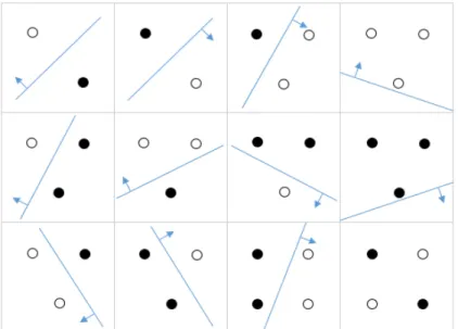
Definition 2.1. Given that A is a set and C is a collection of sets. C is said to shatter A if for each a⊂A, there exists c∈C such that,
Definition 2.2. VC dimension of a hypothesis class is the maximum number of data points that can be arranged so that the learning machine can shatter them.
Consider the following hypothesis class. i.e., linear classifier in 2-dimensional space.
Figure 2.2: Shattering of linear classifier in 2-dimensional space
It is clear that the VC dimension of this particular hypothesis class is three as the given configuration of four data points in the last block of Figure 2.2 cannot be shattered.
Theorem 2.1. (proof is omitted) Consider some set of m points inRn. Choose any one of the points as origin. Then the m points can be shattered by oriented hyperplanes if and only if the position vectors of the remaining points are linearly independent.
Corollary 2.2. The VC dimension of the set of oriented hyperplanes inRnisn+ 1.
Proof. We can always choosen+1points, and then choose one of the points as origin, such that the position vectors of the remainingn points are linearly independent, but can never choosen+ 2such points (since non+ 1vectors inRncan be linearly independent).
2.2 STRUCTURALRISKMINIMIZATION
It is assumed that there exists some unknown cumulative probability distributionP (X, Y)
from which the data are drawn i.e., the data assumed to be independently drawn and iden-tically distributed (iid). The expectation of the test error for a trained machine is therefore (using Lebesgue integration):
R(f) = 1 2
Z
|Y −f(X, θ)|dP (X, Y) (2.1)
Where,R(f)is called the expected risk or true risk. Given that the number of training instances isn, the empirical riskRemp(f)is defined to be the measured mean error on the
training set. Remp(f) = 1 2n n X i=1 |Y −f(X, θ)| (2.2)
The quantity 12|Y −f(X, θ)| is called the loss. For this case, it can only take the values 0 and 1. Now choose some η such that0 ≤ η ≤ 1. Then for losses taking these values, with the probability1−ηthe following bounds hold [8].
R(f) = Remp(f) +
r
h(log (2n/h) + 1)−log (η/4)
n (2.3)
Where h is VC dimension. The second term on the right hand side is called VC
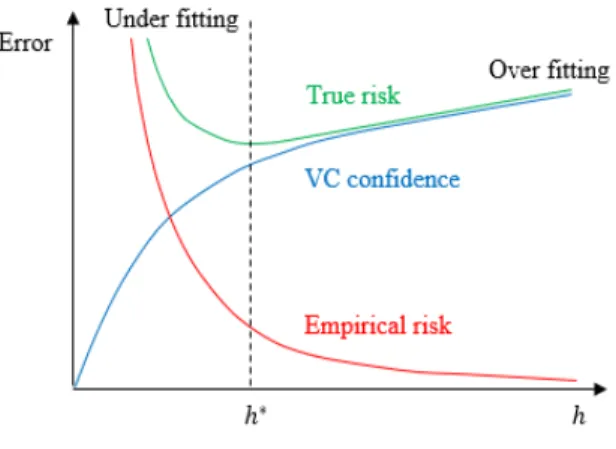
confidence. If we know h, we can easily compute the right hand side of (2.3). Thus we consider several different learning machines, for sufficiently small η. Then choosing the machine that minimizes the right hand side of (2.3), we find the machine which gives the lowest upper bound on the true risk as shown in Figure 2.3. This gives a principle method for choosing a learning machine for a given task, and it is the essential idea of Structural Risk Minimization (SRM) [8].
Figure 2.3: Structural risk minimization of a learning machine
Also notice that the VC confidence of (2.3) may be ignored for very large n. In prac-tice, we will not have infinitely many instances in the training dataset. If h is too large with respect to n, then there is a risk of over-fitting the training data. Hence, the SRM plays an important role in implementing supervised learning machines. The SRM is an inductive principle for model selection from finite training datasets. The goal of this principle is to govern the generalization error of the learning machine by limiting the flexibility of the set of decision functions, measured by the VC dimension. Instead of utilizing a decision functionf by minimizing the training error on a selected data set,f is selected to minimize an upper bound on the test error given by (2.3) as outlined below.
1. Using a prior knowledge of the domain, choose a class of functions and divide it into a hierarchy of nested subsets in order of increasing complexity.
2. Perform empirical risk minimization on each subset (this is essentially parameter selection).
3. Select the model (h∗ ) in the series whose sum of empirical risk and VC confidence
CHAPTER 3
INTRODUCTION TO SUPPORT VECTOR MACHINE 3.1 HARDMARGIN SUPPORTVECTOR MACHINE
The simplest version of SVM is the learning machine that classify m-dimensional linearly separable data into two classes C1and C2depending on the labels yi.
Definition 3.1. A set of m-dimensional binary class data is linearly separable if there exists at least one m−1 dimensional vector space called hyperplane with all the data points of C1 on one side of the hyperplane and all the data points of C2 on the other side.
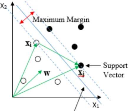
The gap between the linearly separable data is known as margin. The hyperplane is made in such a way that the margin is maximized. Suppose that we randomly select some vectorsxi for the training set. Our goal is to find the optimal hyperplane that classifies all
the training data into two classes. Figure 3.1 shows a 2-dimensional feature space, however the following method can be applied to the general case.
Figure 3.1: Binary classification problem: building up support vector machine
Suppose a given xi is on the hyperplane. w is a normal vector called weight which
of the hyperplane [10]. Then the equation of the hyperplane iswTxi +b= 0 as it linear.
Then the SVM is a learning machine with a decision rule of the form:
f(xi, α) =sign(wTxi+b) (3.1)
Suppose for an arbitraryxiwe have
f(xi, α) =wTxi+b >1, if xi ∈C1
=wTxi+b <−1, if xi ∈C2;
(3.2)
Now for eachxiandwwe chooseyi ∈Y, set of class labels such that
yi =
1, if xi ∈C1
−1, if xi ∈C2 Both (3.2) relationships imply that
yi(wTxi+b)−1≥0; w∈Rn, b∈R (3.3)
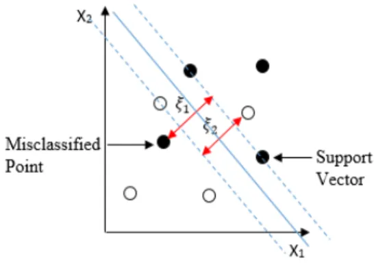
Definition 3.2. Support vectors are the data points of the classes C1 and C2 that are at the boundary of the maximum margin as shown in Figure 3.2.
To find the width of the margin, consider thexi andxj shown in Figure 3.2
The width of the margin is(xj −xi)w/kwk
By (3.2),
The width of the margin= 2
kwk (3.4)
Our goal is to maximize the margin, i.e., to minimizekwk. Now the quadratic programing problem is
min w∈Rm 1 2kwk 2 subject to (3.3)
The solution to the above problem is a global minimum satisfying the Karush−Kuhn−Tucker (KKT) conditions.
Definition 3.3. KKT conditions for the optimization problem with the objective function
f :Rn 7→
Rand constraint functionsgj : Rn 7→Randhk : Rn 7→ Rsuch thatf,g, andh
are continuously differentiable at a local optimumx∗ for constantsαj (j = 1,...,m) andβk
(k = 1,...,l) are given below.
Condition 1 (Stationarity) For maximizing f(x): 5f(x∗) =Pm j=1αj5gj(x ∗) +Pl k=1βk5hk(x ∗) For minimizing f(x): − 5f(x∗) = Pm j=1αj5gj(x ∗) +Pl k=1βk5hk(x ∗)
Condition 2 (Primal Feasibility)
gj(x∗)≤0for j = 1,...,m andhk(x∗) = 0for k = 1,...,l Condition 3 (Dual Feasibility)
αj ≥0for j = 1,...,m
Condition 4 (Complementary Slackness)
αjgj(x∗) = 0for j = 1,...,m
To apply the KKT conditions, it is customary to write our optimization problem in the form of following auxiliary function (similar to Lagrangian) using the primal feasibility.
Lp(w, b, αj) = 1 2 kwk 2 − n X j=1 αj[yj(wTxj+b)−1] (3.5)
To find the solution, first we minimize (3.5) with respect to w and b and subject to (3.3). Hence this optimization is known as the primal problem.
Let us write (3.5) in the following way.
Lp(w, b, αj) = 1 2 kwk 2 − n X j=1 αjyjwTxj − n X j=1 αjyjb+ n X j=1 αj
Considering the stationarity;∂Lp/∂b = 0and∂Lp/∂w= 0, it follows that: n X j=1 αjyj = 0 (3.6) w= n X j=1 αjyjxj (3.7)
To obtain the minimum solution of the primal problem, we substitute (3.6) and (3.7) in (3.5) with new indexing to obtain the dual problem (3.8).
Ld(αi) = n X i=1 αi− 1 2 n X i=1 n X j=1 αiαjyiyj(xixj) (3.8)
Considering dual feasibility, we can maximize (3.8) with respect to αi. and subject
to (3.6) Assume the solution of the dual problem is found by using Sequential Minimal Optimization [28] which is commonly used in practice. An appropriate quadratic program-ing package can also be used in this case if the dual problem is set for a minimization. The corresponding maximizers are considered to be the non-zero Lagrange multipliersα∗
associated with the support vectors.
Ifxj is a support vector, then from (3.7)
w= X j∈SV
α∗jyjxj (3.9)
After the dual problem is solved, the bias is calculated by using (3.10) [22]
b = 1 #SV X j∈SV yj −wTxj ! (3.10)
By substituting (3.9) and calculated (3.10) in (3.1), we modify our decision rule on testing data xi as in (3.11). This is the essential procedure of training the hard margin
SVM. wandαare called SVM classification parameters. Note that the hard margin SVM is suitable for linearly separable data [10].
f(xi, α) =sign X j∈SV α∗jyj(xjxi) +b ! (3.11)
3.2 SOFTMARGINSUPPORTVECTOR MACHINE
Figure 3.3: Soft margin support vector machine
If the data is nearly linearly separable (e.g., due to noise), the condition for the optimal hyper-plane can be relaxed by including an extra term: slack variableξias shown in Figure
3.3. This idea will result in an efficient classifier know as soft margin SVM. From (3.3)
Then the quadratic programming problem becomes; minw∈Rm 1 2 kwk 2 +C n X j=1 ξj (3.13) subject to (3.12)
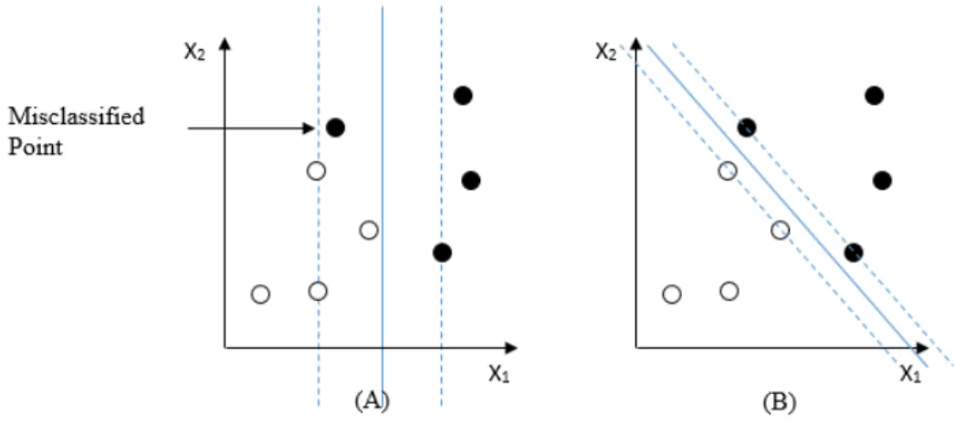
Here, C is a regularization parameter called the cost of the SVM that controls the trade-off between maximizing the margin and minimizing the training error by imposing a penalty on the objective function for misclassification. Small C tends to emphasize the margin while ignoring the outliers in the training data as Figure 3.4 (A), while largeCmay tend to over fit the training data as Figure 3.4 (B).
Figure 3.4: Trade-off between maximum margin and minimum training error
As in the hard margin case, using KKT conditions, the primal form of (3.13) can be expressed as, Lp(w, b, ξj, αj, λj) = 1 2kwk 2 +C n X j=1 ξj− n X j=1 αj[yi(wTxj+b)−1 +ξj]− n X j=1 λjξj (3.14) subject to (3.12)
We write (3.14) in the following way
Lp ≡ 1 2kwk 2 +C n X j=1 ξj−wT n X j=1 αjyjxj−b n X j=1 αjyj + n X j=1 αj − n X j=1 αjξj − n X j=1 λjξj
considering the stationarity;∂Lp/∂w= 0,∂Lp/∂b= 0, and∂Lp/∂xij = 0, it follows that: w= n X j=1 αjyjxj (3.15) n X j=1 αjyj = 0 (3.16) C−αj −λj = 0 (3.17)
respectively. Substitute (3.15), (3.16), and (3.17) in (3.14), to obtain the dual problem which is similar to (3.8) and subject to (3.16) and (3.17). The only significant difference between the two dual problems is the soft margin dual problem has a Lagrange multiplier bounded above.
It is clear thatλj is a Lagrange multiplier and hence nonnegative. Ifλj = 0, then from
(3.17) it follows that αj = C. Ifλj > 0, then from (3.17) it follows thatαj < C. Hence
the dual problem for (3.14) that needs to be maximized with respect to αj and subject to 0≤αj ≤Cis given below. Ld(αj) = n X i=1 αi− 1 2 n X i=1 n X j=1 αiαjyiyj(xixj) (3.18)
The solution to (3.18) can be obtained by using the same techniques used to solve (3.8). Then the decision rule of the soft margin SVM is similar to (3.11).
To find the type of support vectors of the soft margin SVM, we consider the comple-mentary slackness for the optimization problem as follows.
αj[yj(wTxj +b)−1 +ξj] = 0 (3.19)
λjξj = 0 (3.20)
It follows that for a support vectorαj 6= 0. Then from (3.19) we observe the following.
There are two types of support vectors associated with the training of soft margin SVM. If λj >0, then from (3.20)ξj = 0and from (3.21) it follows that this data point is
at the boundary of the margin. From (3.19) we haveαj < C. Ifλj = 0, then from (3.20) ξj > 0and from (3.21) it follows that this data point is over the margin. From (3.17) we
have αj = C. The choice of an appropriate value forC is an essential part of tuning an
SVM and is discussed in chapter 3.4.
3.3 KERNELTRICK
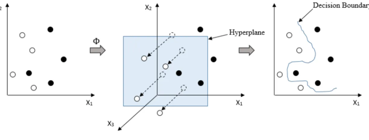
Let us consider the problem with hard margin. If the data is not linearly separable, the optimization of (3.8) can be performed on a higher dimensional vector space. In this case, the data is mapped from input-space to feature-space by a mapping Φ and the optimal separating hyperplane is found. Then the separation is mapped back down to input-space, where it results in a non-linear decision boundary as shown in Figure 3.5.
Figure 3.5: Nonlinear classification
LetU andV be vector spaces such that dim(V)>dim(U) andΦbe a function given byΦ: U →V. Forxi, xj ∈ U(input space), from (3.8) the corresponding optimization in
V(feature space) is, max n X i=1 αi− 1 2 n X i=1 n X j=1 αiαjyiyjΦ(xi)Φ(xj) (3.22)
with respect to αi and subject to (3.6). Calculation of Φ(xi)Φ(xj)is very expensive
in both computation and memory consumption as the dimension of feature space could be very large or even infinity. Kernel trick allows us to perform the above task without actually transforming the training data into the high dimensional feature space.
Example 3.1. Let x and y be two dimensional vectors such that x ≡ (x1, x2) and y ≡
(y1, y2)andΦbe a transformation such thatΦ :R2 7→R3given byΦ(s, t) = (s2, t2, √
2st);
s, t ∈R. We can show that the dot product ofxandycan be obtained using a certain func-tionkknow as the kernel function.
<Φ(x),Φ(y)>= (x21, x22,√2x1x2)(y12, y22, √ 2y1y2)T = ((x1, x2)(y1, y2)T)2 =<x,y>2 =k(x,y)
Note that not all kernel functions can perform a sort of calculation in the example above. A kernel function that legitimately behaves as in the example above is called a Mercer kernelkintroduced in Mercer’s theorem.
Theorem 3.2. Mercer’s Theorem (Proof is omitted) Let X∈ Rn. For any symmetric con-tinuous function k: X×X7→Rsuch that k∈L2(X) (square integrable in X×X) satisfying,
Z
X,X
f(x0)k(x, x)f(x)dxdx0 ≥0 (3.23)
for all f∈L2(X)
There exist functionsΦi: X7→ Hand constantsλi ≥0 such that
k(x, x0) = ∞ X i=1 λiΦi(x)Φi(x0) (3.24) for all x, x’∈X
Definition 3.4. The kernel trick is the relationship in (3.25) where k is a Mercer kernel. It can be used to avoid the mapping needed for linear learning algorithms to learn a non-linear function or decision boundary by implicitly calculating the inner products between the feature vectors.
k(xi,xj) = Φ(xi).Φ(xj) (3.25)
It is clear that (3.22) will result in the following decision rule.
f(xi, α) =sign X j∈sv α∗jyjΦ(xj)Φ(xi) +b ! (3.26)
To apply the kernel trick in the nonlinear decision rule, we substitute (3.25) in (3.26)
f(xi, α) =sign X j∈sv α∗jyjk(xi,xj) +b ! (3.27)
There are several different kernel functions used in SVM. Table 3.1 shows some com-mon kernels. Radial Basis Function (RBF) kernel is the most popular kernel function for SVM. Not all RBF kernels are Mercer kernels. The Gaussian kernel is an ideal example for both RBF and Mercer kernels. In Gaussian RBF kernels, γ = 21σ whereσis the determi-nant of the covariance matrix which needs to be tuned properly. If overestimated (σis very small), the exponential will behave almost linearly and the higher-dimensional projection will start to lose its non-linear power. If underestimated (σis very large), the function will lack regularization and the decision boundary will be highly sensitive to noise in training data [7].
Table 3.1: Some common kernels
Kernel Type
Kernel Function and Dimension Remarks
Linear k(xi, xj) = xTi xj+c
For dim(x) = n, dim(k) = n
The simplest kernel function. A SVM built with the linear kernel is generally equivalent to its non-kernel counterpart.
cis an arbitrary constant. Polynomial k(xi, xj) = (αxTi xj+c)d
For dim(x) = n, dim(k) = n+dd
A non-stationary kernel func-tion. It is suitable for prob-lems in which the training is normalized [7].αis the slope.
dis the degree of the polyno-mial andcis an arbitrary con-stant.
RBF k(xi, xj) = exp(−γkxi−xjk 2
)
For dim(x) = n, dim(k) =∞
A versatile and efficient ker-nel function. It can be com-putationally expensive for a high dimensional input space.
γis an adjustable parameter.
3.4 IMPLEMENTATION
In this project we focus on implementations of SVM in classification through selection of parameters, training, and measure of performance. The R programing language is exten-sively used in our experiments which primarily included the package e1071. The other R
packages used are presented in the following subsections.
By construction, the SVM classifier works only on dichotomous data. A practical SVM combines the kernel trick with the soft-margin classifier to enhance its generalization ability making the SVM one of the most sophisticated supervised learning algorithms. The SVM is accurate and robust in nonlinear classification and the emphasis can be extended to multiclass classification in Chapters 4 and 5. The generalization ability of these multi-class SVMs is fully dependent on that of their binary SVM multi-classifiers and determined by selection of correct parameters.
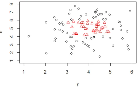
Example 3.3. The following synthetic dichotomous dataset generated by a bivariate nor-mal distribution (x∼N(5,1.5), y∼N(4,1), andρ= 0.07) with 100 instances. The dataset is called synthetic1 and used to demonstrate the implementation of SVM in nonlinear clas-sification.
Figure 3.6: Scatter plot of synthetic1
instances are used for training purpose. Recall (Section 2.2) that there is no upper bound for this value as more training instances yield better generalization. Real datasets often require normalization and feature reduction before undergoing classification. Since the SVM classifier is sensitive to distances in Hilbert space, this step is very important when dealing with attributes of different units and scales.
Normalization scales all numeric attributes in the range [0, 1] using the formula given below.
xnew = x−xmin xmax−xmin
(3.28) For the purpose of feature reduction or selecting a subset of relevant features in model building, Principal Component Analysis (PCA) has become a widely used technique. The PCA is a statistical procedure in which an orthogonal transformation is used to convert a set of observations of potentially correlated variables into a set of values of linearly un-correlated variables called principal components. Depending on the amount of variability captured by each component, the final model ends up with a fewer number of features.
3.4.1 SELECTION OFPARAMETERS
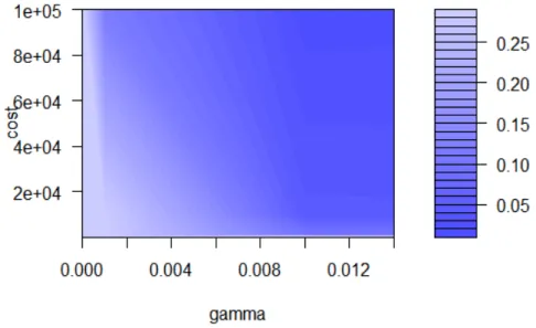
The selection of an appropriate kernel is regarded as a rule in classification experiments. We chose efficient and versatile RBF kernel to construct required SVM classifiers to standard-ize our experiments. In parameter selection, appropriate values for regularization parame-tersC andγ of the SVM classifier is found. In general, determination of these parameters are based on so called grid search. The range of value of parameters required for the search algorithm is arbitrary. In our example, the parameter values for C are 1, 10, 100, 1000, 10000, and 100000. The parameter values forγare 0.00001, 0.0001, 0.001, 0.01, 0.1, and 1. The following output file corresponds to the grid search of the regularization parameters in classifying synthetic1.
Parameter tuning of svm:
- sampling method: 10-fold cross validation
- best parameters: gamma cost
0.01 1e+05
- best performance: 0.01428571
- Detailed performance results: gamma cost error dispersion 1 1e-05 1e+00 0.28571429 0.21295885 2 1e-04 1e+00 0.28571429 0.21295885 3 1e-03 1e+00 0.28571429 0.21295885 4 1e-02 1e+00 0.28571429 0.21295885 5 1e-01 1e+00 0.28571429 0.21295885 6 1e+00 1e+00 0.04285714 0.06900656 7 1e-05 1e+01 0.28571429 0.21295885 8 1e-04 1e+01 0.28571429 0.21295885 9 1e-03 1e+01 0.28571429 0.21295885 10 1e-02 1e+01 0.28571429 0.21295885 ... ... 34 1e-02 1e+05 0.01428571 0.04517540 35 1e-01 1e+05 0.02857143 0.09035079 36 1e+00 1e+05 0.10000000 0.11761037 [email protected] 0.11761037
The R packagee1071has a built-in function for the grid search of SVM learning parameters that minimizes the training error to figure out the optimal values of the parameters. In this
case, the minimum training error is known as the best performance. Fig 3.9 illustrates the performance of the grid search in which the darker regions imply better accuracy.
Figure 3.7: Performance of SVM - grid search of learning parameters
3.4.2 TRAINING
The optimal learning parameters directly go into the training model of the SVM classifier. In general, the training procedure of the SVM requires cross validation using training data to determine the bias and support vectors. In our example, 10 fold cross validation is used. In nonlinear classification, training occurs in the high dimensional feature space and the resulting classification is mapped to the original lower dimensional space as in Fig 3.10 where the support vectors (cross sign) and nonlinear decision boundary for the whole dataset can be identified.
Figure 3.8: SVM classification plot of synthetic1
3.4.3 EVALUATION OF PERFORMANCE
Testing data is used to conclude the performance of the SVM and there are several metrics such as accuracy, precision, sensitivity, specificity, and F1 score. In more detailed analysis, average training time, number of support vectors, and Receiver Operating Characteristic (ROC) curve can be considered. The first set of metrics can be obtained through the con-fusion matrix similar to Figure 3.9. The concon-fusion matrix in itself is not a performance measure, but several useful performance metrics are based on the confusion matrix and the numbers inside it. For our case in Figure 3.9, ’Red’ refers to a positive subject and ’Blue’ refers to a negative subject.
Figure 3.9: The format of confusion matrix for synthetic1
1. Accuracy
The accuracy in classification problems is the number of correct predictions made by the model over all the predictions made. The accuracy is a strong metric if the classes in the dataset are nearly balanced.
Accuracy= T P +T N
T P +T N +F P +F N (3.29)
2. Precision
The precision a measures of the conditional probability of making a true positive decision given that the decision made is positive.
P recision= T P
T P +F P (3.30)
The sensitivity also referred as recall is a measure of the probability at which the actual positive subject is classified as positive.
Sensitivity = T P
T P +F N (3.31)
4. Specificity
The specificity is the exact opposite of the sensitivity. It is a measure of the probabil-ity at which the actual negative subject is classified as negative.
Specif icity = T N
T N +F P (3.32)
5. F1 Score
The F1 Score is designed to represent both precision and sensitivity, hence the har-monic mean of precision and sensitivity.
F1Score= 2×P recision×Sensitivity
P recision+Sensitivity (3.33) The following output file corresponds to the confusion matrix for classification of syn-thetic1.
Confusion Matrix and Statistics
Reference Prediction blue red blue 14 3
red 1 12
Accuracy : 0.8667
95% CI : 0.6928, 0.9624 No Information Rate : 0.5
P-Value [Acc > NIR] : 2.974e-05
Kappa : 0.7333 Mcnemar’s Test P-Value : 0.6171
Sensitivity : 0.9333 Specificity : 0.8000 Pos Pred Value : 0.8235 Neg Pred Value : 0.9231 Prevalence : 0.5000 Detection Rate : 0.4667 Detection Prevalence : 0.5667 Balanced Accuracy : 0.8667
’Positive’ Class : blue c@FancyVerbLinee’ Class : blue
The ROC curve is a fundamental tool for evaluation of binary classification. In a ROC curve the true positive rate (Sensitivity) is plotted against the false positive rate (1 - Specificity) for different cut-off points in classification. Each point on the ROC curve represents an ordered pair (sensitivity, specificity) corresponding to a particular decision threshold. The area under the ROC curve (AUC) is a measure of how well a classification can distinguish between two classes. The AUC measures the quality of the model’s predictions irrespective of what classification threshold is chosen.
CHAPTER 4
MULTICLASS SUPPORT VECTOR MACHINES
SVMs are originally designed for binary classification [11]. However, it can be effectively extended to multiclass classification by breaking down the multiclass classification problem into a series of binary classification problems. This technique is known as divide and conquer in computer science and still an active research area.
The three most popular multiclass SVM methods: One Vs Rest, One Vs One and Directed Acyclic Graph Support Vector Machine will be discussed in this section.
4.1 ONEVERSUS RESTSUPPORTVECTOR MACHINE
The one-vs-rest method construct k number of SVM models where k is the number of
classes.
Figure 4.1: One versus rest method: classification between 3 classes
The rth SVM is trained with all of the instances in the rth class with positive labels while the rest of instances with negative labels. Thus, givenntraining data (x1, y1), . . . ,(xn,
yn); where,xi ∈ Rn, i = 1,. . . ,nand yi ∈ {1,. . . ,k}is the class ofxi. The rth SVM solves
the following quadratic optimization problem [2]:
min1 2(w r)Twr+C n X i=1 ξir (4.1) subject to (wr)TΦ(xi) + br≥1−ξir; if yi = r, (wr)TΦ(x i) + br ≤ −1 +ξir; if yi6=r. Where,ξr
i ≥0, and i = 1, . . . ,n. Solving (4.1), leads tokdecision functions.
We can say that xi belongs to the class that has the greatest value of the decision
function [2]. A well-known drawback of the one-vs-rest method is the highly imbalanced training set for each binary classifier. Assuming equal number of training instances for all classes, the ratio of positive to negative instances for each binary classifier is 1/(k−
1). Hence, the original problem loses the symmetry of classification, affecting the results; especially, sparse classes may suffer seriously [12, 16, 18].
4.2 ONE VSONESUPPORTVECTORMACHINE
The one-vs-one method aims to get rid of the imbalance problem of the one-vs-rest method by training binary classifiers only with the data belong to two original classes designated by each classifier. The one-vs-one method constructsk(k−1)/2given thatkis the number of classes [17, 19, 20].
Figure 4.2: One against one method: classification between 3 classes
i-vs-j classifier solves the following quadratic optimization problem.
min1 2(w ij )Twij +C n X i=1 ξiij (4.2) subject to (wij)TΦ(x t) + bij ≥1−ξiij ; if yt= i, (wij)TΦ(x t) + bij ≤ −1 +ξiij ; if yt= j. Where,ξtij ≥0, and t = 1, . . . ,n
After all classifiers are constructed, we can use the following voting strategy: If the sign of i-vs-j classifier says that xt is in the ith class, then the vote for the ith class is
increased by 1. Otherwise, the vote for the jthclass is increased by 1. Finally, we conclude thatxtis in the class with the highest vote. This type of voting approach is called the ”Max
Wins” strategy. In the case that votes for two classes tie, we simply select the one with the smaller index [2].
4.3 DIRECTEDACYCLIC GRAPH SUPPORTVECTOR MACHINE
The Directed Acyclic Graph Support Vector Machine is constructed by introducing one-vs-one classifiers into the nodes of a decision Directed Acyclic Graph (DAG).
Figure 4.3: Input space of a 4 class problem
Definition 4.1. A decision DAG on k number of classes over a set of Boolean functions
F = {f :X 7→ {0,1}} for a given space X is a function that uses a rooted binary DAG withkleaves labeled with the classes where each of thek(k-1)/2internal nodes is labeled with an element of F. The nodes are setup in triangular shape with a root node at the top two nodes in the 2nd layer and so on. The final layer has k leaves. The ith node in layer j < k is joined to theithand(i+ 1)stnode in the(j + 1)st layer [6].
For an input x∈X , of a decision DAG, starting at the root node, each node is exited via the left edge, if the binary function is 0 or the right edge, if the binary function is 1, until x meets a leaf. The corresponding output of the decision DAG is the value associated with the leaf. This particular path taken through the decision DAG is called evaluation path [6]. In the case of the DAGSVM, we use binary values -1 and +1. The DAGSVM has the following properties.
1. Nodes of the DAGSVM are maximum margin classifiers over a kernel induced fea-ture space. Hence maximizing the margin of every node of the decision DAG results in a smaller generalization error bound.
2. It is safe to ignore the losing class at each binary decision, since all of the instances of the losing class are far away from the decision boundary as shown in Figure 4.3. 3. For the DAGSVM, the order of choosing the binary classifiers is arbitrary.
Lim-ited experimentations show that changing this order does not significantly affect the accuracy of the algorithm.
4. The DAGSVM is superior to other two multiclass support vector machine algorithms in both training and evaluation time.
CHAPTER 5
FAST MULTICLASS CLASSIFICATION 5.1 CURSE OFDIMENSIONALITY
The curse of dimensionality refers to various issues related to analyzing and organizing data in very high-dimensional spaces. The expression was coined by Richard E. Bellman in a highly acclaimed article considering problems in dynamic optimization [13, 14]. In general, as dimensionality increases, the volume of the space increases rapidly and the data becomes sparser. The sparsity of data is problematic for any method that requires statistical significance. In order to obtain a statistically sound and reliable result, the amount of data needed often grows exponentially with the dimensionality, which prevents common data mining techniques from being efficient; often leading to over-fitting.
Recall that the SRM provides tools to investigate the generalization ability of the SVM under the curse of dimensionality. Since the VC dimension of the SVM classifier grows with the dimensionality of the data points, from (2.3) we can assume that the VC confidence also increases with the dimensionality of the data points. Consider the following example.
Example 5.1. Figure 5.1 shows how the VC confidence varies with VC dimension/number of training data (h/n). For of 95% confidence level (η =0.05) and a training sample of size 10,000, the VC confidence is an increasing function of h/n.
Hence, it is clear that when the dimensionality increases relative to the number of training instances, the upper bound of the true risk increases. As a result, the SVM suffers from over-fitting.
Figure 5.1: VC confidence against VC dimension/number of training data
5.2 DIVIDE ANDCONQUERSUPPORTVECTOR MACHINE (DCSVM)
In this section we present a SVM-based multiclass classification method called the Divide and Conquer Support Vector Machine (DCSVM) that exploits the curse of dimensionality to efficiently perform classification of high dimensional data.
The DCSVM algorithm idea is based on the following simple observation, best de-scribed using the example in Figure 5.2. The figure shows 6 classes (1 – red, 2 – blue, 3 – green, 4 – black, 5 – orange, and 6 – maroon) of two-dimensional points and a lin-ear SVM separation of classes 1 and 2 (the line that separates the points in these classes). It happens that the SVM model for classifying classes 1 and 2 completely separates the points in classes 4 (which takes class 2 side) and 6 (which takes class 1 side). Moreover, the classifier does a relatively good job classifying most points of the class 5 as class 2 (with relatively few points classified as 1) and a poor job on classifying the points of class 3 (as the points in this class are classified about half as 1’s and the other half as 2’s). With
DCSVM we use the SVM classifier for classes 1 and 2 for a candidate of an unknown class: if the classifier predicts 1, then we next decide between classes 1, 6, 3, and 5; if the classifier predicts class 2, then we next decide between classes 2, 4, 3, and 5. Notice that in either case one or more classes are eliminated and we are left to predict a fewer classes. That is, a multi-class classification problem of a smaller size (less classes). The algorithm then proceeds recursively on the smaller problem. Given that the number of classes isk, in the best case scenario, half of the classes will be eliminated at each step and the algorithm will finish inlog2ksteps. Notice that, in the above scenario, classes 2 and 4 are completely separated from classes 1 and 6, whereas classes 3 and 5 are not clearly on one side or the other of the separation line. For this reason, classes 3 and 5 are part of the next decision step, regardless of the prediction of the first classifier.
However, there is a significant difference between classes 3 and 5. While class 3 is almost divided in half by the separation line, class 5 can be predicted as ”2” with a very small error. In DCSVM we use a threshold value to indicate the maximum classification error accepted in order to consider a class on one side or the other of a separation line. For instance, let us consider that only 2% of the points of class 5 are on the same side as class 1. With the threshold value set to 0.02, DCSVM will separate classes 1, 3, and 6 (when 1 is predicted) from classes 2, 3, 4, and 5 (when 2 is predicted). A higher threshold value will produce a better separation of classes (less overlapping) and less classes to process in the subsequent steps. This comes at the price of possibly sacrificing the accuracy of the final prediction. Clearly, the method presented in the example above is in general suitable for multiclass classification using a binary classifier. Our choice of using SVM is based on the SVM algorithm’s remarkable power in producing accurate binary classification.
Figure 5.2: Seperation of classess 1 and 2 by a linear SVM classifier
5.2.1 ARCHITECTURE OF DCSVM
Let us first introduce some notations, next we will proceed to the formal description of the algorithm. Given a data set of k classes (labels) D where each data itemx ∈ Dhas been assigned a label l ∈ {1, . . . , k}, we want to construct a decision function dcsvm :
D → {1, . . . , k}so thatdcsvm(x) = l, wherel is the corresponding label of x ∈ D. By considering a split D= R∪T of the data setDinto two disjoint setsR(the training set) and T (the test set), we use the data inR to construct our decision functiondcsvm()and then the data inT to measure its accuracy. Furthermore, we considerR =R1∪R2∪· · ·∪Rk
as an union of disjoint setsRl, where eachx ∈Rlhas labell,l = 1, . . . , k. (Similarly, we
considerT =T1∪T2∪ · · · ∪Tkas an union of disjoint setsTl, where eachx∈Tlhas label l,l = 1, . . . , k.)
Let svmi,j : D → {i, j}, be a SVM binary classifier created using the training set Ri∪Rj,i < jandi= 1, . . . , k−1, j = 2, . . . , k. There arek(k−1)/2such one-versus-one
binary classifiers. It is important to mention that the svm()decision function considered here is not the ideal one, but the practical one, likely affected by misclassification errors; that is, for somex∈Ri∪Ti, we may have thatsvmi,j(x) =j.
Our goal is to create thedcsvm()decision function that uses a minimal number of bi-nary decisions fork-classes classification, while not sacrificing the classification accuracy. Next, we define a few measures we use in the process of identifying the shortest path to a multi-class classification decision.
Definition 5.1. (Class Predictions Likelihoods) The class predictions likelihoods of a SVM binary classifiersvmi,j(·)for a label l ∈ {1, . . . , k}, denoted respectively asCi,j(l, i) and
Ci,j(l, j), are: Ci,j(l, i) = |{x∈Rl |svmi,j(x) =i}| |Rl| Ci,j(l, j) = |{x∈Rl |svmi,j(x) =j}| |Rl| = 1−Ci,j(l, i) (5.1)
Each class prediction likelihood represents the expected outcome likelihood for ior
j when a binary classifier svmi,j(·)is used for prediction on all data items in Rl. These
likelihoods are computed for each binary classifier and each class in the training data set. All pairs of likelihood predictions, for every binary classifiersvmi,j(·)and classes are
stored in a table, called All-Prediction table.
Definition 5.2. (All-Prediction Table) We arrange all classes predictions likelihoods in rows (corresponding to each binary classifiersvmi,j) and columns (corresponding to each
class1, . . . , k) to form a table T where each entry is given by a pair of predictions likeli-hoods as follows:
T[svmi,j, l] = (Ci,j(l, i),Ci,j(l, j)) (5.2)
Fig 5.2 shows the All-Predictions table computed for the glass dataset [15]. The dataset contains 6 classes, labeled as 1, 2, 3, 5, 6, and 7. Each row corresponds to a binary classifier svm1,2,· · · , svm6,7and columns correspond to each class label. Each ta-ble cell contains a pair of likelihood predictions (as percentages) for the row classifier and class column. For instance, C1,2(1,1) = 100%, C1,2(1,2) = 0% andC1,6(2,1) = 91.8%, C1,6(2,6) = 8.2%.
Figure 5.3: Prediction plan of glass for threshold = 0.05
Next, we define two measures for the quality of the classification of each svmi,j(·).
The Impurity Index measures how good the binary classifier is for classifying all classes as
iorj for a given likelihood thresholdθ. In a nutshell, a classl is classified as ”definitely”
i by svmi,j(·) if Ci,j(l, i) ≥ 1−θ; as ”definitely” j if Ci,j(l, j) ≥ 1−θ; otherwise, it
decisions a binary classifier produces. The lower the index, the better the separation. The Balance Index measures how ”balanced” a separation is in terms of the number of classes predicted asiandj. The larger the index, the better the separation.
Definition 5.3. (SVM Impurity and Balance Indexes) For an likelihood threshold θ of a SVM classifiersvmi,j(·), we define:
the Impurity Index, denoted asPi,j(θ), as:
Pi,j(θ) = k X l=1 (χθ(Ci,j(l, i)) +χθ(Ci,j(l, j))) ! −k (5.3)
the Balance Index, denoted asBi,j(θ), as:
Bi,j(θ) = min k− k X l=1 χθ(Ci,j(l, j)), k− k X l=1 χθ(Ci,j(l, i)) ! (5.4) whereχθis the step function:
χθ(x) = 1 ifx > θ 0 ifx≤θ
For instance, the Impurity Index for rowsvm1,6and thresholdθ = 0.05in Fig 5.2 is: P1,6(0.05) = ((1 + 0) + (1 + 1) + (1 + 0) + (1 + 1) + (0 + 1) + (1 + 1))−6 = 3
and indicates that 3 of the classes (namely 2, 5, and 7) are undecided when the required precision is at leastθ = 5%.
For likelihood threshold θ = 0.05, the Balance Index for row svm1,2 in Fig 5.2 is B1,2 = 1and for rowsvm5,6 isB5,6 = 2.
The SVM Score, defined below, is a measure of the sensitivity of the binary classifier
svmi,j(·)for classifying classesiandj. The higher the Score the better the classifier. Definition 5.4. (SVM Score) The Score of a SVM classifier svmi,j(·) is its sensitivity,
denoted bySi,j, is
Si,j =
Ci,j(i, i) +Ci,j(j, j)
For instance, the table in Fig 5.2 shows that S1,2 = C1,2(1,1) +C1,2(2,2) 2 = 100% + 100% 2 = 100%. Algorithm 1DCSVM training
1: procedureTRAINDCSVM(R1, . . . , Rk, θ) .Creates DCSVM classifier 2: Input:R =R1, . . . , Rk: data set,θ: likelihood threshold
3: Output:dcsvm()
4: svmi,j ←train SVM withRi∪Rj,i= 1, . . . , k−1,j = 2, . . . , k,i < j 5: T[svmi,j, l] = (Ci,j(l, i),Ci,j(l, j)), for allsvmi,j,l = 1, . . . , k
6: //Recursively construct a binary decision tree
7: //with each node associated with asvmi,jbinary classifier 8: dcsvm←empty binary tree
9: dcsvm.root←new tree node
10: DCSVM-SUBTREE(dcsvm.root,T, θ)
11: returndcsvm .Returns the decision tree
12: end procedure
Algorithm 1 and 2 describe DCSVM training and proceeds as follows. In the main procedure, TRAINDCSVM, the SVM binary classifiers for all class pairs are trained (line
4) and the predictions likelihoods are stored in the predictions table (line 5). The deci-sion function dcsvm is created as an empty tree (line 8) and then recursively populated in DCSVM-SUBTREEprocedure (line 10). The recursion procedure creates a left and/or a right node at each step (lines 12 and 19, respectively) or may stop with creating a left and/or a right label (lines 9 and 16, respectively). Each new node is associated to the binarysvmi,j
that is the decider at that node (line 5), or with a class label if an end node (lines 9 and 16).
An important part of the DCSVM-SUBTREE procedure is choosing the ”optimal”
Algorithm 2DCSVM training (continued)
1: procedureDCSVM-SUBTREE(pnode,T, θ) .Creates subtree routed atpnode
2: Input: pnode: current parent node,T: current predictions table,θ: likelihood thresh-old
3: Output: recursively constructs sub-tree rooted atpnode
4: svmi,j ←optimalsvminT, for givenθ 5: pnode[svm]←svmi,j
6: listi←classes labeled asior undecided bysvmi,j 7: listj ←classes labeled asjor undecided bysvmi,j
8: iflength(listi) = 1then .reached a leaf
9: pnode.lef tnode←tree-node(label inlisti)
10: else
11: T.lef t ← T minus svmm,n, m ∈ listj or n ∈ listj rows, and columns of
classes not inlisti
12: pnode.lef t←new tree node
13: DCSVM-SUBTREE(pnode.lef t,T.lef t, θ)
14: end if
15: iflength(listj) = 1then .reached a leaf
16: pnode.rightnode←tree-node(label inlistj)
17: else
18: T.right ← T minussvmm,n, m ∈ listi or n ∈ listi rows, and columns of
classes not inlistj
19: pnode.right←new tree node
20: DCSVM-SUBTREE(pnode.right,T.right, θ)
21: end if 22: end procedure
SVM Impurity Index, Balance Index, and Score from Definitions 9 and 10, respectively. The order these measures are used may influence the decision tree shape and precision. If Score is used then the Impurity and Balance Indexes are used to break a tie, the resulting tree favors accuracy over the speed of decisions (may yield bushier trees). If Impurity and Balance Indexes are used first, then Score, if a tie, the resulting tree may be more balanced. The decision speed is favored while possibly sacrificing accuracy.
Adcsvm decision tree for theglassdata set is shown in. Clearly, the algorithm may produce highly unbalanced dcsvm decision trees (when some classes are decided faster than others) or very balanced decision trees (when most of class labels are leaves situated at about same depth). Regardless of outcome, the following result is almost immediate.
Proposition 5.2. Thedcsvmdecision tree constructed in Algorithm 2 has depth at mostk.
Proof. The lists of classes labeled i and j (lines 6, 7 in DCSVM-SUBTREE procedure) contain at least one label each: iandj, respectively. Once a class column is removed from T at some tree noden, it will not appear again in a node or leaf in the subtree rooted at that node n. Hence with each recursion the number of classes decreases by at least one (lines 11, 18) fromk to 1, ending the recursion with a left or a right label node in lines 9 or 16, respectively.
Notice that a scenario where each dcsvm decision tree label has depthk is possible in practice: when no svmi,j binary classifier is a good separator for classes other than i and j (and therefore at each node only classes i and j are separated, while the other are undecided and will appear in both left and right branches). We call this the worst case scenario, for obvious reasons. The opposite case scenario is also possible in practice: eachsvmi,j separates all classes into two disjoint lists of about same lengths. Thedcsvm
decision tree is also very balanced in this case, but a lot smaller.
Proposition 5.3. Thedcsvm decision tree constructed in Algorithm 2 when each svmi,j produced balanced, disjoint separation between all classes has depth at mostdlog2ke.
Proof. Clearly this is a case scenario where at each recursion step a node is created such that half of the classes are assigned to the left subtree and the other half to the right subtree. This produces a balanced binary tree withkleaves, hence of depth at mostdlog2ke.
Algorithm 3DCSVM classifier
1: procedureDCSVMCLASSIFY(dcsvm,x) .Produces DCSVM classification
2: Input:dcsvm: decision tree;x: data item
3: Output: Label of data itemx 4: node←dcsvm.root
5: whilenodenot a leafdo .Visits the decision tree nodes towards a leaf
6: svmi,j ←node[svm] .Retrieves thesvmassociated to current node
7: label←svmi,j(x) 8: iflabel=ithen 9: node←node.lef t 10: else 11: node←node.right 12: end if 13: end while
14: returnlabel ofnode .Returns the leaf label 15: end procedure
The DCSVM classifier Algorithm 3 relies on the dcsvm decision tree produced by Algorithm 1 to take any data itemxand predict its label. The algorithm starts at the decision tree root node (line 4) then each node’s associatedsvmpredicts the path to follow (lines 6– 12) until a leaf node is reached. The label of the leaf node is the DCSVM’s prediction (line 14) for the input data item x. An example of prediction path in a dcsvmtree is illustrated in Fig 5.4 (b).
Theorem 5.4. The Algorithm 3 performs multi-class classification of any data item xin at most k binary decisions steps (in the worst case scenario) and at mostdlog2ke binary decision steps (in the best case scenario).
We illustrate next how the dcsvm decision tree is created and how a prediction is computed using a working example.
5.2.2 A WORKING EXAMPLE
We use theglassdataset [15] to illustrate DCSVM at work. This data set contains 6 classes, labeled 1, 2, 3, 5, 6, and 7 (notice there is no label 4). Consequently,6∗(6−1)/2 = 15
binary svm classifiers are created and then the All-Predictions table T is computed as shown in Figure 5.3. Let us choose the likelihood thresholdθ = 0, for simplicity. That is, a classl is classified by ansvmi,j as onlyiifsvmi,j predicts that all data items inRlhave
classi;lis classified as onlyj ifsvmi,j predicts that all data items inRlhave classj; else, l is undecided and will appear on both sides of the decision tree node associated tosvmi,j.
We follow next the DCSVM-SUBTREE procedure in Algorithm 2 and construct the
dcsvm decision tree. Notice thatSi,j = 100% for allsvmi,j, so Score does not matter for
choosing the optimalsvmi,j in line 4. The choice will be solely based on the Impurity and
Balance indexes. Table 5.1 shows all values for these measures obtained form the initial
All-Predictionstable.
It is clear that rows 1, 13, and 14 as candidates with minimum Impurity Indexes. Then there is a tie between rows 13 and 14 as the winners among these. Row 13 comes first and hencesvm5,6 is selected as the root node. Figure 5.4 (a) shows the full decision tree, with svm5,6as the root node. Subsequently,svm5,6labels classes 1, 2, 3, and 5 as ”5” (left), and classes 6 and 7 as ”6” (right). The algorithm continues recursively with classes{1,2,3,5} to the left, and classes{6,7}to the right. The right branch will be completed immediately with one more tree node (for svm6,7) and two corresponding leaf nodes (for labels 6 and
Table 5.1: svmoptimality measures forglassdataset and the initialAll-Predictionstable
svmi,j Pi,j(0) Bi,j(0) Si,j
1. svm1,2 0 1 100% 2. svm1,3 4 1 100% 3. svm1,5 3 1 100% 4. svm1,6 3 1 100% 5. svm1,7 3 1 100% 6. svm2,3 3 1 100% 7. svm2,5 1 2 100% 8. svm2,6 3 1 100% 9. svm2,7 2 1 100% 10. svm3,5 2 1 100% 11. svm3,6 1 1 100% 12. svm3,7 3 1 100% 13. svm5,6 0 2 100% 14. svm5,7 0 2 100% 15. svm6,7 4 1 100%
(a) (b)
Figure 5.4: DCSVM decision tree with (a) the decision process for glass dataset (b) the classification of an unseen instance
7).
For the left branch the algorithm will proceed with a reduced All-Predictions table: rows 4, 5, 8, 9, 11, 12, 13, 14, and 15 and columns for classes 6 and 7 are removed. The optimality measures will be subsequently computed for all svm and classes still in competition (1, 2, 3, and 5) in the left branch. The corresponding measures are given in Table 5.2 (for an easier identification, the indexes in the first column are kept the same as the original indexes in theAll-Predictionstable in Figure 5.3).
There is a tie between svm1,2 andsvm2,5, and svm1,2 is being used first. A node is consequently created, with a leaf as a left child. The rest of the tree is subsequently created in the same manner.
5.3 EXPERIMENTS
We implemented DCSVM in R v3.4.3 using e1071 library [21], running on Windows 10, 64-bit Intel Core i7 CPU @3.40GHz, 16GB RAM. For testing we used 14 data sets from
Table 5.2: Optimality measures in the second step of creating the decision tree in Figure 5.3 (b)
svmi,j Pi,j(0) Bi,j(0) Si,j
1. svm1,2 0 1 100% 2. svm1,3 2 1 100% 3. svm1,5 1 1 100% 6. svm2,3 1 1 100% 7. svm2,5 0 1 100% 10. svm3,5 2 1 100%
UCI repository [15] (listed in Table 5.3). For each experiment, we used cross-validation with 80% data for training and 20% for testing, for each data set. We ran 10 trials and averaged the results. We ran three sets of experiments: (i) multi-class prediction accuracy, (ii) prediction performance in terms of speed (time and number of binary decisions) and resources (number of support vectors), and (iii) DCSVM performance comparisons for different data sets and accuracy threshold parameter values. For the first set of experiments we compared three multi-class predictors: build-in multi-class SVM (LibSVM from the e1071 library), R implementation of One-Vs-One, and R implementation of DCSVM. For a fair comparison, in the second set of experiments we compared R implementations of One-Vs-One and DCSVM. The built-in multi-class SVM would benefit of the inherent speed of native code it relies on. Finally, the third set of experiments focused on the DCSVM’s R implementation performance and fine tuning.
5.4 RESULTS
This section summarizes the results of the experiments described in the chapter 5.2.2. To calculate the accuracy of each experiment, the method in (3.29) is used. In graphs, two
different scales are used to illustrate the maximum disparity of information whenever re-quired.
5.4.1 COMPARISON OFACCURACY
The main goal of DCSVM is to improve multi-class prediction performance while not sacrificing the prediction accuracy. The first experimental results compare multi-class pre-diction accuracy of: (i) built-in SVM multi-class prepre-diction (in the e1071 package), (ii) one-versus-one implementation in R, and (iii) DCSVM implementation in R. The results are displayed in Figure 5.5 and show no significant differences between the three methods.
Figure 5.5: Average prediction accuracy (%)
5.4.2 PREDICTION PERFORMANCECOMPARISON
For this purpose we compared the R implementations of One-Vs-One method and DCSVM. We analyzed prediction performance on three aspects: the average number of support
vec-tors, the average number of binary decisions, and average prediction time. The correspond-ing performance results are presented in Figure 5.6, Figure 5.7 and Figure 5.8 respectively. The number of support vectors used was computed by summing up all support vectors from every binary decider, over all steps of binary decisions until the multi-class prediction was achieved. The number of such support vectors is clearly proportional not only to the num-ber of decision steps (which are illustrated separately), but also to the configuration of data separated by each binary classifier. It is clear that DCSVM significantly outperforms One-Vs-One, clearly being much less computationally intensive (number of support vectors for prediction) and faster (number of binary decisions and prediction times).
Figure 5.6: Average number of support vectors
5.4.3 DCSVM PERFORMANCEFINETUNING
In this set of experiments we analyze in close detail DCSVM’s performance in terms of the likelihood threshold parameter. Figure 5.9 shows the trade-off between accuracy (left) and the average prediction steps (right) with various threshold values. Clearly, the likelihood threshold parameter permits a trade-off between accuracy and speed. However, this is largely data dependent. The more separable the data is, the less influence the threshold
Figure 5.7: Average number of steps
Figure 5.8: Average prediction time (sec)
has on speed. For less separable data (such as the letter data set), fine adjustment of the threshold permits trade-off between prediction accuracy and prediction speed. This is not the case for the vowel dataset, which is highly separable: changes in the threshold influence neither the accuracy of prediction nor the average number of prediction steps.
Table 5.4 shows side-by-side accuracies of multi-class classification using (i) built-in (BI), (ii) one-against-one (OvsO), and (iii) DCSVM (for a few threshold valuesθ). DCSVM performs very well in terms of accuracy (compared to the other methods) for all data sets,
Figure 5.9: Accuracy and the average number of prediction steps for different likelihood thresholds
for threshold values θ ∈ {2%,1%,0.1%,0.01%} (the larger the threshold, the better the accuracy, in general). A larger threshold θ may increase the prediction speed (Table 5.5) and reduce the computation effort (Table 5.6). Interesting to notice: Table 5.5 shows that in all cases displayed in the table the number of decision steps is less thank−1, wherekis the number of classes in the respective data set. DCSVM outperforms (even for very small threshold) one-against-one and its improvement DAGSVM [6], which reaches multi-class prediction afterk−1steps.
The All-Predictions table in Figure 5.3 collects all information used by DCSVM to construct its multi-class prediction strategy (the dcsvm decision tree in Algorithm 1 and 2). The same information can be used to predict how much separation can be achieved for different threshold values. For instance, for the glassdataset All-Predictions table in Figure 5.3 and for a threshold value θ = 2% there are 58 entries in the table where the percentage of predicting one class or the other is at least100−θ = 98%(out of a total of
15×6 = 80 entries in the table). The percentage58/80 = 72.5% is a good indicator of purity for DCSVM with thresholdθ= 2%: the higher the percentage, the more separation is produced at each step and hence a shallow decision tree.
and four data sets (letter, vowel, usps, andsensorless). Intuitively, as threshold increases so does the separation percentage. Theletteranduspsdata sets display an almost linear in-crease of separation with threshold.sensorlessdisplays a sharp increase for small threshold values, then it tends to flatten, that is, not much gain for significant increase in threshold (and hence possibly less accuracy). Lastly, voweldisplays a step-like behavior: not much gain in separation until threshold value reaches approximatelyθ = 2.3%, a steep increase untilθ approaches3%, then nothing much happens again. One can use these indicators to decide the trade-off between speed and accuracy of predictions.
Table 5.3: Prediction accuracies for different split thresholds
DCSVM
No Dataset LibSVM O-V-O θ = 2 θ = 1 θ = 0.1 θ = 0.01
1 artificial1 98.85 98.76 98.70 98.70 98.76 98.76 2 iris 96.97 96.97 96.97 96.97 96.97 96.97 3 segmentation 27.71 27.71 29.44 29.44 29.44 29.44 4 heart 58.82 58.82 59.12 59.12 59.12 59.12 5 wine 96.97 96.97 96.97 96.97 96.97 96.97 6 wine-quality 62.33 62.33 62.39 62.39 62.39 62.39 7 glass 87.55 91.70 91.29 91.29 91.29 91.29 8 covertype 49.95 49.95 49.95 49.95 49.95 49.95 9 svmguide4 57.88 71.21 72.73 72.73 72.73 72.73 10 vowel 94.34 97.26 97.26 97.26 97.26 97.26 11 usps 94.17 93.94 93.89 94.08 94.17 94.17 12 letter 95.25 96.43 95.52 96.00 96.41 96.41 13 poker 55.94 55.96 55.56 55.83 55.96 55.96 14 sensorless 97.46 98.87 98.32 98.60 98.86 98.87
Table 5.4: DCSVM: average number of steps per decision for different split thresholds No Dataset θ = 2 θ = 1 θ = 0.1 θ= 0.01 1 artificial1 3.76 3.75 3.67 3.67 2 iris 1.71 1.71 1.71 1.71 3 segmentation 5.63 5.63 5.63 5.63 4 heart 4.00 4.00 4.00 4.00 5 wine 1.69 1.69 1.69 1.69 6 wine-quality 4.85 4.86 4.87 4.87 7 glass 4.09 4.12 4.12 4.12 8 covertype 5.93 5.93 5.93 5.93 9 svmguide4 4.63 4.88 4.88 4.88 10 vowel 5.41 5.41 5.41 5.41 11 usps 7.16 7.29 7.80 7.80 12 letter 17.63 19.56 22.29 22.29 13 poker 8.36 8.40 8.43 8.43 14 sensorless 5.44 5.49 6.28 6.93