*Corresponding author:Vijaya Kumar R ISSN: 0976-3031
Research Article
CONSTRUCTION OF MIXED SAMPLING PLAN WITH SINGLE SAMPLING PLAN AS
ATTRIBUTE PLAN INDEXED THROUGH MAPD AND AQL USING IRPD
Vijaya Kumar R
1and Sampath Kumar R
21
Department of Statistics, St. Joseph’s College, Tiruchirappalli – 02
2
Department of Statistics, Government Arts College, Coimbatore
DOI: http://dx.doi.org/10.24327/ijrsr.2019.1008.3823
ARTICLE INFO ABSTRACT
This paper presents the procedure for the construction and selection of mixed sampling plan (MSP) using Intervened Random effect Poisson Distribution (IRPD) as a baseline distribution. Having the Single sampling plan as attribute plan, the plans are constructed through acceptable quality level (AQL) and maximum allowable percent defective (MAPD). Tables are constructed for easy selection of the plan.
INTRODUCTION
Mixed sampling plans consist of two stages of rather different nature. During the first stage the given lot is considered as a sample from the respective production process and a criterion by variables is used to check process quality. If process quality is judged to be sufficiently good, the lot is accepted. Otherwise the second stage of the sampling plan is entered and lot quality is checked directly by means of an attribute sampling plan. There are two types of mixed sampling plans called independent and dependent plans. If the first stage sample results are not utilized in the second stage, then the plan is said to be independent otherwise dependent. The principal advantage of mixed sampling plan over pure attribute sampling plan is a reduction in sample size for a similar amount of protection.
Schilling (1967) proposed a method for determining the operating characteristics of mixed variables – attributes sampling plans, single sided specification and standard deviation known using the normal approximation. The mixed sampling plans have been designed under two cases of significant interest. In the first case, the sample size n1 is fixed
and a point on the OC curve is given. In the second case, plans are designed when two points on the OC curve are given. Devaarul (2003) has studied the mixed sampling plans and reliability based sampling plans.
Sampath Kumar (2007) has constructed mixed variables – attributes sampling plans indexed through various parameters. Sampath Kumar et.al (2012)have made contributions to mixed sampling plans for independent case
In the product control, the defective units are either rebuilt or replaced by new units during the sampling period. Quality engineers are always interested in improving the quality level of the product to enhance the satisfaction of the customers and hence, they keep making changes in the production process. These actions trigger a change in the expected incidence of defective items in the remaining observational period. Any action for reducing the number of defectives during the sampling period is called an intervention and such intervention parameter ranges from 0 to 1.
In Intervened Random effect Poisson Distribution (IRPD), Poisson parameter is modified in two ways: one method is multiplying an intervention parameter ρ (a constant) and
Available Online at http://www.recentscientific.com
International Journal of
Recent Scientific
Research
International Journal of Recent Scientific Research
Vol. 10, Issue, 08(B), pp. 34113-34117, August, 2019
Copyright © Vijaya Kumar R and Sampath Kumar R, 2019, this is an open-access article distributed under the terms of the Creative Commons Attribution License, which permits unrestricted use, distribution and reproduction in any medium, provided the original work is properly cited.
DOI: 10.24327/IJRSR
CODEN: IJRSFP (USA)
Article History: Received 4th May, 2019
Received in revised form 25th June, 2019 Accepted 18th July, 2019
Published online 28th August, 2019
Key Words:
secondly, multiplying an unobserved random effect which follows Gamma probability distribution. The IRPD can be very useful to the quality and reliability engineers, who always make changes in the production system in the observational period of quality checking to ensure reliability of the system, because, the failure rate of the components may vary in different time intervals. The other areas of application of IRPD are queuing, demographic studies and process control and so on.
Shanmugam (1985) has used Intervened Poisson Distribution (IPD) in the place of Zero Truncated Poisson Distribution (ZTPD) for the study on cholera cases. Radhakrishnan and Sekkizhar (2007a, b, and c) introduced Intervened Random effect Poisson Distribution in the place of Poisson distribution for the construction of attribute sampling plans.
In this paper, using the operating procedure of mixed sampling plan (independent case) with single sampling plan as attribute plan, tables are constructed using IRPD as a baseline distribution. The tables are constructed for mixed sampling plan (MSP) indexed through i) AQL and ii) MAPD. The plan indexed through MAPD is compared with the plan indexed through AQL.
Conditions for Applications of IRPD – Mixed Sampling Plan
Production process is modified during the sampling inspection by an intervention.
Lots are submitted substantially in the order of their production.
Inspection is by variable in the first stage and attribute in the second stage with quality defined as a fraction defective.
Lot quality variation exists.
Glossary of symbols
The symbols used in this paper are as follows:
p
: submitted quality of lot or process( )
a
P p
: probability of acceptance for given quality ’p
’1
p
: submitted quality such that Pa (p1) = 0.95 (also called AQL)*
p
: maximum allowable percent defective (MAPD) n : sample size for each lotn1 : sample size for variable sampling plan
n2 : sample size for attribute sampling plan
j
: probability of acceptance for the lot quality ‘p
j’j
: probability of acceptance assigned to first stage for percent defective ‘p
j’j
: probability of acceptance assigned to second stage for percent defective ‘p
j’z (j) : ‘z’ value for the jth ordered observation
k : variable factor such that a lot is accepted if
X
U
k
Operating Procedure of Mixed Sampling Plan Having Single Sampling Plan As Attribute Plan
The general procedure given by Schilling (1967) for the independent mixed sampling plan with upper specification limit (U) and standard deviation (σ).
Select a random sample of size n1 from the lot assumed to be
large
1. If the sample average
X
≤ A = U - k
, accept the lot.2. If the sample average
X
> A = U - k
, take a second sample of size n2.3. Inspect and find the number of defectives‘d’ in the second sample.
If the number of defectives d ≤ c, accept the lot. If the number of defectives d > c, reject the lot.
Construction of Mixed Sampling Plans with Single Sampling Plan As Attribute Plan Using IRPD
Schilling (1967) has given the OC function of mixed sampling plan as
( )
L p
=Pn1(X
A)+Pn1(X
>A)
2
0;
c
j
p j n
(1)The above expression is given as
j
=
j
+(1-
j
)
j
(2) The operation of mixed sampling plans can be properly assessed by the OC curve for given values of the fraction defective. The development of mixed sampling plans and the subsequent discussions are limited only to the upper specification limit ‘U’. By symmetry, a parallel discussion can be made for lower specification limits.The procedure for the construction of mixed variables – attributes sampling plans is provided by Schilling (1967) for a given n1, n2, i, k and a point ‘
p
j’ on the OC curve is givenbelow.
Assume that the mixed sampling plans are independent Split the probability of acceptance (
) determining theprobability of acceptance that will be assigned to the first stage. Let it be
j
Decide the sample size n1 (for variable sampling plan) to
be used
Calculate the acceptance limit for the variable sampling plan as
1
[ (
j) { (
j) /
}]
U
k
U
z p
z
n
,where U is the upper specification limit and z (t) is the standard normal variate corresponding to ‘t’ such that t =
( )
1
2
z t
e
u2/ 2du
Determine the sample average
X
. If a sample averageX
>
U
k
, take a second stage sample size ‘n 2’ Split the probability of acceptance
j as
j
and
j
, such that
j =
j
+ (1-
j
)
j
. Fix the value of
j
. Now determine
j
, the probability of acceptance assigned to the attributes plan associated with the second stage sample as
j
=(
j -
j
)/(1-
j
) Determine the appropriate second stage sample size ‘n2’
from
P p
a( )
=
j
forp
=p
jUsing the above procedure, tables can be constructed to facilitate easy selection of mixed sampling plan with single sampling plan as attribute plan using IRPD as a baseline distribution indexed through MAPD and AQL.
Sekkizhar (2007) suggested the probability mass function of IRPD for the Single Sampling Plan (SSP) as
( )
a
P p
=
0 0
1 !
1 ! ! 1 !
1 l x c x x l l e
l x l
When α=1,
P p
a( )
=
0 01
1
!
1
l x c x x le
x
l
, where1
np
(3)Using the above procedure, tables can be constructed to facilitate easy selection of MSP using IRPD as a baseline distribution. The tables furnished in this paper are for the case when α=1.
Construction of MSP with SSP as attribute plan indexed
Through MAPD using IRPD
MAPD, introduced by Mayer (1967) and studied by Soundararajan (1975) is the Quality level corresponding to the inflection point of the OC curve. The degree of sharpness of inspection about this quality level ‘
p
*’ is measured by ‘p
t’, the point at which the tangent to the OC curve at the inflection point cuts the proportion defective axis. For designing, Soundararajan (1975) proposed a selection procedure for single sampling plan indexed with MAPD and R=ptp*
.
Using the probability mass function of the IRPD, given in expression (3), the inflection point (
p
*) is obtained by using2 2
( ) 0
a
d P p
dp = and
3 3
( )
a
d P p
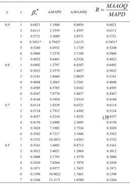
dp ≠0. The n2MAPD values are
calculated for different values of cand ρ for
*
0.30 usingC program and presented in Table 1.
The MAAOQ (Maximum Allowable Average Outgoing Quality) of a sampling plan is defined as the Average Outgoing Quality (AOQ) at the MAPD.
By definition AOQ =
p
P p
a( )
and MAAOQ =p
*P p
a(
*)
The values of MAPD and MAAOQ are calculated for different values of c and ρ for
*
0.30 and the ratioR
MAAOQ
MAPD
is presented in Table 1.
Table 1 n2MAPD and n2MAAOQ values for a specified values
of c and ρ for mixed sampling plan when
*
0.30ρ c
*
n2MAPD n2MAAOQMAAOQ
R
MAPD
0.9 1 0.6821 1.1808 0.8054 0.6821
2 0.6111 2.3559 1.4397 0.6111
3 0.5721 3.5609 2.0371 0.5721
4 0.5451* 4.7942* 2.6133 0.5451*
5 0.5240 6.0552 3.1729 0.5240
6 0.5068 7.3378 3.7188 0.5068
7 0.4922 8.6401 4.2526 0.4922
0.8 1 0.6492 1.2797 0.8307 0.6492
2 0.5652 2.5579 1.4457 0.5652
3 0.5181 3.8660 2.0029 0.5181
4 0.4848 5.2065 2.5241 0.4848
5 0.4585 6.5785 3.0162 0.4585
6 0.4367 7.9774 3.4837 0.4367
7 0.4184 9.3954 3.9310 0.4184
0.7 1 0.6114 1.0339 0.6321 0.6114
2 0.5124 2.7913 1.4302 0.5124
3 0.4557 4.2210 1.9235 0.4557
4 0.4150 5.6880 2.3605 0.4150
5 0.3828 7.1902 2.7524 0.3828
6 0.3562 8.7217 3.1066 0.3562
7 0.3332 10.2833 3.4263 0.3332
0.5 1 0.5161 1.6883 0.8713 0.5161
2 0.3812 3.4021 1.2969 0.3812
3 0.3008 5.1793 1.5579 0.3008
4 0.2430 7.0264 1.7074 0.2430
5 0.1971 8.9577 1.7655 0.1971
6 0.1590 10.9822 1.7461 0.1590
7 0.1264 13.1171 1.6580 0.1264
Selection of the plan
Table 1 is used to construct the plan when ρ, MAPD and MAAOQ are given. For any given values of ρ, MAPD and MAAOQ one can find the ratio R. From Table1. For a given value of ρ, the nearest value of ‘R’ is found out and c value is noted. Using the values of ‘c’ and ρ, one can find the value of ‘n2’ from Table 1 as n2 = n2MAPD / MAPD.
Example 1: Given ρ=0.9, MAPD=0.022 and MAAOQ=0.012. Find the ratio R=MAAOQ/MAPD= 0.5454. Select the value of R from Table 1 equal to or just greater than this ratio. The value of R is 0.5451 which is associated with c=4. For the values of c=4, ρ=0.9 and MAPD=0.022, from Table 1, the second stage sample size n2=n2MAPD/MAPD= 4.7942 /
0.028=21. Thus n2= 218, c=4 and ρ=0.9 are the parameters
Construction of Mixed Sampling Plans indexed through AQL
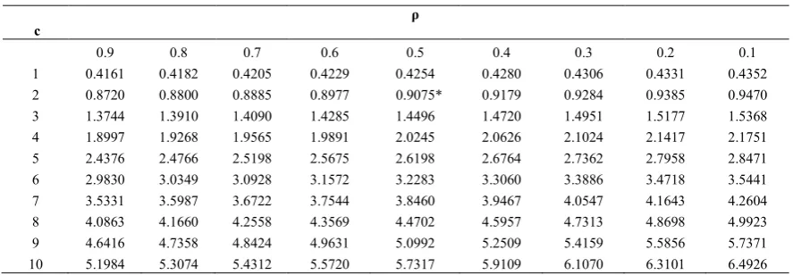
The procedure given in section 5 is used for constructing the mixed sampling plan indexed through AQL (
p
1). By assuming the probability of acceptance of the lot be
1 =0.95 and
1
=0.30, then p
2 1 values are calculated for differentvalues of c and ‘ρ’ using C program and is presented in Table 2.
Selection of the Plan
Table 2 is used to construct the plans when AQL (
p
1), ρ and care given. For any given values of
p
1 , c and ρ one candetermine n2 value using
n
2
n p
2 1/
p
1.Example 2: Given
p
1= 0.00763, ρ = 0.9, c = 4 and
1
= 0.30. Using Table 2, find2 2 1
/
1n
n p
p
= 1.8997 / 0.00763 = 410. For a fixed
1
= 0.30, the mixed sampling plan with SSP as attribute plan is n2 =410, ρ = 0.9 and c = 4.
Comparison of Mixed Sampling Plan indexed through MAPD and AQL
In this section MSP indexed through MAPD is compared with MSP indexed through AQL by fixing the parameters c and
j
. For the specified values of ρ, MAPD and MAAOQ with the assumption for
*
0.30 one can find the values of c and n2indexed through MAPD. By fixing the values of c and n2,find
the value of
p
1 by equatingP p
a( )
=
1 =0.95. For1
0.30
, c and n2 one can find the values of n2 using2 1 2
1
n p
n
p
from Table 2. For different combinations of ρ,MAPD and MAAOQ the values of c and n2 (indexed through
MAPD) and c and n2 (indexed through AQL) are calculated
and presented in Table 3.
Table 3 Comparison of plans
Given values Indexed Through
MAPD
Indexed Through AQL
MAPD MAAOQ ρ n2 c n2 c 0.022* 0.012 0.9 218 4 410 4 0.072 0.030 0.8 130 7 146 7 0.038 0.020 0.6 40 1 50 1 0.028 0.010 0.5 121 2 144 2
* OC curves are drawn
Construction of OC curve
The OC curves for the plans n2 = 218, c = 4, ρ = 0.9 (indexed
through MAPD) and n2 = 410, c = 4, ρ = 0.9 (indexed through
AQL) based on the different values of
n p
2 andP p
a
are presented in Figure 1.Figure 1 OC curves for SSP (218, 4) and (410, 4)
0 0.2 0.4 0.6 0.8 1
0 0.02 0.04 0.06 0.08 0.1
Pro
babil
ity
of
ac
ce
pt
a
nce
Product quality proportion defective
MAP D AQL
Table 2 n2AQL values for different values of ρ and c when
1= 0.95 and
1
= 0.30c
ρ
0.9 0.8 0.7 0.6 0.5 0.4 0.3 0.2 0.1
CONCLUSION
In this paper construction of mixed sampling plan as attribute plan indexed through MAPD and AQL are presented by taking IRPD as a baseline distribution. Further the plan indexed through MAPD is compared with the plan indexed through AQL. It is concluded from the study that the second stage sample size required for SSP indexed through MAPD is less than that of the second stage sample size of the SSP indexed through AQL. If the floor engineers know the levels of MAPD or AQL, they can have their sampling plans on the floor itself by referring to the tables. This provides the flexibility to the floor engineers in deciding their sampling plans. Various plans can also constructed to make the system user friendly by changing the first stage probabilities (
*
,
1
) and can also be compared for their efficiency.References
1. Bowker AH and Goode HP. “Sampling Inspection by Variables”, McGrawHill, Newyork. 1952.
2. Devaarul, S. “Certain Studies Relating to Mixed Sampling Plans and Reliability Based Sampling Plans”, Ph.D., Dissertation, Bharathiar University, Coimbatore, 2003, Tamil Nadu, India.
3. Mayer, P.L. A note on sum of Poisson probabilities and an application, Annals of Institute of Statistical Mathematics, 1967, Vol.19, pp.537-542.
4. Radhakrishnan, R. “Contribution to the study on Selection of Certain Acceptance Sampling Plans”, Ph.D., Dissertation, Bharathiar University, 2002, Tamilnadu, India.
5. Radhakrishnan, R. and Sekkizhar, J. Construction of sampling plans using intervened random effect Poisson distribution. The International Journal of Statistics and Management Systems, 2007a, Vol.2, 1-2, pp 88-97. 6. Radhakrishnan, R. and Sekkizhar, J. Construction of
conditional double sampling plans using intervened random effect Poisson distribution, Proceedings volume of SJYSDNS-2005, Acharya Nagarjuna University, Guntur. 2007b, Pp.57-61.
7. Radhakrishnan, R. and Sekkizhar, J. Application of intervened random effect Poisson distribution in process control plans, International Journal of Statistics and Systems. 2007c, Vol. 2. No.1. pp.29-39.
8. Sampath Kumar, R. Construction and Selection of Mixed Variables – Attributes Sampling Plans, Ph.D., Dissertation, Bharathiar University, Coimbatore, 2007, Tamil Nadu, India.
9. Sampath Kumar, R., Indra, M., and Radhakrishnan, R. Selection of mixed sampling plans with QSS-1(n;cN,cT)
plan as attribute plan indexed through MAPD and AQL ,
Indian Journal of Science and Techology, 2012c, Vol.5,No.2,Feb 2012, pp. 2096- 2099.
10. Sampath Kumar, R., Kiruthika, R., and Radhakrishnan, R. Construction of mixed sampling plans indexed through MAPD and LQL with Double sampling plan as attribute plan using Weighted Poisson distribution,
International Journal of Electronics and
Communication Engineering, 2012, Vol.5, No.3, pp. 39-47.
11. Sampath Kumar, R., Sumithra,S., and Radhakrishnan, R. Selection of mixed sampling plan with chsp-1 plan as attribute plan indexed through MAPD and MAAOQ,
International Journal of Applied Computational Science and Mathematics, 2012, Vol.1, No.1, pp. 37- 44. 12. Sampath Kumar, R., Vijayakumar, R. and Radhakrishnan, R. Selection of Mixed Sampling plan using Intervened Random effect Poisson distribution.
International Journal of Recent Scientific Research (IJRSR), August 2012, Vol. 3, Issue, 8, pp.703-707, 13. Sampath Kumar, R., Vijayakumar, R. and
Radhakrishnan, R. Selection of Mixed Sampling plan with Repetitive Group Sampling Plan as Attribute Plan Indexed through MAPD and IQL using IRPD.
International Journal of Computer Information Systems (IJCIS), 2012, Vol.4, Number 5, May 2012. ISSN: 2229 – 5208.
14. Schilling, E.G. A General Method for Determining the Operating Charateristics of Mixed Variables – Attribute Sampling Plans Single Side Specifications, S.D. known, Ph.D Dissertation – Rutgers – The State University, New Brunswick, New Jersy, 1967.
15. Shanmugam, R. An intervened Poisson distribution and its medical applications, Biometrics, 1985, 41, 1025-1029.
16. Soundararajan, V. Maximum allowable percent defective (MAPD) single sampling inspection by attributes plan, Journal of Quality Technology, 1975, Vol.7, No.4, pp.173-182.
How to cite this article:
Vijaya Kumar R and Sampath Kumar R.2019, Construction of Mixed Sampling Plan With Single Sampling Plan As Attribute Plan Indexed Through MAPD And AQL Using IRPD. Int J Recent Sci Res. 10(08), pp. 34113-34117.
DOI: http://dx.doi.org/10.24327/ijrsr.2019.1008.3823