Sparse Spectrotemporal Coding of Sounds
David J. Klein
Institute of Neuroinformatics, University of Zurich and ETH Zurich, Winterthurerstrasse 190, CH-8057 Zurich, Switzerland Email:[email protected]
Peter K ¨onig
Institute of Neuroinformatics, University of Zurich and ETH Zurich, Winterthurerstrasse 190, CH-8057 Zurich, Switzerland Email:[email protected]
Konrad P. K ¨ording
Institute of Neurology, University College London, Queen square, London, WC1N 3BG, UK Email:[email protected]
Received 1 May 2002 and in revised form 28 January 2003
Recent studies of biological auditory processing have revealed that sophisticated spectrotemporal analyses are performed by central auditory systems of various animals. The analysis is typically well matched with the statistics of relevant natural sounds, suggest-ing that it produces an optimal representation of the animal’s acoustic biotope. We address this topic ussuggest-ing simulated neurons that learn an optimal representation of a speech corpus. As input, the neurons receive a spectrographic representation of sound produced by a peripheral auditory model. The output representation is deemed optimal when the responses of the neurons are maximally sparse. Following optimization, the simulated neurons are similar to real neurons in many respects. Most notably, a given neuron only analyzes the input over a localized region of time and frequency. In addition, multiple subregions either excite or inhibit the neuron, together producing selectivity to spectral and temporal modulation patterns. This suggests that the brain’s solution is particularly well suited for coding natural sound; therefore, it may prove useful in the design of new computational methods for processing speech.
Keywords and phrases:sparse coding, natural sounds, spectrotemporal receptive fields, spectral representation of speech.
1. INTRODUCTION
The brain evolves both overindividual and overevolutionary timescales embedded into the properties of the real world. It thus seems that the properties of any sensory system should be matched with the statistics of the natural stimuli it is typi-cally operating on [1]. This would suggest that the function-ality of sensory neurons can be understood in terms of cod-ing optimally for natural stimuli.
This line of inquiry has been fruitful in the visual modal-ity. Many properties of the mammalian visual system can be explained as leading to optimally sparse neural responses in response to pictures of natural scenes. Within this paradigm, it is possible to reproduce the properties of neurons in the lateral geniculate nucleus (LGN) [2] and of simple cells in the primary visual cortex [3, 4, 5]. The term “sparse representation” is often used in these studies to address one of two distinct albeit related meanings: (1) neurons of the population should have significantly distinct function-ality in order to avoid redundancy, and (2) the neurons
should exhibit sparse activity over time such that their ac-tivity level is often close to zero, but is occasionally very high.
A large number of independent component analysis (ICA) (cf. [6,7]) studies also effectively use this principle and demonstrate the computational advantages of such a repre-sentation.
interest since the right type of sound representation might be a key to improved recognition of natural language, speech denoising, or speech generation.
2. METHODS
Inputs
Narratives from 29 distinct languages, taken from the lan-guage illustrations in part 2 of the handbook of the Interna-tional Phonetic Association (IPA) (available athttp://www2. arts.gla.ac.uk/IPA/sndfiles.html), were preprocessed by sim-ulated peripheral auditory neurons [11,12] using the “NSL Tools” Matlab package (courtesy of the Neural Systems Lab-oratory, University of Maryland, College Park, available at http://www.isr.umd.edu/CAAR/pubs.html). This peripheral analysis employs constant-Q bandpass frequency analysis similar to that of the mammalian cochlea including high-frequency preemphasis (first-order highpass, corner fre-quency of 300 Hz), followed by nonlinear (sigmoidal) trans-duction, and half-wave rectification and smoothing (first-order lowpass, corner frequency of 100 Hz) for envelope ex-traction. As a comparison, we obtained a second dataset by recording audio data from one voluntary human sub-ject (KPK) reading German-language texts, using a standard microphone (Escom) and Cool Edit Pro software (Syntril-lium Software, Phoenix, USA) recording mono at 44 kbit, 16 bits precision (Figure 1a). The resulting data can be viewed as spectrograms, which represent the time-dependent spec-tral energy of sound. An example is shown in Figures1a and 1b, which show, respectively, the input and output of the pe-ripheral model to the utterance “Komm sofort nach Hause” (“come home right away” in German).
The spectrograms have 64 points along the tonotopic (spectral) axis, covering a frequency range from 185 to 7246 Hz. This corresponds to a spectral resolution of approx-imately 12 channels per octave. Temporally, the data is ar-ranged into overlapping blocks of 25 points, each covering 250 milliseconds. One block of data is taken per 10 millisec-onds. The data is subjected to a principal component anal-ysis (PCA), and the first 200 components are set to have unit variance (called whitening) and are subsequently used as input vectors I(t) of length 200 to the optimization al-gorithm. Thirty thousand subsequent samples are used as input.
Neuron model
Hundred neurons are simulated, each of which has a weight vectorWiof length 200. The activitiesAiof the neurons are defined as follows:
Ai(t)=ϑI(t)Wi, (1)
where ϑ is the heavyside function: ϑ(x) = x for x > 0, ϑ=0 otherwise. The neurons are thus characterized by linear threshold properties. The parameters of the simulated neu-rons are optimized by a fast optimization algorithm, called resilient backprop [13], to maximize the following objective
function:
where ∗ denotes the average over all stimuli and Ai is the activity of the neuron. The simulated neurons, further-more, should not all have the same properties; they should be decorrelated. We thus add a second term
Ψdecorr= −
where CC denotes the coefficient of covariation and std is the standard deviation. The first term biases the neurons to have distinct activity patterns, while the latter term effectively normalizes the standard deviation. The optimization is per-formed in principal component space (cf. [14]) for the sake of faster computation. This transformation is done using the Matlab princomp routine.
Analysis
The optimized spectrotemporal analysis performed by the neurons is characterized by the corresponding STRF accord-ing to the learned set of optimal weights. Properties of that STRFs are measured in a manner similar to that used in neurophysiological studies. The best frequency (BF) and best time (BT) are defined as the spectral and temporal locations, respectively, of the maximum weight. The−10 dB excitatory-tuning bandwidth and duration are defined as the spectral and temporal extent of the portion of the STRF within 1/√10 of the peak value.
In addition, properties of the two-dimensional Fourier transform of the STRFs are measured. Here, the spectral and temporal filtering of the input signal is quantified by the peak and cutoff (−10 dB) frequencies of the Fourier transform, along both the spectral and temporal axes. In addition, the extent to which an STRF encodes frequency modulation of a given direction is quantified by a directionality index. This index is computed as the relative power difference of the first two quadrants of the Fourier transform, which lies between −1 and 1.
It is illuminating to compare the properties of the op-timized network with the statistics of the employed stim-ulus ensemble. The output of the peripheral auditory pro-cessing was thus subjected to a multiscale two-dimensional wavelet (second-derivative Gaussian) analysis [15], from which the energy distribution of temporal and spectral mod-ulations, as a function of tonotopic position, was com-puted.
3. RESULTS
3.1. Data properties
Komm so- fort nach Hau- se
Time [ms]
1500 0
(a)
Model of early auditory processing
0 1500
Time [ms] 250
1000 4000
F
requency
[Hz]
Segments 250 ms
0 250
250 1000 4000
F
requency
[Hz]
Time [ms] (b)
· · ·
1 2 3 4 5
6 7 8 9
· · ·
Time [ms] 0 250
250 1000 4000
F
requency
[Hz]
Preprocesses input to Network
(c)
Figure 1: Methods. (a) Recorded speech data are shown as raw waveforms. (b) This data is input to a model of the auditory system’s early stages resulting in a spectrogram, where the strength of the activity is color-coded. These spectrograms are subsequently cut into overlapping pieces of length 250 milliseconds for each. The principal components of this PCA are shown in (c), color-coded in a scale where blue represents small values and red represents large values.
for learning effectively low-passes the stimuli; however, the first 200 components that are used for learning account for more than 90% of the total variance of the data. We previ-ously reported that the form of the lowest components is also robust to changes of the spectrotemporal resolution of the peripheral auditory model [16].
A
Figure2: Results from optimising sparseness. Representative color-coded STRFs of the neurons are shown. The same STRF is often seen at different delays. In this case only the one with most energy in the middle of the STRF is shown.
3.2. Receptive field properties
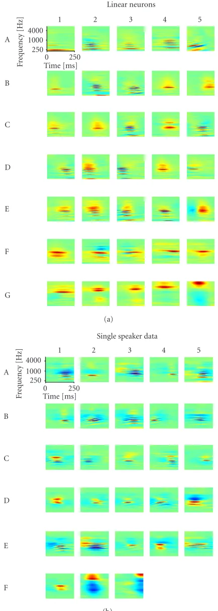
The employed IPA speech database contains both male and female speakers from a variety of languages. Representative-learned filters for optimal spectrotemporal encoding of this dataset are illustrated in Figure 2. Here, STRFs of linear-threshold neurons were obtained by optimizing the sparse-ness of the neurons’ stimulus-evoked activity.
A number of important properties can be observed for these STRFs. First of all, the STRFs are typically well-localized in time and in spectrum. Secondly, many of the STRFs exhibit multiple peaks and troughs in the form of dampened oscillations along the spectral and temporal axes. Finally, a range of frequency modulations are seen in the STRFs; these are evidenced by oblique orientations of the STRFs (e.g., see neurons B1 and E4). It should be noted that all these three properties are also exhibited in STRFs obtained from neurophysiological experiments.
The specific manifestation of these three properties how-ever varies from neuron to neuron. For instance, different STRFs are centered on different regions of the spectrotem-poral plane and have different spectral and temporal extents. The distribution of the position and shape parameters for the
entire population of STRFs is shown inFigure 3a. For clarity, the sizes of the iconified STRFs have been reduced to 1/8 of their actual values.
In addition, the frequency of the spectral and temporal oscillations exhibited in the STRFs and the amount of damp-ening varies across the population, as shown in Figures 3b and3c. In the Fourier domain, these two properties conspire to produce selectivity for specific modulations along the tem-poral or the spectral axis.Figure 3bquantifies this selectivity for the spectral domain and shows how the spectral charac-teristics of the Fourier transform vary as a function of the tonotopic position of the STRF. For about half of the STRFs, the peak of the Fourier transform lies between about 0 and 1 cycle per octave (c/o), and the upper cutofflies between 1 and 3 c/o. A radically different strategy is seen at low frequencies. Here, many neurons pass significantly higher spectral mod-ulations, ranging from 2 to 6 c/o. This is most likely due to the presence of low-frequency high-scale harmonic patterns in the speech input. Indeed,Figure 3dshows that the stimu-lus itself contains a high proportion of high-scale energy at low frequencies.
The situation is somewhat different in the temporal do-main. In general, the STRFs are highly damped in the tem-poral direction, producing temtem-poral modulation selectivity that is generally lowpass. This fact is evident in Figure 3e which shows that the peak of the Fourier transform never rises above 2 Hz; furthermore, the cutoff frequency is in-versely correlated with the temporal width of the STRF and never rises above 10 Hz. Nevertheless, the range of tempo-ral frequencies present in the STRFs is largely consistent with the average temporal composition of the speech input which has a majority of its power concentrated below 10 Hz (Figure 3f).
Finally, different STRFs exhibit different degrees of fre-quency modulation, as quantified by the direction selectiv-ity index (Figure 3g). This index is−1 if an STRF exhibits solely positive-going frequency modulations, is 1 for solely negative-going frequency modulations, and is 0 for equal amounts of positive and negative frequency modulation. The population distribution is unimodal and peaks at an index of 0, which is similar to that obtained from neurophysiological experiments [8].
0 250
Temp. mod. freq. [Hz] 0
Figure3: Quantitative properties. (a) The time-frequency tiling properties of the neurons are shown. The center of each ellipse represents the BF and BT of a neuron. The vertical and horizontal extent of the ellipse represents 1/8 of the width of the STRF in the direction of time and spectrum. The factor of 1/8 was introduced to improve visibility of the data. (b) Both the peak (blue) and the high-frequency cutoff (red) of the frequency of spectral modulation are plotted as a function of the best frequency of the neuron. (c) The spectral width of the STRF (red) of the excitatory subregion (blue) is plotted as a function of the BF of the neuron. (d) The IPA stimuli are analyzed in the Fourier domain. The mean of the absolute values of the wavelet transforms of spectrograms taken from the IPA database are shown. (e) Both the peak (blue) and the high-frequency cutoff(red) of the frequency of temporal modulation are plotted as a function of the temporal width of the neuron. (f) The normalized power is shown as a function of the temporal modulation frequency. (g) The index for direction selectivity is calculated and its histogram is shown.
3.3. Dependence on the neuron model
The current study has so far focused upon STRFs which produce optimally sparse activity in linear-threshold
in previous simulations [16]. In order to compare the re-sults, we repeated the current simulation using purely lin-ear neurons. Representative results are shown in Figure 4a. Qualitatively speaking, the major features of the neurons’ STRFs remain conserved. However, the spectral and tem-poral extents of the STRFs are typically somewhat larger, and, furthermore, the presence of negative deflections is somewhat reduced. The combination of these two prop-erties produce a spectrotemporal analysis that is more re-stricted to low spectral and temporal modulation frequen-cies.
3.4. Dependence on the dataset
For the sake of comparison, the simulations with linear-threshold neurons were repeated with a different speech in-put, this time obtained from a single speaker (seeSection 2). Sparseness requires that the neurons should occasionally have very high activity while having small activities most of the time. If we only have one speaker, they can thus be expected to distinguish specific elements of the speaker’s speech rather than distinguishing utterances from different speakers. The results are likely not to generalize well to ut-terances of other speakers while being optimal for utter-ances of the speaker. Figure 4b shows the learned recep-tive fields. Far more of the neurons code for changes of the pitch of the sounds. A number of them even code for compound features (e.g., neuron D4) where some frequen-cies rise while others fall. Thus the dataset used clearly in-fluences the data and, therefore, must be carefully consid-ered.
3.5. Dependence on the number of principal
components used
The number of principal components used to encode the in-put potentially has some influence on the resulting receptive fields. Low-order principal components tend to be of lower frequency than higher frequency components, and so using fewer principal components has an effect similar to selec-tively reducing the resolution of the peripheral spectrotem-poral analysis. To test the influence of this effective smooth-ing, the simulations were repeated using reduced numbers of principal components. Even if only 25 components are used (Figure 5), the typical STRF properties described above still apply. This includes even the encoding of low-frequency fine-scale spectral features due to voice pitch. Thus the number of principal components only has a limited influence on the re-sulting STRFs.
4. DISCUSSION
When analyzing the computational properties of neural sys-tems, it is of central importance to have a thorough under-standing of the input representation. A number of other the-oretical studies of optimal auditory processing have used raw acoustic-pressure waveforms as input representation. For ex-ample, Bell [17] studied the learning of auditory temporal filters using ICA, and Lewicki and Sejnowski [18] showed that using overcomplete representations can significantly
A
B
C
D
E
F
G
1 2 3 4 5
Linear neurons
0 250
Time [ms] 250
1000 4000
F
requency
[Hz]
(a)
A
B
C
D
E
F
1 2 3 4 5
Single speaker data
0 250
Time [ms] 250
1000 4000
F
requency
[Hz]
(b)
A
Figure 5: Dependence on the number of principal components. The representative STRFs are shown for a simulation where a smaller number of principal components were used. (a) shows the results from using 25 components and (b) shows the results from using 100 components.
improve the model quality. Using a balanced dataset taken from various sound sources, it was possible to approximately reproduce the spectral analysis performed by the peripheral auditory system [19].
How do central auditory neurons combine the features already encoded by more peripheral neurons? Recent neu-rophysiological studies in various species have shown that the central auditory system jointly processes the spectral and temporal characteristics of sound in a dazzling variety of ways [8, 9, 20, 21, 22]. The current study strives to pro-vide a method for speculation on the functionality of such processes. In doing so, the raw waveforms are first prepro-cessed using an auditory peripheral model. This produces a spectrogram-like representation of sound, which is bet-ter suited for describing the information-bearing elements of natural sounds such as speech [23]. Furthermore, since cen-tral auditory neurons display largely linear processing of the spectrotemporal envelope of sound [8,24], it increases the likelihood that this style of inquiry will be fruitful. In fact, the results obtained from spectrogram inputs exhibit many of the rich properties of real auditory neurons.
We used PCA to preprocess the spectrogram before feed-ing it into the sparse codfeed-ing algorithm. The resultfeed-ing com-ponents capture prominent statistical properties of the data. For example, their banded structure at low frequencies re-flects the dominant influence of voice pitch. It is possible that this preprocessing will strongly influence the resulting STRFs. However, one can argue against this likelihood on analytical grounds. Assume the number of principal com-ponents used is identical to the number of input samples in each spectrogram. The transformation to the principal com-ponent space is then an orthonormal matrix of full rank. Be-cause this matrix can be inverted, each local optimum of the method in PCA space is also an optimum to the method in input space. The chosen principal components can thus be expected to be of minor influence on the resulting STRFs— provided that enough principal components are used. Our simulations showed that 100 components, or perhaps even fewer, are enough. Note also that it is possible (albeit nu-merically very expensive) to perform the simulations with-out PCA preprocessing, and doing so results in similar STRFs (data not shown).
STRFs in the auditory system show some functional sim-ilarity to spatiotemporal receptive fields in the visual system. Many properties of visual neurons have been successfully learned by maximizing sparseness [25]; it has even been pos-sible to quantitatively compare the properties of the visual system with the properties of simulated neurons, (e.g., [4]). This study extends such methods to auditory data. How-ever, while our simulations are able to qualitatively repro-duce many important properties of neurons in AI, a thor-ough quantitative comparison of properties remains an im-portant problem for further research. In doing so, it will first be necessary to assemble a rich database of sounds that accurately represents an animal’s acoustic biotope. One must then devise a compact learning mechanism that leads to neuronal properties that closely correspond to those ob-served experimentally. This might even necessitate the devel-opment of novel algorithms for learning nonlinear neuronal properties.
prediction. During an animal’s development, one should be able to manipulate the sparseness statistics of the acous-tic environment, such that the neurophysiological proper-ties of neurons are altered. For example, raising an animal in an auditory environment where a certain frequency band is sparser than another should enhance the neural repre-sentation of the sparse frequencies. Furthermore, one might facilitate auditory learning by making the underlying audi-tory features more sparse. In fact, the training procedures for children demonstrated in [26] can be interpreted in this framework.
In the visual modality, the sparse representation of im-ages enabled new computational approaches which lead to powerful algorithms for image denoising [7], image com-pression [27], and preprocessing for image recognition. This suggests that using sparse coding on spectrotemporal data might well lead to better algorithms for the denoising of speech, for the compression of auditory data, and for the recognition of natural language.
ACKNOWLEDGMENTS
We want to thank the Swiss National Science Founda-tion (SNF), Swiss Priority Programs (SPP), Collegium Hel-veticum (KPK), the Swiss National Fonds (PK) Grant no. 3100-51059.97), and the EU AMOUSE project (KPK and PK). We would like to thank the ADA—“the Intelligent Room” Project that is part of EXPO 2002, which partially pays DJK and in part inspired this project. We would like to thank Bruno Olshausen, Tony Bell, and Heather Read for in-spiring discussions and technical assistance.
REFERENCES
[1] H. B. Barlow, “Possible principles underlying the transforma-tions of sensory messages,” inSensory Communication, W. A. Rosenblith, Ed., pp. 217–234, MIT Press, Cambridge, Mass, USA, 1961.
[2] J. J. Atick, “Could information theory provide an ecological theory of sensory processing?,”Network: Computation in Neu-ral Systems, vol. 3, no. 2, pp. 213–251, 1992.
[3] B. A. Olshausen and D. J. Field, “Emergence of simple-cell receptive field properties by learning a sparse code for natural images,”Nature, vol. 381, no. 6583, pp. 607–609, 1996. [4] J. H. van Hateren and A. van der Schaaf, “Independent
com-ponent filters of natural images compared with simple cells in primary visual cortex,” Proc. R. Soc. Lond. B, vol. 265, pp. 359–366, November 1998.
[5] A. J. Bell and T. J. Sejnowski, “The ”independent compo-nents” of natural scenes are edge filters,”Vision Research, vol. 37, no. 23, pp. 3327–3338, 1997.
[6] P. Comon, “Independent component analysis,” inProc. Int. Sig. Proc. Workshop on Higher-Order Statistics, J. L. Lacoume, Ed., Chamrousse, France, July 1991.
[7] A. Hyv¨arinen, “Sparse code shrinkage: Denoising of nongaus-sian data by maximum likelihood estimation,” Neural Com-putation, vol. 11, no. 7, pp. 1739–1768, 1999.
[8] D. A. Depireux, J. Z. Simon, D. J. Klein, and S. A. Shamma, “Spectro-temporal response field characterization with
dy-namic ripples in ferret primary auditory cortex,” Journal of Neurophysiology, vol. 85, no. 3, pp. 1220–1234, 2001. [9] R. C. deCharms, D. T. Blake, and M. M. Merzenich,
“Opti-mizing sound features for cortical neurons,”Science, vol. 280, pp. 1439–1444, 1998.
[10] S. A. Shamma, “On the role of space and time in auditory processing,”Trends in Cognitive Sciences, vol. 5, no. 8, pp. 340– 348, 2001.
[11] X. Yang, K. Wang, and S. A. Shamma, “Auditory representa-tions of acoustic signals,” IEEE Transactions on Information Theory, vol. 38, no. 2, pp. 824–839, 1992.
[12] K. Wang and S. A. Shamma, “Spectral shape analysis in the central auditory system,” IEEE Trans. Speech and Audio Pro-cessing, vol. 3, pp. 382–395, 1995.
[13] M. Riedmiller and H. Braun, “A direct adaptive method for faster backpropagation learning: The RPROP algorithm,” inProc. IEEE International Conference on Neural Networks, H. Ruspini, Ed., pp. 586–591, San Francisco, Calif, USA, March 1993.
[14] A. Hyv¨arinen, “Survey on independent component analysis,” Neural Computing Surveys, vol. 2, pp. 94–128, 1999.
[15] T. Chi, Y. Gao, M. C. Guyton, P. Ru, and S. A. Shamma, “Spectro-temporal modulation transfer functions and speech intelligibility,”Journal of the Acoustical Society of America, vol. 106, no. 5, pp. 2719–2732, 1999.
[16] K. P. K¨ording, P. K¨onig, and D. J. Klein, “Learning of sparse auditory receptive fields,” inProc. International Joint Confer-ence on Neural Networks, Honolulu, Hawaii, USA, May 2002. [17] A. J. Bell and T. J. Sejnowski, “Learning the higher-order
structure of a natural sound,”Network: Computation in Neu-ral Systems, vol. 7, no. 2, pp. 261–266, 1996.
[18] M. S. Lewicki and T. J. Sejnowski, “Learning overcomplete representations,”Neural Computation, vol. 12, no. 2, pp. 337– 365, 2000.
[19] M. S. Lewicki, “Efficient coding of natural sounds,” Nature Neuroscience, vol. 5, no. 4, pp. 356–363, 2002.
[20] L. M. Miller, M. A. Escab´ı, H. L. Read, and C. E. Schreiner, “Spectrotemporal receptive fields in the lemniscal auditory thalamus and cortex,”Journal of Neurophysiology, vol. 87, no. 1, pp. 516–527, 2002.
[21] K. Sen, F. E. Theunissen, and A. J. Doupe, “Feature analysis of natural sounds in the songbird auditory forebrain,”Journal of Neurophysiology, vol. 86, no. 3, pp. 1445–1458, 2001. [22] J. J. Eggermont, “Wiener and Volterra analyses applied to the
auditory system,” Hearing Research, vol. 66, no. 2, pp. 177– 201, 1993.
[23] L. Cohen,Time-Frequency Analysis, Prentice Hall, Englewood Cliffs, NJ, USA, 1995.
[24] N. Kowalski, D. A. Depireux, and S. A. Shamma, “Analysis of dynamic spectra in ferret primary auditory cortex. II. Predic-tion of unit responses to arbitrary dynamic spectra,” Journal of Neurophysiology, vol. 76, no. 5, pp. 3524–3534, 1996. [25] B. A. Olshausen, “Sparse codes and spikes,” inProbabilistic
Models of the Brain: Perception and Neural Function, R. P. N. Rao, B. A. Olshausen, and M. S. Lewicki, Eds., MIT Press, Cambridge, Mass, USA, 2001.
[26] M. M. Merzenich, W. M. Jenkins, P. Johnson, C. Schreiner, S. L. Miller, and P. Tallal, “Temporal processing deficits of language-learning impaired children ameliorated by train-ing,”Science, vol. 271, no. 5245, pp. 77–81, 1996.
David J. Kleinwas born in Florida (USA) in 1972. His undergraduate and graduate education in electrical engineering was ob-tained from the Georgia Institute of Tech-nology (Atlanta, Georgia) and the Univer-sity of Maryland (College Park, Maryland), respectively. He is currently working as a Visiting Scientist at the Institute of Neu-roinformatics (University/ETH Z¨urich) in Z¨urich, Switzerland, where he is developing
models of auditory cortical function and investigating the useful-ness of auditory neuroscientific knowledge for various acoustical signal processing applications, including sound recognition, pitch extraction, and sound localization.
Peter K¨onigstudied physics and medicine at the University of Bonn, Bonn, Germany. He was with the Department of Neurophys-iology at the Max Planck Institute for Brain Research, Frankfurt, Germany, where he re-ceived the Habilitation degree in 1990. Af-ter working as a Senior Fellow at the Neu-rosciences Institute in San Diego, Calif, he joined the Institute of Neuroinformatics, Z¨urich, Switzerland, in 1997. Here, he is
us-ing experimental and theoretical approaches to study the mam-malian visual system, with a particular interest in the processing of natural stimuli.
Konrad P. K¨ordingwas born in Darmstadt, Germany, in 1973. He studied Physics in Heidelberg and Z¨urich. He got his Ph.D. degree from ETH Z¨urich addressing opti-mality in the visual system. He worked on biophysical modelling of single cells, oscilla-tory network dynamics of spiking neurons. More recently, he worked on learning rules that replicate the properties of visual neu-rons when trained on natural stimuli. His