R E S E A R C H
Open Access
Multiple descriptions for packetized
predictive control
Jan Østergaard
1*and Daniel Quevedo
2Abstract
In this paper, we propose to use multiple descriptions (MDs) to achieve a high degree of robustness towards random packet delays and erasures in networked control systems. In particular, we consider the scenario, where a data-rate limited channel is located between the controller and the plant input. This forward channel also introduces random delays and dropouts. The feedback channel from the plant output to the controller is assumed noiseless. We show how to design MDs for packetized predicted control (PPC) in order to enhance the robustness. In the proposed scheme, a quantized control vector with future tentative control signals is transmitted to the plant at each discrete time instant. This control vector is then transformed into M redundant descriptions (packets) such that when receiving any 1≤J≤Mpackets, the current control signal as well asJ−1 future control signals can be reliably reconstructed at the plant side. For the particular case of LTI plant models and i.i.d. channels, we show that the overall system forms a Markov jump linear system. We provide conditions for mean square stability and derive upper bounds on the operational bit rate of the quantizer to guarantee a desired performance level. Simulations reveal that a significant gain over conventional PPC can be achieved when combining PPC with suitably designed MDs.
Keywords: Quantization, Networked control, Multiple descriptions
1 Introduction
In networked control systems (NCSs), the controller com-municates with the plant via a general purpose communi-cation network [1, 2]. When compared to using dedicated hardwired control networks, the use of general purpose and possibly wireless communication technology brings significant benefits in terms of efficiency, interoperability, deployment costs, etc. However, the use of practical com-munication technology also leads to new challenges, since the network needs to be taken into account in the overall design, see also [1–7].
In this paper, we will focus on the existence of a dig-ital network between the controller and the plant input. This network contains either a single channel that intro-duces i.i.d. packet delays and erasures or multiple inde-pendent channels with i.i.d. packet delays and erasures. The channel between the plant output and the controller is considered ideal, i.e., noiseless and instantaneous. For example, this could be a situation where the controller
*Correspondence: [email protected]
1Department of Electronic Systems, Aalborg University, Fredrik Bajers Vej 7b, Aalborg, Denmark
Full list of author information is available at the end of the article
and plant communicates over wireless channels. The con-troller could be battery driven and therefore with limited transmission power. On the other hand, the plant might not have a limitation on the transmission power. In this case, the reverse channel from the plant to the con-troller has a significantly greater SNR than the forward channel between the controller and the plant. There are many other practical sitations with wireless controller-actuator links but direct sensor-controller connections, e.g., groups of agents/vehicles/robots/drones. Their posi-tions/formation are sensed via a system comprising a camera and attached controller. Activation commands are then sent wirelessly to the agents.
The main contributions of this work is the theoretical analysis and practical design of the quantized control sig-nals. In particular, we propose to combine a recent robust control strategy known as (quantized) packet predictive control (PPC) [8–11] with a joint source-channel cod-ing strategy based on multiple description (MD) codcod-ing [12, 13]. We provide computable upper bounds on the operational bit rate required for coding the quantized con-trol signals (descriptions) and provide a practical design based on our theoretical analysis. The simulation study
shows that the combination of MDs and PPC provides a significant improvement over PPC in the case of large packet loss ratios.
In quantized PPC, a control vector with the current and N −1 future predicted plant inputs is constructed at the controller side to compensate for random delays and packet dropouts in the channel. Thus, in the case of packet erasures (and if not too many consecutive dropouts occur), the buffer will feed the plant with the appropri-ate future predicted control value [8]. The key principle of MDs is to encode a source signal into a number of descriptions (packets) that are transmitted over separate channels. Each description is able to approximate the source signal to within a prescribed quality. Moreover, if several descriptions are received, they can be combined to further improve the reconstruction quality. Thus, in the case of packet erasures, it is possible to achieve a graceful degradation of the reconstruction quality [13].
The design of optimal quantized control strategies sub-ject to data rate limitations defines a complicated problem that lies in the intersection of signal processing and con-trols. In particular, if the quantizers are designed using conventional open-loop source-coding strategies, it can-not be guaranteed that the overall system will be stable, when used in closed-loop control. Indeed, the resulting data rate could exceed the bandwidth of the digital chan-nel, the data rate could be too low to capture the plant uncertainty and thereby not guarantee stability, or the non-linear effects due to quantization could have a nega-tive impact on the overall stability when fed back into the system [8, 9, 14, 15].
The combination of MDs and PPC has to the best of the authors’ knowledge not been considered before (except in the conference contributions of the authors [16–18]). In [16], MDs were used for power control in wireless sensor networks. The quantizers were designed under high-resolution assumptions, and no stability assessment was provided. In [17, 18], the preliminary ideas for the cur-rent work (without analysis and proofs) were presented. MDs for state-estimation was considered in [19, 20] under high-resolution quantization assumptions. The design of lattice quantizers for PPC without MDs was treated in [16, 21] for the cases of entropy-constrained and resolution-constrained quantization, respectively.
In this work, we will focus on LTI plant models, which are (possibly) open-loop unstable. Thus, it is necessary to provide quantized control signals to the plant in a reli-able way to guarantee stability in the presence of data rate limitations, random packet delays and erasures. Our key idea is to design and use MDs in a novel way that dif-fers from how it is traditionally used. Traditionally, when the received descriptions are combined at the decoder, the approximation of a given source signal is improved. On the other hand, in the proposed work, when the
received descriptions are combined at the decoder, then rather than improving existing control signals, new future controls signals are instead recovered.
There exists a vast amount on literature on MJLS with delays, cf.,[22–25]. In the present work, we show that the overall system with delays, erasures, quantization effects, and multiple descriptions, can be cast as a Markov jump linear system (MJLS), which makes it possible to use general stability results from the MJLS literature [26, 27].
The paper is organized as follows. Section 2 contains background information on quantized PPC. Section 3 contains the system analysis of a theoretical joint PPC and MD scheme. Section 4 presents the design of the com-bined practical PPC and MD scheme. Section 5 provides a simulation study of the proposed scheme. Section 6 con-tains the conclusions. Proofs of lemmas and theorems are deferred to the appendices.
1.1 Notation
LetS↓be the down-shift-by-one matrix operator, which replaces thejth row of anN×Mmatrix by its(j−1)th row forj = N,. . ., 2. Similarly, defineS↑ as the up-shift-by-one matrix operator. Leteidenote the unit-vector aligned with theith axis of the Cartesian coordinate system, e.g., e2 =[ 0, 1, 0,· · ·, 0]T, where the dimension of ei will be clear from the context. Let1i ∈ Ri be the all-ones vec-tor of dimensioni. Letγibe the matrix operator that takes theith diagonal of anN×N matrix, wherei = 1 is the main diagonal andi > 1 are diagonals above the main diagonal. Thus,γi(A)∈RN−i+1ifA∈RN×N. We will use
σr(A)to denote the spectral radius of the matrixA, and A⊗Bdenotes the usual Kronecker product between the matricesAandB. The squared and weightedl2-norm of a vector, sayx, is written asx2P=xTPx, whereP0, i.e., Pis a positive semidefinite matrix.
2 Quantized packetized control over erasure channels
In this section, we provide a summary of existing results on quantized PPC and relate them to the present situa-tion. The system considered is shown in Fig. 1. For a more detailed presentation of quantized PPC, see [11].
2.1 System model
We consider the following discrete-time stochastic lin-ear time invariant (LTI) possibly unstable dynamical plant with statext∈Rz,z≥1 and scalar inputut∈R:
xt+1=Axt+B1ut+B2wt, t∈N. (1)
In (1),wt ∈ Rz
Fig. 1System setup. The PPC communicates with the plant via a data-rate limited (digital) erasure channel with delays
Rz×z. We do not assume thatA ∈ Rz×z is stable; how-ever, we will assume that the pair(A,B1) is stabilizable. The initial statex0is arbitrarily distributed with bounded variance.
2.2 Cost function
In MPC, at each time instanttand for a given plant state xt, one often uses a linear quadratic cost function on the form [28]:
V(u¯,xt)xN2P+ N−1
=0
x2Q+λ(u)2, (2)
whereN ≥ 1 is the horizon length, and the design vari-ablesP 0,Q 0 and λ > 0 allow one to trade-off control performance versus control effort. The variables xandu¯ldenote tentative variables and are defined below. The final state weighting xN2P in (2) aids in stabiliz-ing the feedback loop by approximatstabiliz-ing the effect of the infinite-horizon behavour [28]. For example, one may choosePas the unique positive semidefinite solution to the discrete algebraic Riccati equation:
P=ATPA+Q−ATPB1
λ+BT1PB1
−1
BT1PA, (3)
which exists if the system (1) is stabilizable [28].
The cost function in (2) examines a prediction of the plant model over a finite horizon of lengthN. It is com-mon to assume that the predicted state trajectories at time t are independent of the buffer contents at the decoder (i.e., they are independent of what has been received at the plant input side), network effects, and the external disturbanceswt, and are generated by
x+1=Ax+B1u, (4)
x0 = xt, while the entries inu¯ = u0,. . .,uN−1T rep-resent the associated predicted plant inputs. Thus, the current control vector
¯
ut=[ut(1),. . .,ut(N)]T
contains the control signal ut(1) for the current time instanttas well asN−1 future predictive control signals for time up tot+N−1.
One may include the effect of the channel delays in the cost function (2) by, for example, formulating the indi-vidual stage costs in terms of their expected stage costs, i.e., weighting by the probabilities of control signals being delayed:
E N−1
=1
x2Q+λ(u)2= N−1
=1
x2Q+λ(u)2p, (5)
wherepdenotes the probability of using the control sig-nal u. Moreover, in this work, we will also model the effect of the quantizer directly in the design of the control signalu, see Section 2.4 for details.
Following the ideas underlying PPCs, see, e.g., [29], at each time instantt, and for current statext, the controller sends theentireoptimizing sequence,u¯t, to the actuator node. Depending upon future packet dropout scenarios, a subsequence ofu¯twill be applied at the plant input, or not. Following the receding horizon paradigm, at the next time instant, xt+1 is used to carry out another optimization, yieldingu¯t+1, etc.
2.3 Network effects
As illustrated in Fig. 1, we shall assume that the backward channel of the network is noiseless and instantaneous, whereas the forward channel is a packet erasure chan-nel, where packets can be delayed and also be received out-of-order. In fact, we allow the delay to be unbounded, which means that packets can be lost. In our setup, if a transmitted packet has not been received withinN con-secutive time slots, it is considered lost. In MD coding, it is common to assume the availability of eitherMseparate and independent channels or a single (compound) chan-nel where theMpackets can be sent simultaneously and yet be subject to independent erasures and delays [13]. Formally, we defineτti ∈ N0∪ ∞to be the delay experi-enced by theith packet that is constructed at timet. Thus,
τi
processes dit,t ∞
t=t, where 0 ≤ t ≤t
andi= 1,. . .,M,
defined via:
dit,t
1, ifτti≤t−t, 0, else,
whereτti ≤t−timplies that theith packet constructed and transmitted at timethas experienced a delay no more thant−ttime instances. We note that even thoughτti,∀t, are mutually independent, the processesdit,tare generally
not i.i.d., since if a packet constructed at time t experi-ences a delay of τti, thendt,ti = 1 for all t ≥ t+ τti. However, fort=t, the outcomesdi
t,t,i=1,. . .,M,t≥0, are assumed mutually independent. We will also assume that the packet reception at timetis conditionally inde-pendent of the past packet receptions prior to timet−N, given the knowledge of the packet reception between time tandt−N+1. Specifically, fort≥t+N,
Probdit,t =1|dit,t−1,dt,ti −2,. . .,dit,t
=Probdt,ti =1|dit,t−1,dt,ti −2,. . .,dit,t−N+1.
Finally, we assume that the channel statistics are station-ary so that Probdit,t =1|dt,ti −1,dit,t−2,. . .,dt,ti −N+1
does not depend upont. We will make explicit use of the above stationarity and Markov assumptions in Lemma 3.2.
2.4 Quantization constraints
We consider a bit-rate limited digital network between controller output and plant input and all data to be trans-mitted needs therefore to be quantized. This introduces a quantization constraint into the problem of minimizing V(u¯,xt).
LetQdiag(Q,. . .,Q,P)∈RzN×zNand define:
⎡ ⎢ ⎢ ⎢ ⎣
B1 0 . . . 0 AB1 B1 . . . 0 ..
. ... . .. ...
AN−1B1 AN−2B1 . . . B1
⎤ ⎥ ⎥ ⎥
⎦∈RzN×N, (6)
ϒ ⎡ ⎢ ⎢ ⎢ ⎣
A A2 .. . AN
⎤ ⎥ ⎥ ⎥
⎦∈RzN×z, (7)
FϒTQ∈Rz×N, (8)
−−TFT ∈RN×z, (9)
T=TQ+λI∈RN×N,
ξtxt∈RN. (10)
Then using the above and (4), the cost function (2) can be rewritten as
V(u¯,xt)=xTtϒTϒxt+ ¯uTu¯+2xTtFu¯, (11)
which has the unique (unquantized) minimizeru¯∗given by
¯
u∗=(T)−1FTxt (12)
=−1x
t=−1ξt∈RN. (13)
We note thatis fixed and we may at this point either directly quantizeu¯∗or instead quantizeξtand then apply the mapping−1in order to obtain the quantized control vector.1Sinceis invertible, and we are transmitting the entire quantized control vector, the resulting coding rate is not affected by this operation [30].
When using entropy-constrained (subtractively)
dithered (lattice) quantization (ECDQ), a dither vectorζt is added to the input prior to quantization and then sub-tracted again at the decoder to obtain the reconstruction [31].2Specifically, letQdenote an ECDQ with underly-ing lattice. Then the discrete outputξt of the ECDQ is given by ξt = Q(ξt +ζt). Furthermore, the recon-structionξˆtat the decoder is then obtained by subtracting the dither, i.e., by formingξˆt = ξt−ζt. Interestingly, this quantization operation may be exactly modeled by an additive noise channel, i.e., we haveξˆt = ξt+nt, where the noisentis zero-mean with varianceσn2and indepen-dent of ξt, see [31] for details. With this, the quantized (and reconstructed) control variableutcan be written as
ut=−1(nt+ξt), (14)
wherentandξt are mutually independent andξt = xt. We note thatutis the quantized (and reconstructed) con-trol signal, which has been found by using an ECDQ on
ξt. Thus,utis a continuous variable whereasu˜t =−1ξt is the corresponding discrete valued variable, which is entropy coded and thereby converted into a bit-stream (to be transmitted over the network), see Fig. 1. Throughout this work, we will useut(i)to refer to theith element of the vectorut.
2.5 MD coding for PPC
and combining more descriptions, the quality of this con-trol signal is not improved. Instead new concon-trol signals become available. With this approach, we thus avoid the issue of having to guarantee stability subject to a proba-bilistic and time-varying accuracy of the control signals. Instead, we can use ideas from quantized PPC, when assessing the stability. A detailed design of the MDs is provided in Section 4.
3 Theoretical analysis of the PPC-MDC scheme 3.1 Markov jump linear system
Letx¯t∈RzN×1be theN−1 past and the present system the present quantization noise vectors, i.e.,
¯ buffer with the control signals to be applied by the actu-ator at the plant input side. This buffer holds the present and theN−1 tentative future control values. In particu-lar,ft(1)is the control value to be applied at current timet, andft(i)is to be applied at timet+i−1. In addition, there is also a bufferf¯tat the plant side, which holds all received packets that are no older thant−N+1 time instances.
Lett ∈RN×Nbe an indicator matrix with binary ele-ments{0, 1}indicating the complete buffer contents off¯t at time t. In particular, ift has a “1” at entry (i,j), it shows that at least j packets from timet −i +1 have been received and the buffer therefore contains at least ut−i+1(1),ut−i+1(2),. . .,ut−i+1(j). If, in addition, entry and thatf¯t is initialized to zero. Moreover, let the three packets constructed at time t be denoted by st(i),i = 1,. . ., 3. Then at time t, assume that two packets, say st(1) and st(3), constructed at time t are received, which implies that ut(1)and ut(2)can be recovered. At time t+1, a sin-gle packet, say st+1(1), from time t+1is received. Finally, at time t+2, the third and remaining packet st(2)from
time t is received. This leads to the following sequence of variables:
In order to present a formal relationship between t and the buffer¯ft, we introduceUtas the upper triangular matrix containing the relevant control signals, that is
Ut=
The control signal to be applied at timetis given by one of the elements on the main diagonal ofUt, and the con-trol signal to be applied at timet+jis an element on the jth diagonal above the main diagonal (unless the buffer is changed in the mean time). Let
γi(Ut)=[ut(i),ut−1(i+1),· · ·,ut−N+i(N)]T With this notation, it follows that
¯
ft(i)= ˜δiTγi(Ut), i=1,. . .,N. (19)
To avoid updating the bufferf¯t with information from packets that were already received in previous time instances, it is useful to look only at the changes between
difference indicator matrix that only indicates the packets that are received at current timet, i.e.,
t=t−S↓t−1. (20)
In the following, we will show that the number of dis-tinct difference indicator matrices is finite for bounded N, and that the sequence of difference indicator matrices {t}is stationary Markov and ergodic. These properties will be helpful in the subsequent analysis.
Lemma 3.1. The number L of distinct difference indica-tor matrices is upper bounded by:
L≤(N+1)
with equality if N = M, i.e., if the number of packets is
equal to the horizon length.
Proof. See Appendix 1.
Lemma 3.2.The sequence of difference indicator
matri-ces{t}is stationary Markov and ergodic.
Proof. See Appendix 2.
Example 3.2.Let us briefly consider the special case without delays, i.e., where we do not allow for late packet arrivals but simply discard late packets. Let us assume that M = N, i.e., the number of packets equals the hori-zon length. In this case, the difference indicator matrices
ttake the form of the all-zero matrix except for the first row, which has Jtconsecutive ones starting at the beginning of the row. Here Jtdenotes the number of packets received at the current time (excluding any late packets). Thus, the number of distinct difference indicator matrices reduces to L=M+1. Let Jt−1denote the number of packets received in the previous time slot. Then the transition probability pJt|Jt−1, i.e., the probability of receiving Jt packets condi-tioned upon receiving Jt−1packets in the previous time slot does not depend upon Jt−1. Indeed, in this particular case:
pJt|Jt−1 =
We are now in a position to introduce the main techni-cal result of this section, which shows that the sequence of augmented state variables{t}in (17) and the sequence of difference indicator matrices {t} in (20) are jointly Markovian and form a Markov jump linear system.
Theorem 3.1. Letνt =
wTt,n¯TtT be the vector con-taining the external disturbances and quantization noises. Moreover, letδiγi(t)∈RN−i+1and let recursion that can be written in the following form:
t+1=A(t)t+B(t)νt, (23)
where the two switching matrices
where Ei ∈ R(N−i+1)×(N−i+1)z and Ei ∈
3.2 Stability and steady state system analysis
At time stept+1, the switching variable jumps from some particular state, sayt =to some state, sayt+1= ˜, where it is possible that = ˜. Let the number of dis-tinct states be L, see Lemma 3.1. Thus, without loss of generality, we can enumerate theL(not necessarily dis-tinct) pairs of system matrices that are associated with the Lstates by{(A(1),B(1)),(A(2),B(2)),· · ·,(A(L),B(L))}. We note that even though some of the system matri-ces might be identical, there is a bijection between
the state and the index i of the pair of system
matrices. Let pi|j = Prob(t = i|t−1 = j), i.e., the transition probability due to jumping from state j to state i, where we note that pi|j is independent of t due to stationarity of the switching sequence, see Lemma 3.2.
In order to assess the stability of the MJLS in (23) and find its stationary first- and second-order moments, we will first introduce some new notation and then directly invoke Proposition 3.37 in [27], which we for complete-ness3include as Lemma 3.3 below.
DefineAandBas in (34) and (35), respectively.
A= Define the operatorsφandφˆas follows:
φ(Vi)
Definition 3.1(Definitions 3.8 and 3.32 in [27]).The MJLS in(23)is mean square stable (MSS) if and only if for any initial condition(0,0) and ergodic Markov jump sequence{t}, there existsμandsuch that
E[t]−μ2→0 as t→ ∞, (41)
E[tTt]−2→0 as t→ ∞. (42)
Lemma 3.3(Proposition 3.37 in [27]).Ifσr(A) <1, then the system in(23)is MSS.
Remark 1.Lemma 3.3 shows that there is an upper
limit on the spectral radius of the matrixAgiven by (34) above which the system cannot be stabilized. This matrix Adepends on the packet loss rates via pi|jand on the delays via the different switching matricesA(i),i=1,. . .,L.
Theorem 3.2([27] Theorem 3.33).If the MJLS in(23) is MSS, then it is also asymptotically wide sense stationary (AWSS) and vice versa.
Lemma 3.4 (Proposition 3.37 in [27]).If the MJLS is AWSS, then its first- and second-order asymptotically sta-tionary (non-centralized) moments are given by:
μ lim
t→∞E[t]= L
i=1
qi, (43)
lim
t→∞E[t T t]=
L
i=1
Qi. (44)
In our case, we note thatγ = 0 since the external dis-turbancewt and the quantization noisent both are zero mean. This implies thatqi=0,∀i, in (43).
3.3 Assessing the coding rate of the quantizer
Recall from Section 2.4 that the quantized control vector ˜
ut is obtained by quantizingξt to get the quantized vec-torξt and then using u˜t = −1ξt. The following result establishes an upper bound on the bit rate required for transmittingξt.
Theorem 3.3.Let the system(23)be AWSS. Then, for a given horizon length N, the total coding rate using M = N descriptions of the quantized control vectoru˜t, can be upper bounded by Ru:
Ru N
2 log2
N
i=1
1+ σ
2 ¯
ξ(i)|¯ξ(1),···,ξ(¯i−1)
σ2 n
1
i
+N
2 log2
πe
6
+1, (45)
whereσξ(¯2
i)|¯ξ(1),···,ξ(¯i−1)denotes the conditional variance of ¯
ξ(i)given(ξ(¯ 1),· · ·,ξ(¯ i−1)), and whereξ¯denotes Gaus-sian random variables with the same first- and second-order moments as the asymptotically stationary moments ofξt.
Proof. See Appendix 4.
Remark 2. It is straight-forward to extend Theorem 3.3 to the case of M ≤ N descriptions by considering M (instead of N) subsets of the vector ξt. For example,
if N = 4 and M = 3, one could make the split
{ξ
t(1),ξt(2),(ξt(3),ξt(4))}, where upon receiving a sin-gle description only ξt(1) is recovered, receiving any two descriptions makes it possible to recover ξt(1) andξt(2), and receiving all M = 3 descriptions, the entire vector ξ
t(1),. . .,ξt(4)is recovered.
Remark 3.In(45), the conditional variances can easily be obtained using Schur’s complement on the covariance matrix ξ ofξ, which is implicitly given via in (44) using(10), that is
ξ =[ 0][ 0]T. (46)
This makes the upper bound on the bit rate in(45) com-putable and thereby relevant from a practical perspective. Indeed, we show in the simulation study in Section 5, that the bound in (45) is very close to (only 1 bit above) the
resulting operational bit rate.4
4 Practical design of the PPC-MDC scheme
In this section, we design a scheme that satisfies the theo-retical analysis provided in the previous section. We first present the idea behind our design of MDs and then show the connection to PPC that was sketched in Section 2.5. The proposed scheme is illustrated in Fig. 2.
There are many ways to design MD coding schemes, for example, by use of lattice quantization and index assign-ment techniques [32, 33], frame expansions followed by quantization [34], oversampling and delta-sigma quanti-zation [35], or layered source coding followed by unequal error protection [36, 37]. In this work, we will be using the latter technique, where the source is decomposed into a number of layers and encoded in such a way that upon reception of say kdescriptions, all layers up till the kth layer are revealed [36]. In particular, we rely on a com-mon practical implementation of this strategy, which is based on conventional forward error correction (FEC)
codes that are applied on the individual source layers [37]. It will be shown that there exists a natural connection between PPC and MD based on FEC codes, in the sense that a quantized control vectoru˜twithN−1 future pre-dictions, can be split intoM≤N“layers”, where each layer contains at least one control value. Then, based on these M “layers”, we constructM packets st(i),i = 1,. . .,M, so that upon reception of anyk ≤ Mpackets, the con-trol signalsu˜t(1),. . .,u˜t(k)can be exactly obtained at the decoder. Thus, as more packets are received, more infor-mation about future predicted control signals will become available at the plant input side.
4.1 Forward error correction codes
Consider an (n,k)-erasure code, which as input takes k symbols ykt = (yt(1),. . .,yt(k)) and outputs n symbols ˜
ynt = (y˜t(1),. . .,y˜t(n)), where n ≥ k, and where yt,y˜t belong to some (yet to be specified) discrete alphabets. With an(n,k)-erasure code, the originalkinput symbols can be completely recovered using any subset of at least koutput symbols. For example, a(3, 2)-erasure code may be constructed by lettingy˜t(1)=yt(1),y˜t(2)=yt(2), and ˜
yt(3) = yt(1)XORyt(2), where the XOR operation is per-formed on, e.g., the binary expansions ofyt(1)andyt(2). Thus, using any two˜yt(i),y˜t(j),i= jbothyt(1)andyt(2) may be perfectly recovered. This principle extends to any n > k by using, e.g., erasure codes that are maximum distance separable cf. [38].
4.2 Combining PPC- and FEC-based MDs
For the NCS studied, we apply a sequence of erasure codes on the quantized control vectoru˜t = (u˜t(1),. . .,u˜t(N)) in order to obtainMpackets. This process is illustrated in Fig. 3 and described in detail below. We first splitu˜tinto Msubsets. For example, ifM=N, thekth set consists of thekth control signal (i.e.,u˜t(k)). In general, we allow sev-eral control signals within the same set so thatM<N. To simplify the exposition and without loss of generality, we will in the following assume thatM =N. Due to quanti-zation, each distinctu˜t(k)can be mapped (entropy coded) to a unique bit stream (codeword), say bt(k). The bit-stream is then split intoknon-overlapping sub-bitstreams b(ti)(k),i = 1,. . .,kof equal length.5Thesek bitstreams (whose union yieldsbt(k)) are now considered as input to an(M,k)-erasure code, whoseMoutputs are denoted by
φ(i)
t (k),i= 1,. . .,M. To summarize,u˜t(1)is first mapped to bitsbt(1)and then an (M, 1)-erasure code is applied,
which outputsMsymbolsφt(i)(1),i=1,. . .,M. Then, the second control signalu˜t(2)is mapped tobt(2). Hereafter, bt(2)is split into two bitstreamsb(t1)(2)andb(t2)(1)and an
(M, 2)-erasure code is applied, which outputsφt(i)(2),i= 1,. . .,M. This process is repeated for all theM control signals.
TheMpacketsst(i),i = 1,. . .,M, to be sent over the network at timetare then finally constructed as:
st(i)=(φt(i)(1),φ(ti)(2),. . .,φt(i)(M)),i=1,. . .,M.
To further illustrate the usefulness of the above
approach, consider the case where M = 5 and where
the decoder receives three packets say st(2),st(3), and st(5). Then from sayst(2), we first recoverφ(t2)(1), which is in fact identical to u˜t(1). Then, from say st(2) and st(3), we then recoverφt(2)(2)andφt(3)(2)from which we can decodeu˜t(2). Finally, using all three received pack-ets, we recoverφt(2)(3),φt(3)(3), andφt(5)(3), which can be uniquely decoded to obtainu˜t(3).
The foregoing discussion shows that the presence of packet dropouts together with the use of MDs makes the length of the received control packets stochastic and time-varying, while the prediction horizon N is fixed. This aspect makes the analysis of the resultant NCS signifi-cantly more involved than that of earlier PPC schemes, as presented in [11]. For example, the number of switch-ing statesL, as given by Lemma 3.1, grows exponentially in the horizon lengthN, whereas in [11] it was enough to consider only two states irrespective of the horizon length.
4.3 Buffering and reconstruction of control signals
At timet, the buffer at the plant input side contains all received packets, which are not older than t− N + 1. These will be used for obtaining the current control signal
ˆ
utgiving preference to newer data. For example, assume the buffer is initially empty. Then, for the case of M = N=3, if we at timetreceivest(2), then clearly we obtain
ˆ
ut=ut(1). If we then at timet+1 receivest+1(1)and the delayed packetst(3)then we should formuˆt+1=ut+1(1) fromst+1(1)and, thus, simply ignorest(3). However, if we now at timet+2, only receive the very latest(1), then we recoveruˆt+2 = ut(3). Thus, we use the older pack-ets to obtain the control signal. This process is clarified in Table 1 forM=N=3.
Table 1Control valueuˆtat timetfrom available buffer contents
ˆ
ut st(1) st(2) st(3) st−1(1) st−1(2) st−1(3) st−2(1) st−2(2) st−2(3)
ut(1) 1 x x x x x x x x
ut(1) x 1 x x x x x x x
ut(1) x x 1 x x x x x x
ut−1(2) 0 0 0 1 1 x x x x
ut−1(2) 0 0 0 1 x 1 x x x
ut−1(2) 0 0 0 x 1 1 x x x
ut−2(3) 0 0 0 x 0 0 1 1 1
ut−2(3) 0 0 0 0 x 0 1 1 1
ut−2(3) 0 0 0 0 0 x 1 1 1
“1” indicates that the packet is in the buffer and “0” indicates that it is not. “x” indicates that the control value does not depend on the given packet. In all other cases, we set ˆ
ut=0
4.4 Quantization and coding rates
In order to construct the MDs, we need to split the quantized control vector into individual components. It is therefore not possible to directly quantize the vec-tor ξt by use of vector quantization as we have done in our previous work on NCS [11], which did not include the use of MDs. Instead, we will in this work use a scalar quantizer separately along each dimension of the vector ξt. Of course, a scalar quantizer is not as effi-cient as a vector quantizer, but the gap from optimality, which is given byN/2 log2(πe/6), is included in the upper bound in (52). Interestingly enough, we can still do vec-tor entropy coding by making use of conditional entropy coding. In particular, we first entropy code the first ele-ment of the quantized control vector, i.e., u˜t(1). This results in an average discrete entropy ofH(u˜t(1)|ζt). Next, we conditional entropy code the second element u˜t(2), which results in an average entropy ofH(u˜t(2)|˜ut(1),ζt). This procedure is repeated for the entire vector u˜t. The FEC code is now applied on outputs of the condi-tional entropy coders following the approach described in Section 4.2.
As pointed out in Section 2.4, we transmit the elements ofu˜tand not those ofξt. The reason for this is that if we receiveξt(1)for the case ofN > 1, then we are actually not able to reconstruct u˜t(1), sinceu˜t = −1ξt. Thus,
˜
ut(1)depends upon the whole vectorξtand not just the first element. Since−1is fixed and full rank, it simply maps elements one from discrete set into another discrete set. Thus, the coding rate is not affected by sendingu˜t(i) instead ofξt(i).
The sizeR(in bits) of a single packet is then on average given by:
R=H(u˜t(1)|ζt)+ 1
2H(u˜t(2)|˜ut(1),ζt)+ · · ·
+ 1
MH(u˜t(N)|˜ut(1),. . .,u˜t(N−1),ζt). (47)
Since we have M of these packets, i.e., we have M
descriptions, the resulting coding rate isRM.
5 Simulation study
We will now use the analysis and design presented in Sections 3 and 4 in a simulation study in MATLAB.6
5.1 System setup
In the state recursion given in (1), we let z = 5 and randomly select the system matrixA∈Rz×zto be
A= ⎡ ⎢ ⎢ ⎢ ⎢ ⎣
−0.1065 −0.4330 −0.0006 −0.8232 −0.9397 −1.0164 −1.0668 −0.1995 0.1945 −0.8169
−1.3309 0.8582 0.3173 −1.0053 −0.3214
−0.5629 −0.5697 −0.2112 −0.2778 0.1390 0.2247 −0.0090 −1.3312 −0.7531 −0.0929
⎤ ⎥ ⎥ ⎥ ⎥ ⎦,
where the absolute values of the eigenvalues of A are {1.9829, 1.2265, 1.2265, 0.9455, 0.9455}. Thus, the system is open-loop unstable. We let the external disturbance wt ∈ R2in (1) be Gaussian distributed with zero mean and covariance matrixw=I2, whereI2denotes the 2×2 identity matrix. The remaining constants in (1) are set to B1 = 1zandB2 =[B1,B1]. In these simulations, we have usedT = 4×10⁶ vectors each of dimensionz = 5 in the sequence {xt}Tt=0 in (1). x0 is initialized to the zero vector.
5.2 Cost function
For the cost function in (2), we letQ= I5,λ=1/20, and Pis found by (3) and given by:
P=
⎡ ⎢ ⎢ ⎢ ⎢ ⎣
259.5872 −100.8986 −76.8526−63.0725−59.5344 −100.8986 46.9687 40.4038 15.9182 15.0465
−76.8526 40.4038 73.9883 −10.3694−32.3071 −63.0725 15.9182 −10.3694 34.9787 42.6824 −59.5344 15.0465 −32.3071 42.6824 68.9741
⎤ ⎥ ⎥ ⎥ ⎥
5.3 Horizon length and number of packets
We consider the cases whereN = 1, 2, 3 and compare
the proposed scheme that includes multiple descriptions, with the same scheme without multiple descriptions, i.e., that of our earlier work [11]. The two schemes are here-after referred to as PPC-MDC and PPC, respectively. For
the case of PPC-MDC, we let the number of packetsM
be equal to the horizon lengthN. For the case of PPC, the entireN-horizon vector is encoded into a single packet. For the case ofN=1, the two schemes are identical.
5.4 Network
To simplify the simulations and to be able to compare to existing works on PPC, we will not consider delayed or out-of-order packets. Specifically, if at timet, packet st−, >0 is received, it is discarded. This means that for the case ofN=M=3, the number of jump states reduces toL=4 instead ofL=196 as given by Lemma 3.1. Note that even though we do not consider late packet arrivals, control signals can still be applied out of order. To see this, assume thatM = N = 3, and that all three packets {st(1),st(2),st(3)}are received at timet. Then, at timet+1, a single packet is received, sayst+1(1), and at timet+2 no packets are received. Then, the control signalut+1(1) applied at timet+1 is constructed later than the control signalut(3)to be applied at timet+2.
We let the packet losses be mutually independent and identically distributed with probabilitypthat a packet is lost (erased). For this case, the state transition probabili-ties are given by (22).
5.5 Stability
To assess the stability of the system, we need to compute the spectral radiusσr(A) ofAin (34). In order to com-puteAwe simply insert the above presented system and network parameters into (24) – (27) and (34). We then obtain the spectral radius by using MATLAB to find the eigenvalue ofA with the largest absolute value. For the case ofN = 1, 2, 3, we have in Fig. 4 shown the spectral radiusσr(A) as a function of the packet loss probability p∈[0, 0.5]. According to Lemma 3.3, the MJLS is MSS and AWSS ifσr(A) < 1. As can be observed from Fig. 4, the MJLS is guaranteed to be MSS forp<0.06,p< 0.3, and p<0.5 for the cases ofN=1,N=2, andN=3, respec-tively. Thus, choosing a larger horizon brings stability benefits.
5.6 Quantization
Each scalar control value in the control vectoru¯tis quan-tized using a uniform scalar quantizer with some step size
δ. Specifically, for the case of PPC, we simply keep the step size fixed atδ = 10. On the other hand, for the case of PPC-MDC, we need to use a larger step than what is used for PPC, since PPC-MDC introduces redundancy across
0 0.1 0.2 0.3 0.4 0.5
0.6 0.65 0.7 0.75 0.8 0.85 0.9 0.95 1
Packet loss probability
Spectral radius
N=3 N=2 N=1
Fig. 4Spectral radius. Spectral radiusσr(A)ofAin (34) forN=1, 2, 3
and as a function of the packet loss probabilityp∈[ 0, 0.5]
theM= N descriptions. Thus, to keep the bit rate from growing too much as a function ofN, we have experimen-tally found thatδ = 25N2 to be a suitable choice, i.e.,
δ=25, 100, 225, forN=1, 2, 3, respectively.
5.7 Bit-rates
In order to compute the upper bound (45) on the bit-rate, we need to estimate the conditional variances
σ2 ¯
ξ(i)|¯ξ(1),···,ξ(¯i−1) fori = 1,. . .,N, and the quantization noise varianceσn2. To findσξ(¯2i)|¯ξ(1),···,ξ(¯i−1), we first find
in (44) by use of (34) – (40). Then, we use (46) to obtain
ξ from , where ξ is the steady state covariance
matrix ofξt. Finally, we simply use the Schur complement [39] ofξ to obtain the desired conditional variances. To estimate the quantization noise varianceσn2, we use the relationshipσ2
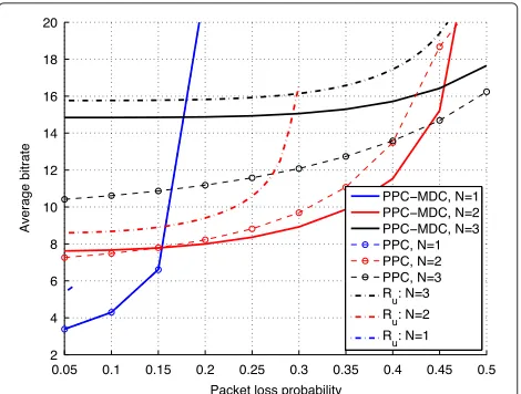
n ≈ δ2/12, which is exact for a dithered uniform quantizer and a good approximation for a non-dithered scalar uniform quantizer. We have plotted the theoretical upper bound (45) in Fig. 5 as a function of the packet loss probability and forN=1, 2, 3.
Fig. 5Average entropy. Average entropy as a function of the packet loss probability
of theMdescriptions is shown in Fig. 5 as a function of the packet loss rate andM=N.
It may be noticed in Fig. 5 that the upper bound (45) is approximately 1 bit above the estimateRT of the opera-tional bit-rates except in the region, where the packet loss rates approach and exceed the critical point, where the system becomes unstable. This excess 1 bit accounts for the theoretical loss of an entropy coder. While we have not applied actual entropy coding, it is well known that the loss of the entropy coder diminishes at moderate to large bit rates.
Note that the multiple descriptions of PPC-MDC have a certain amount of controlled redundancy, and one might therefore expect that the total coding rate for allM= N descriptions would be much greater than what is used for the single description in PPC. However, due to being a closed-loop system, packet losses affect the variance of the input to the quantizer. Consequently, the resulting coding rate for PPC as well as for PPC-MDC also depend upon the packet loss rate.
5.8 Performance
We have measured the performance of the system in terms of the average state power T1Tt=1xt22. This is shown in Fig. 6. For smaller packet loss rates, the performance of PPC is better than that of PPC-MDC forN > 1. This is because the negative impact on the performance due to quantization in PPC-MDC out-weights the impact due to using future predicted control values in PPC in case of packet losses. Recall that the quantizer in PPC-MDC is coarser than that used in PPC. When the packet loss rate is increased, PPC-MDC is often able to apply the most recent control valueu˜t(1)due to the construction of the MDs. On the other hand, PPC will frequently be applying the future predicted control valuesu˜t(2)andu˜t(3)due the
Fig. 6Average state power. Average state power as a function of the packet loss probability
packet dropouts. This leads to a significant performance gain of PPC-MDC at higher packet loss rates.
5.9 Complexity
From the analysis of the MJLS in Section 3, it is not easy to assess the computational burden required, when using the proposed system in practice. In this section, we pro-vide a brief overview of the complexity of the encoder and decoder. The encoder includes the controller, quantizer, entropy coder, and channel (FEC) coder. The decoder includes channel decoder, entropy decoder, buffering, and selection of the control values:
Encoder
1. At any given time, sayt, the control vectoru¯tis
constructed as in (10) and (13), which amount to a few matrix vector multiplications. The matrices in question are∈RN×zand ∈RN×N, whereN is the horizon length andz is the state dimension. For many applications, both the horizon length and the state dimension are moderately small.
2. Each scalar element in either the control vector
¯
ut∈RN or inξt∈RNis quantized using a scalar
quantizer as described in Section 5.6. This amounts toN simple rounding operations, which can be done efficiently in hardware.
3. The quantized elements are entropy encoded either independently, conditionally, or jointly. In either case, it is done in practice by look-up tables and is therefore of low complexity, i.e.,O(N).
thereby split the control vector intoN “layers”, then thei th layer usesi×Nmultiplications due to the
(N,i)FEC code. Thus, the total number of
multiplications isN×(1+2+ · · · +N)=O(N3).
Decoder
1. At the decoder at timet, all received packets that are no older than timet−N+1, are stored in a buffer. Moreover, all decoded control values that are no older than timet−N+1time delays are stored in another buffer. Thus, since there can beM≤N
packets in each time slot, the storage complexity is
O(MN).
2. Decoding of received packets involves decoding the FEC code and decoding the entropy code. Decoding the FEC code can be done by, e.g., Gaussian elimination, which has complexityO(N3)per layer, and therefore at mostO(N4)for decoding the entire control vector. Decoding of the entropy code is done by a look-up table and has, thus, complexityO(N), since the control vector containsN elements. 3. If the decoded control signals are stored inUt(18),
then the selection of the control signal from the buffer can be done as suggested in (19). This includes construction of the vectorδ˜iin addition to
forming the inner product ofδ˜iand the diagonal of Utindexed byγi. The inner product has complexity O(N).
6 Conclusions
We have shown how to combine multiple description cod-ing with quantized packetized predictive control, in order to get a high degree of robustness towards packet delays and erasures in network control systems. We focused on a digital network located between the controller and the plant input. In our scheme, when any single packet is received, the most recent control value becomes avail-able at the plant input. Moreover, when anyJ out ofM packets are received, the most recent control value and J−1 future predicted control values become available at the plant input. These future-predicted control values can then be applied at time instances, where no packets are received. The key motivation for this design was twofold. From a practical point of view, it was shown that a signif-icant gain over existing packetized predictive control was possible in the range of large packet loss rates. Moreover, from a theoretical point of view, computable guarantees for stability and upper bounds on the operational bit rate could be established. Indeed, a simulation study revealed that the upper bounds on the bit rate was a good indica-tor for the operational bit rate of the system in the range of packet loss probabilities that were not too close to the region of system instability.
Future works could include source coding in the feed-back channel as well as the forward channel, which is a non-trivial extension. Indeed, the design and analysis of optimal joint controller, encoders, and decoders in both forward and backward channels is an open problem even in the absence of erasures and delays. The main difficulty is that the design of the source coder in the for-ward channel hinges heavily on the design of the source coder in the backward channel as well as on the con-troller. Another interesting open research direction is to establish lower bounds on the bit rates, which will then make it possible to assess the optimality of the overall system architecture from an information theoretic point of view.
Endnotes
1For the case of quantized MPC with fixed-rate
quantization and without dithering, it was shown in [41], that the optimal quantized control vector is given by nearest neighbour quantization ofξtin (10).
2It follows that we require the dither sequence to be
known both at the encoder and at the decoder. 3We will explicitly make use of (34) – (40) and
Lemma 3.3, when assessing the stability of the system in the simulation study in Section 5.
4The excess 1 bit is due to the conservative estimate of
the loss of the entropy coder, which is characterized by 1 bit.
5If they are not of equal length, it is always possible to
augment one of the sub-bitstreams with a fixed (known) bit pattern to make them of equal length.
6Matlab code to reproduce all results (figures and
tables) will be made available online on the authors webpage.
7Of course, information about what time instances the
packets were received can be learned from past’s. How-ever, we are not exploiting this knowledge here.
Appendix 1: Proof of Lemma 3.1
Let us first consider the caseM = N. In this case, each row oftcan take onN+1 distinct patterns, i.e.,
m
!
[ 1· · ·1 N−m
!
0· · ·0] , m=0,. . .,N,
wheremdescribes the number of packets received for the time slot corresponding to that particular row. The first row oftis equivalent to the first row oft. The remain-ing rows oftcan each either be the zero vector or any one of the following:
m−k
!
[ 0· · ·0 k
!
1· · ·1 N−m
!
0· · ·0] ,m=0,. . .,N,k=1,. . .,m,
in the buffer. Thus, the number of distinct patterns for each of these rows are 1+Nm=1m. Since there is a total of N−1 of such rows, the total number of distinct difference matrices is
The case ofM<Nfollows easily from the above anal-ysis. In this case, each row oftcan only take onM+1 distinct patterns, i.e., the zero vector, or a vector con-taining the number of consecutive ones corresponding to the number of control values that are recovered, when receivingJ out of theMpackets, whereJ = 1,. . .,M. It follows immediately that the number of possible differ-ence indicator matrices is less forM < N compared to M=N.
Appendix 2: Proof of Lemma 3.2
We first prove ergodicity. Clearly, from the all zero dif-ference indicator matrix, it is possible to get to any other difference indicator matrix in a finite number of steps. Moreover, the probability of not receiving any packets in N consecutive time steps is positively bounded away from zero for any finiteN. The all zero difference indica-tor matrix can therefore be reached in a finite number of steps (from any other difference indicator matrix). Thus, it is possible to jump between any two difference indica-tor matrices in a finite number of steps. We may therefore view the difference indicator matrices as being the differ-ent nodes in a fully connected graph. In this graph, any node can be reached at irregular times. Thus, the nodes are recurrent and aperiodic, which implies that they are are ergodic and the sequence{t}of difference indicator matrices is therefore also ergodic.
We now prove the Markovian property. Observe that the matrices in the sequence{t}are not mutually inde-pendent. However, the sequence does satisfy a first-order Markov condition due to the Markov assumption on the data reception, see Section 2.3, i.e.,
t−1
0 ↔t↔t+1, ∀t, (48)
which implies that knowledge of the bufferf¯t−1does not bring moreuseful7information about the buffer¯ft+1if the bufferf¯tis already known. Similarly, it is easy to see that the sequence{t}of difference matrices form a Markov chain similar to (48), i.e.,
{
i}ti=−01↔t ↔t+1, ∀t. (49)
Finally, the stationarity of the channel, see Section 2.3, implies that the sequence of difference matrices{t} is
stationary. This proves the lemma.
Appendix 3: Proof of Theorem 3.1
In Lemma 3.2, we have established ergodicity and Markov properties of the switching sequence{t}as is required by Lemma 3.3. We then need to derive the recursive form for the system evolution, which guarantees that the combined system{t,t}will be Markovian.
Recall from (19) that¯ft(i) = ˜δiTγi(Ut)fori= 1,. . .,N. However, to avoid updating the buffer with information about packets that was already received in previous time instances, we need to look only at the changes betweent andt−1. Towards that end, letδi γi(t−S↓t−1). Defineδ˜iin a similar manner asδ˜i. Ifδiis the all zero vec-tor for somei, it means that no new control signals to be used at time t+i−1 has been received yet. Thus, the ith element of the buffer is then simply obtained by using older control signals, i.e.,¯ft(i)= ¯ft−1(i+1). With this, we
With the above notation, the system state vector recur-sions can be written as:
xt+1=Axt+B1(δ˜1Tγ1(Ut)
and combining (51) and (50) and
using the matrix definitions in (24) – (33) yields (23). This
proves the theorem.
Appendix 4: Proof of Theorem 3.3
In order to provide an upper bound on the required bit rate for transmitting the quantized control vectorξt, we assume that the system is designed such that the loop is AWSS. For such a system, the bit rateRof the ECDQ is related to the discrete entropyH(ξt|ζt)of the quantized signalξt, conditioned upon the dither signalζt[31]. That is,
H(ξt|ζt)≤R≤H(ξt|ζt)+1/N, (52)
sendξtusingMdescriptions such that upon receiving any 0<J≤Mdescriptions, theJcontrol signalsu˜t(1),. . .,u˜t can be reliably recovered. This is clearly not possible ifξt is arbitrarily split intoM sub-streams having a total bit rate ofH(ξt|ζt). In Section 4.2, we introduced a practical scheme for MDs based on forward error correction codes. With this scheme, a description is constructed by con-catenating the entire bitstream used for representing the encoded version ofu˜t(1)with half the bitstream used for
˜
ut(2), one third of the bits allocated foru˜t(3), and so on. With such a scheme in mind, we first invoke the chain rule of entropies, in order to expandH(ξt|ζt)in (52) as:
H(ξt|ζt)=H(ξt(1)|ζt)+H(ξt(2)|ξt(1),ζt)+ · · · +H(ξt(N)|ξt(1),. . .,ξt(N−1),ζt). (53)
The ith term on the r.h.s. of (53), describes the min-imum bit rate required for conditionally encoding ξt(i). With this, and using the MD construction sketched above, the total rateRT required for allM = Ndescriptions is given by:
RT ≤M
H(ξt(1)|ζt)+ 1 2H(ξ
t(2)|ξt(1),ζt)+ · · ·
+ 1
MH(ξ
t(N)|ξt(1),. . .,ξt(N−1),ζt)
+1. (54)
Since we are using an ECDQ, the discrete entropy of the quantized variables satisfies:
H(ξt|ζt)=I(ξt;ξˆt) (55)
=I(ξt;ξt+nt) (56)
≤I(ξ¯t;ξ¯t+ ¯nt)+D(nt¯nt), (57)
where equality in (55) follows from [31] and whereI(ξt;ξˆt) denotes the mutual information [30] between the inputξt and the outputξˆt of the ECDQ [31]. In (56), the equal-ity follows by replacing the quantization operation by its additive noise model, which is exact from a statistical point of view [31]. The upper bound in (57) follows from ([43] Lemma 2) by replacing the variables in play by their Gaussian counterparts, i.e.,ξ¯t and n¯t are Gaussian dis-tributed with the same first- and second moments asξt and nt, respectively. The Divergence operator D(nt¯nt) describes the Kullback-Leibler distance (in bits) between the distribution of the quantization noise nt to that of a Gaussian distribution [30] and is in our case upper bounded by D(nt¯nt) ≤ N/2 log2(πe/6). This upper bound is achieved if nt is uniformly distributed over
an N-dimensional cube [44]. We may now proceed by
expressing the mutual information in terms of differential entropies provided the latter exists [30]. Thus, we obtain thatI(ξ¯t;ξ¯t+ ¯nt) = h(ξ¯t + ¯nt)−h(n¯t). Using the same idea on the conditional estimatesξt(i)|ξt(1),· · ·,ξt(i−1) instead of the entire vectorξtleads to:
H(ξt(i)|ξt(1),. . .,ξt(i−1),ζt)
≤h(ξ¯t(i)|¯ξt(1),· · ·,ξ¯t(i−1)+ ¯nt(i))−h(n¯t(i)) +1/2 log2(πe/6)
= 1
2log2
1+ σ 2
ξ(i)|ξ(1),···,ξ(i−1) σ2
n
+1
2log2
πe
6
,
(58)
where the last equality follows from the definition of dif-ferential entropy of a Gaussian variable [30]. Inserting (58) into (54) and (52) yields (45). This completes the proof.
Competing interests
The authors declare that they have no competing interests.
Acknowledgements
This research was partially supported by VILLUM FONDEN Young Investigator Programme, Project No. 10095. The authors would like to thank the reviewers for pointing us to references [23–25] and to [6, 7].
Author details
1Department of Electronic Systems, Aalborg University, Fredrik Bajers Vej 7b,
Aalborg, Denmark.2Department of Electrical Engineering (EIM-E), Paderborn University, Paderborn, Germany.
Received: 21 October 2015 Accepted: 28 March 2016
References
1. JP Hespanha, P Naghshtabrizi, Y Xu, A survey of recent results in networked control systems. Proc. IEEE.1(95), 138–162 (2007) 2. GN Nair, F Fagnani, S Zampieri, RJ Evans, Feedback control under data
rate constraints: an overview. Proc. IEEE.95(1), 108–137 (2007) 3. S Wong, RW Brockett, Systems with finite communication band- width
constraints ii: stabilization with limited information feedback. IEEE Trans. Autom. Control.44(5), 1049–1053 (1999)
4. M Trivellato, N Benvenuto, State control in networked control systems under packet drops and limited transmission bandwidth. IEEE Trans. Commun.58(2), 611–622 (2010)
5. DE Quevedo, A Ahlén, J Østergaard, Energy efficient state estimation with wireless sensors through the use of predictive power control and coding. IEEE Trans. Signal Process.58(9), 4811–4823 (2010)
6. T Wang, Y Zhang, J Qiu, H Gao, Adaptive fuzzy backstepping control for a class of nonlinear systems with sampled and delayed measurements. IEEE Trans. Fuzzy Syst.23(2), 302–312 (2015)
7. T Wang, H Gao, J Qiu, A combined adaptive neural network and nonlinear model predictive control for multirate networked industrial process control. IEEE Trans. Neural Netw. Learn. Syst.27(2), 416–425 (2016) 8. PL Tang, CW de Silva, Compensation for transmission delays in an
Ethernet-based control network using variable-horizon predictive control. IEEE Trans. Contr. Syst. Technol.14(4), 707–718 (2006)
9. G Liu, Y Xia, J Chen, D Rees, W Hu, Networked predictive control of systems with random network delays in both forward and feedback channels. IEEE Trans. Ind. Electron.54(3), 1282–1297 (2007) 10. DE Quevedo, D Neši´c, Input-to-state stability of packetized predictive
control over unreliable networks affected by packet-dropouts. IEEE Trans. Autom. Control.56(2), 370–375 (2011)
11. DE Quevedo, J Østergaard, Nesi´c, Packetized predictive control of stochastic systems over digital channels with random packet loss. IEEE Trans. Autom. Control.56(12), 2854–2868 (2011)
12. AAE Gamal, TM Cover, Achievable rates for multiple descriptions. IEEE Trans. Inf. Theory.IT-28(6), 851–857 (1982)
13. VK Goyal, Multiple description coding: compression meets the network. IEEE Signal Proc. Mag.18(5), 74–93 (2001)


![Fig. 4 Spectral radius. Spectral radiusand as a function of the packet loss probability σr(A) of A in (34) for N = 1, 2, 3 p ∈ [ 0, 0.5]](https://thumb-us.123doks.com/thumbv2/123dok_us/886089.1106495/11.595.307.542.87.262/fig-spectral-radius-spectral-radiusand-function-packet-probability.webp)