ABSTRACT
ZHANG, XIANG. Contributions to Statistical Methods for High Dimensional and Dependent Data. (Under the direction of Alyson Wilson and Lexin Li.)
In this thesis, we develop three new statistical methods for high dimensional and dependent data. The three methods are motivated by three independent projects.
In the first project, we investigate variable selection for support vector machines for high dimensional data. A general class of non-convex penalized support vector machines is proposed. We show that one of the local solutions to the non-convex penalized support vector machines is the oracle estimator. This is the first variable selection consistency result for support vector machines in high dimensions. We also present an algorithm with provable global convergence to the oracle estimator. Our proof techniques are novel and do not require the differentiability of the loss function, which extend the existing results in the literature where the loss function is restricted to be a smooth function.
In the second project, we study system reliability and component importance for dependent systems. We establish a unified and general framework to characterize the influence of a de-pendence structure on system reliability and component importance. Our results are based on recent developments for copula theory with discrete marginal distributions. We reveal the con-nections of system reliability and component importance under dependence to some well-known principles under independence assumption. We also extend our results to multi-state system. Our derived results are further demonstrated using a Gaussian copula, and we show that the effects of dependence under a Gaussian copula have simple interpretations.
©Copyright 2016 by Xiang Zhang
Contributions to Statistical Methods for High Dimensional and Dependent Data
by Xiang Zhang
A dissertation submitted to the Graduate Faculty of North Carolina State University
in partial fulfillment of the requirements for the Degree of
Doctor of Philosophy
Statistics
Raleigh, North Carolina 2016
APPROVED BY:
Alyson Wilson
Co-chair of Advisory Committee
Lexin Li
Co-chair of Advisory Committee
Yichao Wu Ralph Smith
DEDICATION
BIOGRAPHY
ACKNOWLEDGEMENTS
My five years at North Carolina State University has been one of the most pleasant times in my life. I want to thank all of the people who have made this happen.
I want to thank my advisor Alyson Wilson for her constant support and help for my re-search in reliability modeling. From her I learned to start the problem with simple ideas and keep building up step by step. She is patient when I make mistakes, and her words are al-ways encouraging. I am not only grateful for her funding to support my research, but also her continuous guidance that has to lead to this thesis.
I owe my special thanks to my co-advisor Lexin Li for leading me into the world of imaging and network data. He is always willing to walk through the details with me, and his insights have reshaped my understandings of many statistical problems. The time we spent reading through the literature together is one of the most enjoyable times I had in my research.
I want to thank Yichao Wu for opening the door of the first research project in my life for me. Without his faith in me I couldn’t have made it this far.
I owe my thanks to Ralph Smith and Gregory Hicks for serving on my committee. Their feedback is important to my research. I also want to thank Hua Zhou and Arnab Maity for their helpful questions and comments during my oral exam.
The Department of Statistics is a great place. I want to thank Donald Martin, Howard Bondell, Eric Laber, and Eric Chi for their helpful advice in my study. I also want to thank all the department staff for always being there to make thinks work.
I learned many things from my fellow students. I owe Yichi Zhang for answering so many questions for me when I was stuck. I want to thank especially Weining Shen for all the invaluable advice about my PhD studies. I want to thank Shikai Luo, Zhou Li, Zhongkai Liu, Ailin Fan, Yan Zhang, Hao Hu, and Teng Zhang for making the study at here a nice thing throughout the years.
in my life. I am grateful for Damon Amato, Richard Forth, Ted Davis, Mark Ferguson, Anil Samuel, Jonathan Peck, Leslie Ratliff, Dan Crompton, Lijoy Samuel and Abdallah Shammas, for showing their love and shedding the light in my life.
Much credit goes to my parents. They may know nothing about my research projects, but they have contributed the most to this thesis. Without their support for me to study abroad, nothing could have been achieved.
TABLE OF CONTENTS
LIST OF TABLES . . . .viii
LIST OF FIGURES . . . ix
Chapter 1 Introduction . . . 1
1.1 High Dimensional and Dependent Data Overview . . . 1
1.2 Motivating Examples . . . 2
1.3 Plan of Dissertation . . . 4
Chapter 2 Variable Selection for Support Vector Machines . . . 6
2.1 Introduction . . . 6
2.2 Methodology . . . 8
2.3 Theory . . . 10
2.3.1 Regularity Conditions . . . 10
2.3.2 Oracle Property . . . 12
2.3.3 An Algorithm with Provable Convergence to the Oracle Estimator . . . . 16
2.4 Simulations . . . 19
2.5 Real Data . . . 24
2.6 Proofs . . . 25
Chapter 3 Reliability Modeling for Dependent Systems . . . 37
3.1 Introduction . . . 37
3.2 Main Results . . . 40
3.2.1 System Reliability with Dependence . . . 41
3.2.2 Component Importance with Dependence . . . 47
3.2.3 Extensions to Multi-State Systems . . . 51
3.3 Implementation . . . 53
3.4 Simulations . . . 55
3.4.1 System Reliability with Dependence . . . 55
3.4.2 Component Importance with Dependence . . . 59
3.5 Real Data . . . 61
3.6 Proofs . . . 69
Chapter 4 Longitudinal Tensor Regression . . . 75
4.1 Introduction . . . 75
4.2 Methodology . . . 77
4.3 Implementation . . . 80
4.4 Theory . . . 82
4.4.1 Regularity Conditions . . . 82
4.4.2 Consistency and Asymptotic Normality . . . 83
4.4.3 Rank Selection Consistency . . . 85
4.5 Simulations . . . 87
4.6 Real Data . . . 93
4.7 Proofs . . . 95
Chapter 5 Discussion . . . .113
5.1 Contributions . . . 113
5.2 Future Work . . . 114
LIST OF TABLES
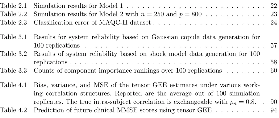
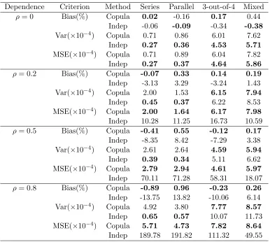
Table 2.1 Simulation results for Model 1 . . . 22 Table 2.2 Simulation results for Model 2 with n= 250 andp= 800 . . . 23 Table 2.3 Classification error of MAQC-II dataset . . . 24 Table 3.1 Results for system reliability based on Gaussian copula data generation for
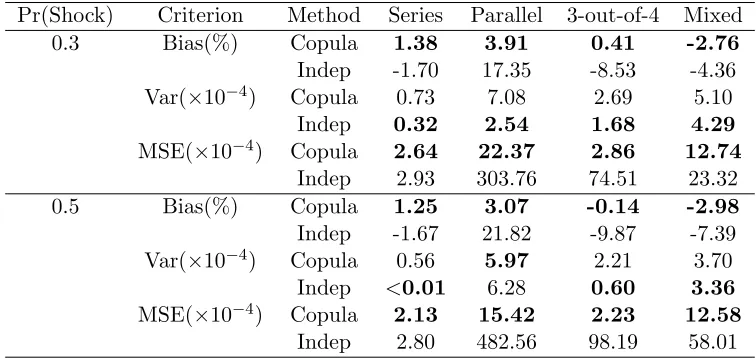
100 replications . . . 57 Table 3.2 Results of system reliability based on shock model data generation for 100
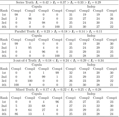
replications . . . 58 Table 3.3 Counts of component importance rankings over 100 replications . . . 60 Table 4.1 Bias, variance, and MSE of the tensor GEE estimates under various
LIST OF FIGURES
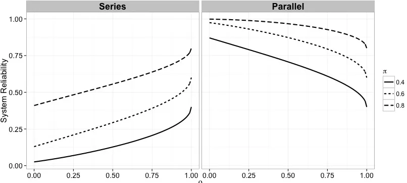
Figure 3.1 For fixedπ, the series system reliability increases withρ, while parallel system reliability decreases withρ. . . 47 Figure 3.2 Posterior densities of π from the first data set with dropped-missing data.
The copula model and independence model give almost identical marginals estimations, which agree with the MLE’s (vertical lines). . . 63 Figure 3.3 Posterior densities ofΣ= (ρij) from the first data set with dropped-missing
data. The positive associations are captured byρ >0. . . 63 Figure 3.4 Posterior distributions ofΣ= (ρij) from the first data set with the fill-missing
data. . . 64 Figure 3.5 Posterior densities of system reliability from the first data set. The vertical
line shows the true system reliability from system-level data. For either the dropped-missing data (n=57) or fill-missing data (n=169), the copula model fits the system-level data better. . . 65 Figure 3.6 Posterior predictive distributions of system passes from the first data set.
For either the dropped-missing data (n=57) or fill-missing data (n=169), the predictive distribution from copula model is closer to the observed number of system passes (dashed lines). . . 65 Figure 3.7 Posterior distributions of component importance from the first data set with
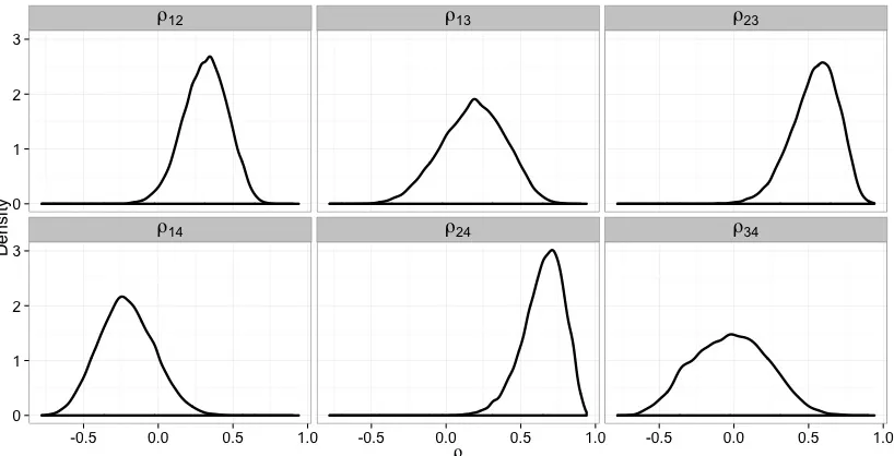
dropped-missing data. The ranking of component reliability importance takes into account the dependence structure under the copula model. . . 66 Figure 3.8 Posterior distributions of Σ = (ρij) from the second data set with the
fill-missing data. It can be seen thatρ14and ρ34 have large posterior probabili-ties of being negative, suggesting the positive association assumption among components fails. . . 67 Figure 3.9 Posterior predictive distributions of system passes from the second data set
using the fill-missing data. The dashed lines show the observed number of system passes. The copula model fits the observed system-level data better than the independence model. . . 68 Figure 4.1 True and recovered image signals by the tensor GEE with varying ranks.
n = 500, m = 4. The correlation structure is correctly specified. TR(R) means estimate from the rank-R tensor model. . . 89 Figure 4.2 Snapshots of tensor GEE estimation with different working correlation
Chapter 1
Introduction
1.1
High Dimensional and Dependent Data Overview
The central theme of this thesis is the development of new statistical methods for certain high dimensional and dependent data problems. The proposed methods in this thesis can be viewed as extensions of some traditional statistical approaches to specifically meet the challenges from high dimensional and dependent data. We first present an overview of the data that are considered as high dimensional and dependent in this thesis.
By high dimensional, we mean that the number of predictors, or variables, is large, while the number of instances, or samples, is only moderate. As a result, the number of predictors is much larger than the number of instances. The direct challenge of high dimensional data is that we do not have enough information in the data to estimate a full model constructed using all the available predictors. The estimated model without variable selection would be either ill-conditioned or subject to severe overfitting. Another challenge is that a model directly built from high dimensional data is complex and difficult to interpret in general, which limits its applications in practice.
However, there are some scenarios when the independence assumption may not be realistic. A naive model that simply ignores the dependency within the data is essentially allowing model misspecification, which can result in considerable biases in the estimators.
In Section 1.2, we introduce three real-world examples. The first is an example of high dimensional data, the second is an example of dependent data, and the third is an example that contains both high dimensional and dependent data simultaneously. These three examples motivate the proposed statistical methods discussed in later chapters of this thesis.
1.2
Motivating Examples
1. MAQC-II Data
This data is part of the MicroArray Quality Control (MAQC)-II project. The complete data is available at the GEO database with accession number GSE20194 athttp://www. ncbi.nlm.nih.gov/geo/query/acc.cgi?acc=GSE20194. It contains 278 patient samples. Each sample is described by the expression values of 22,283 genes. For each sample, the estrogen receptor (ER) status, positive or negative, is also available. The goal of the analysis is to build a binary classifier to predict the ER status from the information contained in the genes. For the 278 patient samples, 164 patients have positive ER status and 114 patients have negative ER status.
This is an example of high dimensional data. The number of genes is much larger than the number of instances in this data. To predict the ER status, one can consider building a classifier using all of the genes. However, given the small sample size, the full model is likely to be overfitted and thus making noisy predictions. The challenge of this data is to select a small subset of genes from all the available variables and build the classifier only using those selected genes.
2. Stockpile Test Data
of simple military systems. The two data sets represent different variants of a system with slightly different functionality. Test results on components and the full system are available. For both data, the system is constructed to be a series system, and a pass for the overall system means that all of the components performed as required. We are interested in the estimating the system reliability and identifying the most critical component to the system. The first data set consists of 169 tests on a four-component system. The second data set consists of 181 tests on a four-component system.
This is an example of dependent data. The test results of components within a system are likely to be dependent in practice. There are several possible sources of the dependence among components. The components may be subject to some common stress so that they are more likely to function or fail at the same time. The components may share loads in the system so that if one component fails, the remaining components have to share more loads and thus are more likely to fail as well. In Chapter 3, we provide more evidence to show that the independence assumption is unlikely to hold for the stockpile test data. The challenge of this data is to take into account the dependence among components in modeling the system reliability and component importance.
3. Longitudinal Imaging Data
useful for monitoring disease progression.
This is an example of both high dimensional and dependent data. If all the pixels in the MRI image are used as predictors, the total number of predictors is 323= 32,768, which is much larger than the available sample size 88×5 = 440. Therefore, this data is high dimensional by our definitions. This data is also longitudinal, meaning that there are repeated measures of the same subject across different time points. In this example, the MMSE scores of the same subject across five time points are dependent. Two challenges arise in the analysis of this data. The first challenge of this data is to find a parsimonious model for the high dimensional image covariates. Another challenge is to capture the temporal dependence in the data.
1.3
Plan of Dissertation
This thesis consists of three projects, motivated by the data examples in Section 1.2. The first project provides a new statistical approach to address the high dimensionality in the MAQC-II data. This project is presented in Chapter 2. The second project proposes a copula approach to capture the dependence in the stockpile test data. This project is discussed in detail in Chapter 3. The third project presents a new method to analyze high dimensional and dependent longitudinal imaging data. We investigate this method in depth in Chapter 4. Summary of the contributions and extensions of the three projects are discussed in Chapter 5.
1. First Project (Chapter 2)
2. Second Project (Chapter 3)
This project is motivated by the stockpile test data. We characterize the influence of dependence structures on system reliability and component importance in coherent sys-tems with discrete marginal distributions. The main tool we use is copula theory. We also extend our results to more general coherent multi-state system. We demonstrate the applications of our derived results using Gaussian copulas, which yield simple interpreta-tions. We conduct simulations and analyze two real-world examples based on the stockpile test data to demonstrate the advantages of the copula model over a naive independence model in estimating system reliability and component importance.
3. Third Project (Chapter 4)
Chapter 2
Variable Selection for Support
Vector Machines
This chapter is organized as follows. Section 2.1 gives the introduction and the setup of the problem. In Section 2.2, we introduce the proposed method. Section 2.3 contains the theoretical studies, followed by simulation studies in Section 2.4 and results on real world MAQC-II data in Section 2.5. The technical proofs are presented in Section 2.6.
2.1
Introduction
We consider the Support Vector Machine (SVM, Vapnik, 1996) for the MAQC-II data. SVM is a powerful binary classification tool with high accuracy and great flexibility. It has achieved success in many applications. In binary classification, we are typically given a random sample
ifYi =−1 for some 0< w <1, the linear weighted support vector machine (WSVM, Lin et al., 2002) estimates the classification boundary by solving
min
β n
−1 n
X
i=1
Wi(1−YiXiTβ)++λ(β∗)Tβ∗,
where (1−u)+= max{1−u,0}denotes the hinge loss,λ >0 is a regularization parameter, and β= (β0,(β∗)T)Twithβ∗= (β1, β2,· · · , βp)T. The standard SVM is a special case of the WSVM with weight parameterw= 0.5. In this thesis, we consider the WSVM for more generality.
One drawback of the standard SVM is that its performance can be adversely affected if many redundant variables are included in building the decision rule (Friedman et al., 2001). In general, the corresponding decision rule, sign(XTβ), uses all covariates and is not capable
of selecting relevant covariates. Classification using all features has been shown to be as poor as random guessing due to noise accumulation in high dimensional space (Fan and Fan, 2008). For the MAQC-II data, it is known that the only a subset of genes are informative to the ER status. Simply using all the available genes without variable selection does not give the optimal prediction accuracy, see the evidence in Section 2.5.
Many methods have been proposed to remedy this problem, such as the recursive fea-ture elimination suggested by Guyon et al. (2002). In particular, superior performance can be achieved with a unified method, namely achieving variable selection and prediction simultane-ously (Fan and Li, 2001) by using an appropriate sparsity penalty. It is well known that the standard SVM can fit in the regularization framework of loss+penalty using the hinge loss and L2 penalty. Based on this, several attempts have been made to achieve variable selection for the SVM by replacing theL2penalty with other forms of penalty. Bradley and Mangasarian (1998), Zhu et al. (2004), and Wegkamp and Yuan (2011) considered the L1-penalized SVM; Zou and Yuan (2008) proposed to use the F∞-norm SVM to select groups of predictors; Wang
et al. (2011) and Park et al. (2012) studied the smoothly clipped absolute deviation (SCAD, Fan and Li, 2001)-penalized SVM. Recently Park et al. (2012) studied the oracle property of the SCAD-penalized SVM with a fixed number of predictors. Yet, to the best of our knowledge, the theory of variable selection consistency of sparse SVMs in high dimensions or ultra-high dimensions (Fan and Lv, 2008) has not been studied so far.
2.2
Methodology
In this section we propose a general class of non-convex penalized SVMs that can achieve variable selection and prediction simultaneously. As we will show, our proposed method is the first one that possesses variable selection consistency in high dimensions.
We begin with the basic setup and notation. Consider the population linear weighted hinge lossE{W(1−YXTβ)+}. Letβ0 = (β00, β01, . . . , β0p)T= (β00,(β0∗)T)Tdenote the true parameter value, which is defined as the minimizer of the population weighted hinge loss. Namely
β0= arg min
β E{W(1−YX
T
β)+}. (2.1)
The number of covariates p = pn is allowed to increase with the sample size n. It is even possible that pn is much larger than n. In this project we assume the true parameter β0 to be sparse. Let A = {1 ≤ j ≤ pn;β0j 6= 0} be the index set of the nonzero coefficients. Let
q=qn=|A|be the cardinality of set A, which is also allowed to increase withn. Without loss of generality, we assume that the lastpn−qncomponents ofβ0are zero. That is,βT0 = (βT01,0T). Correspondingly, we write XT
i = (ZiT,RTi), where Zi = (Xi0, Xi1, . . . , Xiq)T = (1,(Zi∗)T)T and Ri = (Xi[q+1], . . . , Xip)T. Further we denoteπ+(resp.π−) to be the marginal probability of the
label Y = +1 (resp. -1).
We propose the non-convex penalized hinge loss objective function:
Q(β) =n−1
n
X
i=1
Wi(1−YiXT
iβ)++ pn X
j=1
where pλn(·) is a symmetric penalty function with tuning parameter λn. Let p
0
λn(t) be the
derivative of pλn(t) with respect tot. We consider a general class of non-convex penalties that
satisfy the following conditions.
(Condition 1) The symmetric penalty pλn(t) is assumed to be nondecreasing and concave
fort∈[0,+∞), with a continuous derivativep0λn(t) on (0,+∞) and pλn(0) = 0.
(Condition 2) There exists a > 1 such that limt→0+p0λn(t) = λn, p0λn(t) ≥ λn−t/a for 0< t < aλand p0λ
n(t) = 0 fort≥aλ.
The motivation for such a non-convex penalty is that the convexL1 penalty lacks the oracle property due to the overpenalization of large coefficients in the selected model. Consequently it is undesirable to use the L1 penalty when the purpose of the data analysis is to select the relevant covariates among potentially high dimensional candidates in classification. Note that
p,q,λand other related quantities are allowed to depend on n, and we suppress the subscript
nwhenever there is no confusion.
Two commonly used non-convex penalties that satisfy Conditions 1 and 2 are the SCAD and MCP penalties. The SCAD penalty (Fan and Li, 2001) is defined by
pλ(|β|) =λ|β|I(0≤ |β|< λ) +
aλ|β| −(β2+λ2)/2
a−1 I(λ≤ |β| ≤aλ) +
(a+ 1)λ2
2 I(|β|> aλ)
for somea >2. The MCP (Zhang, 2010) is defined by
pλ(|β|) =λ(|β| −
β2
2aλ)I(0≤ |β|< aλ) + aλ2
2 I(|β| ≥aλ) for some a >1.
By acting as if the true sparsity structure is known in advance, the oracle estimator is defined asβb= (βbT1,0T)T, where
b
β1= arg min
β1 n−1
n
X
i=1
Wi(1−YiZT
iβ1)+. (2.3)
proposed method can find an estimator converge to the desirable oracle estimator with high probability.
2.3
Theory
2.3.1 Regularity Conditions
To facilitate our theoretical analysis, we introduce the gradient vector and Hessian matrix of the population linear weighted hinge loss. LetL(β1) =E{W(1−YZTβ1)+}be the population
linear weighted hinge loss using only relevant covariates. Define S(β1) = (S(β1)j) to be the (qn+ 1)-dimension vector given by
S(β1) =−E{I(1−YZT
β1≥0)W YZ},
whereI(·) denotes the indicator function. Also defineH(β1) = (H(β1)jk) to be the (qn+ 1)× (qn+ 1) matrix given by
H(β1) =E{δ(1−YZTβ1)WZZT},
where δ(·) denotes the Dirac delta function. It can be shown that if well-defined, S(β1) and
H(β1) can be considered to be the gradient vector and Hessian matrix of L(β1), respectively. See Lemma 2 of Koo et al. (2008) for details.
We impose the following regularity conditions:
(A1) The densities of Z∗ given Y = +1 and Y = −1 are continuous and have common support in Rq.
(A2) E[Xj2]<∞ for 1≤j≤q.
(A3) The true parameter β0 is unique and a nonzero vector.
(A4) qn=O(nc1), namely limn→∞qn/nc1 <∞, for some 0≤c1 <1/2.
assumed that max1≤i≤n||Zi||=Op(
√
qnlog(n)), (Zi, Yi) are in general position (Koenker, 2005, sect. 2.2), Xij are sub-Gaussian random variables for 1≤i≤n, qn+ 1≤j≤pn.
(A6) λmin(H(β01)) ≥ M2 for some constant M2 > 0, where λmin denotes the smallest eigenvalue.
(A7) n(1−c2)/2min1
≤j≤qn|β0j| ≥M3 for some constantM3 >0 and 2c1 < c2 ≤1.
(A8) Denote the conditional density of ZTβ01 given Y = +1 and Y = −1 as f and g,
respectively. It is assumed thatf is uniformly bounded away from 0 and ∞in a neighborhood of 1 andg is uniformly bounded away from 0 and ∞ in a neighborhood of -1.
Conditions (A1)-(A3) and (A6) are also assumed for fixed p in Koo et al. (2008). We need these assumptions to ensure that the oracle estimator is consistent in the scenario of diverging
p. Condition (A3) states that the optimal classification decision function is not constant, which is required to ensureS(β) andH(β) are well-defined gradient vector and Hessian matrix of the hinge loss, see Lemma 2 and Lemma 3 of Koo et al. (2008). The conditions (A4) and (A7) are common in the literature on high dimensional inference (Kim et al., 2008). More specifically, (A4) states that the divergence rate of the number of nonzero coefficients cannot be faster than root-nand (A7) simply states that the signals cannot decay too quickly. The condition on the largest eigenvalues of the design matrix in (A5) is similar to the sparse Riesz condition and also assumed in Zhang and Huang (2008), Yuan (2010) and Zhang (2010). Note that the bound on the smallest eigenvalue is not specified. The condition on the maximum norm in (A5) holds when Z∗ given Y follows multivariate normal distribution. (Zi, Yi) are in general position if with probability one there are exactly (qn+ 1) elements inD={i: 1−YiZiTβ1b = 0} (Koenker,
2005, sect. 2.2). The condition for general position is true with probability one w.r.t. Lebesgue measure. Condition (A8) requires that there is enough information around the nondifferentiable point of the hinge loss, similar to condition (C5) in Wang et al. (2012) for quantile regression. For illustrative examples that satisfy all the above conditions, assume 0< π+= 1−π− <1
Fisher’s discriminant analysis is one special case when X∗ given Y are Gaussian. Conditions (A1)-(A4) and (A7) are trivial. Condition (A5) holds by the properties of sub-Gaussian random variable. Koo et al. (2008) showed that Condition (A6) holds if the supports of the conditional densities of Z∗ given Y are convex, which are naturally satisfied for Rq. Condition (A8) is
trivially satisfied by the unbounded support of the conditional distribution ofZ∗ given Y. Another example is the Probit model thatX∗has unbounded supportRpwith sub-Gaussian
tails and Pr(Y = +1|X∗) = Φ(XTβ) for some β 6= 0. It can be easily checked that the
conditional distributions of X∗ given Y also have unbounded supports Rp and hence all the
conditions are satisfied.
2.3.2 Oracle Property
In this subsection, we establish the theory of the oracle property for non-convex penalized SVMs; namely, the oracle estimator is one of the local minimizers of the objective function
Q(β) defined in (2.2). We start with the following lemma on the consistency of the oracle estimator, which can be viewed as an extension of the consistency result in Koo et al. (2008) to the divergingp scenario.
Lemma 2.1. Assume that Conditions (A1)-(A7) are satisfied. The oracle estimator βb =
(βb1T,0T)T satisfies ||βb1−β01||=Op( p
qn/n) when n→ ∞.
Though the convexity of the non-convex penalized hinge loss objective function Q(β) is not guaranteed, it can be written as the difference of two convex functions:
Q(β) =g(β)−h(β), (2.4)
whereg(β) =n−1Pn
i=1Wi(1−YiXiTβ)++λnPpj=1|βj|andh(β) =λnPpj=1|βj|−Ppj=1pλn(|βj|) = Pp
we have
Hλ(βj) = [(βj2−2λ|βj|+λ2|)/{2(a−1)}]I(λ≤ |βj| ≤aλ) +{λ|βj| −(a+ 1)λ2/2}I(|βj|> aλ),
while for MCP, we haveHλ(βj) ={βj2/(2a)}I(0≤ |βj|< aλ)+(λ|βj|−aλ2/2)I(|βj| ≥aλ). This decomposition is useful, as it naturally satisfies the form of the difference of convex functions (DC) algorithm (An and Tao, 2005).
To prove the oracle property of the non-convex penalized SVMs, we will use a sufficient local optimality condition for the difference convex programming first presented in Tao and An (1997). This sufficient condition is based on subgradient calculus. The subgradient can be viewed as an extension of the gradient of the smooth convex function to the non-smooth convex function. Let dom(g)={x : g(x) < ∞} be the effective domain of a convex function g. The subgradient of g(x) at a point x0 is defined as ∂g(x0) = {t : g(x) ≥ g(x0) + (x−x0)Tt}. Note that at the non-differentiable point, the subgradient contains a collection of vectors. One can easily check that the subgradient of the hinge loss function at the oracle estimator is the collection of vectorss(β) = (b s0(β)b , . . . , sp(β))b T with
sj(β) =b −n−1
n
X
i=1
WiYiXijI(1−YiXiTβb>0)−n−1
n
X
i=1
WiYiXijvi, (2.5)
where−1≤vi ≤0 if 1−YiXiTβb= 0 and vi = 0 otherwise,j= 0, . . . , p. Under some regularity
conditions, we can study the asymptotic behaviors of the subgradient at the oracle estimator. The results are summarized in the following Theorem.
with vi =vi∗, with probability approaching one, we have
sj(β) = 0b , j= 0,1, . . . , q, |βˆj| ≥(a+
1
2)λ, j = 1, . . . , q,
|sj(β)b | ≤λ, j =q+ 1, . . . , p, |βˆj|= 0, j =q+ 1, . . . , p.
Theorem 2.1 characterizes the subgradients of the hinge loss at the oracle estimator. It basically says that in a regular setting, with probability arbitrarily close to one, those compo-nents of the subgradients corresponding to the relevant covariates are exactly zero and those corresponding to irrelevant covariates are not far away zero.
We now present the sufficient optimality condition based on subgradient calculations. Corol-lary 1 of Tao and An (1997) states that if there exists a neighborhoodU around the point x∗ such that ∂h(x)∩∂g(x∗) 6=∅,∀x∈U ∩dom(g), then x∗ is a local minimizer ofg(x)−h(x). To verify this local sufficient condition, we study the asymptotic behaviors of subgradients of the two convex functions in the aforementioned decomposition (2.4) ofQ(β). Note that, based on (2.5), the subgradient function ofg(β) atβ can be shown to be the following collection of vectors:
∂g(β) =nξ= (ξ0, . . . , ξp)T∈ Rp+1 :
ξj =−n−1 n
X
i=1
WiYiXijI(1−YiXiTβb>0)−n−1
n
X
i=1
WiYiXijvi+λlj, j= 0, . . . , p
o ,
where l0 = 0, lj = sgn(βj) ifβj 6= 0 and lj ∈[−1,1] otherwise for 1≤j ≤p, and−1≤vi ≤0 if 1−YiXiTβb = 0 and vi = 0 otherwise for 1 ≤ i ≤ n. Furthermore, by Condition 2 of the
class of non-convex penalty functions, limt→0+Hλ0(t) = limt→0−Hλ0(t) =λsgn(t)−λsgn(t) = 0.
singleton:
∂h(β) ={µ= (µ0, . . . , µp)∈ Rp+1 :µj =
∂h(β)
∂βj
, j = 0, . . . , p}.
For the class of non-convex penalty functions under consideration, ∂h(∂ββ)
j = 0 for j = 0. For
1≤j≤p,
∂h(β)
∂βj
= [{βj−λsgn(βj)}/(a−1)]I(λ≤ |βj| ≤aλ) +λsgn(βj)I(|βj|> aλ)
for the SCAD penalty, and
∂h(β)
∂βj
= (βj/a)I(0≤ |βj|< aλ) +λsgn(βj)I(|βj| ≥aλ)
for the MCP.
Combining this with Theorem 2.1, we will prove that with probability tending to one, for any βin a ball inRp+1with the centerβband radius λ2, there exists a subgradientξ= (ξ0, . . . , ξp)T∈ ∂g(β) such thatb
h(β)
∂βj =ξj, j= 0,1, . . . , p. Consequently the oracle estimatorβbis itself a local
minimizer of (2.2). This is summarized in the following theorem.
Theorem 2.2. Assume that Conditions (A1)-(A8) hold. Let Bn(λ) be the set of local
min-imizers of the objective function Q(β) with regularization parameter λ. The oracle estimator b
β= (βb1T,0T)T satisfies
Pr{βb∈Bn(λ)} →1
as n→ ∞, ifλ=o(n−(1−c2)/2), and log(p)qlog(n)n−12 =o(λ).
It can be shown that if we takeλ=n−1/2+δfor somec1< δ < c2/2, then the oracle property holds even for p = o(exp(n(δ−c1)/2)). Therefore, the oracle property holds for the non-convex
2.3.3 An Algorithm with Provable Convergence to the Oracle Estimator Note that Theorem 2.2 indicates that one of the local minimizers possesses the oracle property. However, there can potentially be multiple local minimizers and it remains challenging to iden-tify the oracle estimator. In the high dimensional setting, assuming that the local minimizer is unique would not be realistic.
Instead of assuming the uniqueness of solutions, we work directly on the conditions un-der which the oracle estimator can be identified by some numerical algorithms that solve the non-convex penalized SVM objective function. One possible algorithm is the local linear ap-proximation (LLA) algorithm proposed by Zou and Li (2008). In LLA algorithm, we start with an initial value{β˜(0): ˜βj(0)= 0, j= 1,2, . . . , p}. At each stept≥1, we update by solving
min
β {n
−1 n
X
i=1
Wi(1−YiXiTβ)++ p
X
j=1
pλ0(|β˜j(t−1)|)|βj|}, (2.6)
where p0λ(·) denotes the derivative of pλ(·). Following the literature, when ˜β(t
−1)
j = 0, we take
p0λ(0) as p0λ(0+) =λ. The LLA algorithm is an instance of the majorize-minimize (MM) algo-rithm and converges to a local minimizer of the non-convex objective function.
Recently LLA has been shown to be capable of identifying the oracle estimator in the setup of folded concave penalized estimation with a differentiable loss function (Wang et al., 2013; Fan et al., 2014). We generalize their results to non-differentiable loss functions, so that it can fit in the framework of the non-convex penalized SVMs. Similar to their work, the main condition required is the existence of an appropriate initial estimator inputed in the iterations of the LLA algorithm. Denote the initial estimator as ˜β(0). Intuitively, if the initial estimator ˜β(0) lies in a small neighborhood of the true value β0, the algorithm should converge to the good local minimizer aroundβ0. This localizability will be formalized in terms ofL∞ distance later. With
Let ˜β(0) = ( ˜β0(0), . . . ,β˜p(0))T. Consider the following events: • Fn1 ={|β˜j(0)−β0j|> λ, for some 1≤j≤p},
• Fn2 ={|β0j|<(a+ 1)λ, for some 1≤j≤q}, • Fn3 ={for all subgradientss(β)b ,|sj(β)b |>(1−1
a)λfor someq+ 1≤j ≤por|sj(β)b | 6= 0 for some 0≤j≤q},
• Fn4 ={|βˆj|< aλ, for some 1≤j≤q}.
Denote the corresponding probability as Pni = Pr(Fni), i = 1,2,3,4. Pn1 represents the localizability of the problem. When we have an appropriate initial estimator, we expectPn1 to converge to 0 asn→ ∞.Pn2is the probability that the true signal is too small to be detected by any method.Pn3 describes the behavior of the subgradients at the oracle estimator. As stated in Theorem 2.1, there exists a subgradient such that its components corresponding to irrelevant variables are near 0 and those corresponding to relevant variables are exactly 0, soPn3 cannot be too large. Pn4 has to do with the magnitude of the oracle estimator on relevant variables. Under regularity conditions, the oracle estimator will detect the ture signals and hencePn4 will be very small.
Now we provide conditions for the LLA algorithm to find the oracle estimator βb in the
non-convex penalized SVMs based onPn1, Pn2, Pn3 and Pn4.
Theorem 2.3. With probability at least 1−Pn1−Pn2−Pn3−Pn4, the LLA algorithm initiated
by β˜(0) finds the oracle estimator βbafter two iterations. Furthermore, if (A1)-(A8) hold, λ= o(n−(1−c2)/2) andlog(p)qlog(n)n−12 =o(λ), then Pn2→0, Pn3 →0 andPn4 →0 as n→ ∞.
second iteration is needed to stop the algorithm. Therefore, the LLA algorithm can identify the oracle estimator after two iterations and this result holds generally without the Conditions (A1)-(A8).
The second part of Theorem 2.3 indicates that under Conditions (A1)-(A8), the lower bound is determined only by the limiting behavior of the initial estimator. As long as an appropriate initial estimator is available, the problem of selecting the oracle estimator from potential multi-ple local minimizers is addressed. LetβbL1 be the solution to theL1-penalized SVM. When the
initial estimator ˜β(0) is taken to be βbL1 and the following Condition (A9) holds, by Theorem
2.3 the oracle estimator can be identified even in the ultra-high dimensional setting. The result is summarized in the following Corollary.
(A9) Pr(|βˆL1
j −β0j|> λ, for some 1≤j≤p)→0 asn→ ∞.
Corollary 2.1. Let β(b λ) be the solution found by the LLA algorithm initiated byβbL1 after two iterations. Assume the same conditions in Theorem 2.3 and (A9) hold, then
Pr{β(b λ) =βb} →1 as n→ ∞.
In the ultra-high dimensional case, one may require more stringent conditions to guarantee (A9). For the non-convex penalized least square regression, one can use the LASSO solution (Tibshirani, 1996) as the initial estimator, and (A9) holds if one can further assume the re-stricted eigenvalue condition of the design matrix (Bickel et al., 2009). However, it is still largely unknown whether this conclusion also applies to the setting where both the loss and the penalty are non-differentiable. Without imposing any new regularity conditions, we next prove that in the moderately high dimensionsp=o(√n), the solution to theL1-penalized SVM satisfies (A9) under conditions quite similar to (A1)-(A8).
The following regularity conditions are modified from (A1)-(A8). Conditions (A3) (A7), and (A8) do not change.
support in Rp.
(A2*) E[Xj2]<∞ for 1≤j≤p.
(A4*) pn=O(nc1) for some 0≤c1 <1/2.
(A5*) There exists a constant M1 > 0 such that λmax(n−1XTX) ≤ M1. It is further assumed that max1≤i≤n||Xi||=Op(
√
pnlogn), (Xi, Yi) are in general position (Koenker, 2005, sect. 2.2), Xij are sub-Gaussian random variables for 1≤i≤n, qn+ 1≤j≤pn.
(A6*) λmin(H(β0))≥M3 for some constantM3 >0.
Under the new regularity conditions, we can conclude that the solution to theL1-penalized SVM is an appropriate initial estimator. Combined with Theorem 2.3, the LLA algorithm initiated with a zero vector can identify the oracle estimator with one more iteration. The results are summarized in the following Theorem.
Theorem 2.4. Assume βbL1 is the solution to the L1-penalized SVM with tuning parameter cn. If the modified conditions hold, λ=o(n−(1−c2)/2), plog(n)n−1/2 =o(λ) and cn=o(n−1/2),
then we have Pr(|βˆL1
j −β0j| > λ, for some 1 ≤ j ≤ p) → 0 as n → ∞. Further, the LLA
algorithm initiated by βbL1 finds the oracle estimator in two iterations with probability tending to one. That is, Pr{β(b λ) =βb} →1 as n→ ∞.
Note that Theorem 2.4 can guarantee that the LLA algorithm initialized by the βbL1
iden-tifies the oracle estimator with high probability only when p=o(√n). However, our empirical studies suggest that even for cases with p much larger thann, the LLA algorithm initiated by
b
βL1 usually converges within two iterations and the identified local minimizer has acceptable
performance.
2.4
Simulations
hybrid Huberized SVM (Wang et al., 2007) (denoted by SCAD-svm, MCP-svm, L2-svm, L1 -svm, Adap L1-svm, and Hybrid-svm, respectively) with weight parameterw = 0.5. The main interest here is the ability to identify the relevant covariates and the control of test error when
p > n.
For the choice of tuning parameterλ, Claeskens et al. (2008) suggested the SVM information criterion (SVMIC). For a subset S of {1,2, . . . , p}, the SVMIC is defined as
SVMIC(S) = n
X
i=1
ξi+ log(n)|S|,
where|S|is the cardinality ofS andξi,i= 1,2,· · · , ndenote the corresponding optimal slack variables. This criterion directly follows the spirit of the Bayesian information criterion (BIC) by Schwarz (1978). Chen and Chen (2008) showed that BIC can be too liberal when the model space is large and proposed the extended BIC (EBIC):
EBICγ(S) =−2 log Likelihood + log(n)|S|+ 2γ
p |S|
, 0≤γ ≤1.
By combining these ideas, we suggest the SVM-extend BIC (SVMICγ)
SVMICγ(S) = n
X
i=1
2Wiξi+ log(n)|S|+ 2γ
p |S|
, 0≤γ ≤1.
Note that SVMICγ reduces to SVMIC when γ = 0 and w= 0.5. We useγ = 0.5 as suggested by Chen and Chen (2008) and choose the λthat minimizes SVMICγ.
We consider two data generation processes. The first, adapted from Park et al. (2012), is essentially a standard linear discriminant analysis (LDA) setting. The second is related to probit regression.
• Model 1: Pr(Y = 1) = Pr(Y = −1) = 0.5, X∗|(Y = 1) ∼ M N(µ,Σ), X∗|(Y = −1)∼ M N(−µ,Σ), q = 5, µ = (0.1,0.2,0.3,0.4,0.5,0, . . . ,0)T ∈
is sign(2.67X1+2.83X2+3X3+3.17X4+3.33X5) with Bayes error: 6.3%.
• Model 2: X∗ ∼M N(0p,Σ), Σ= (σij) with nonzero elements σii = 1 for i= 1,2,· · ·, p and σij = 0.4|i−j| for 1≤i6=j≤p, Pr(Y = 1|X∗) = Φ((X∗)Tβ∗) where Φ(·) is the CDF of the standard normal distribution, β∗ = (1.1,1.1,1.1,1.1,0, . . . ,0)T, q = 4. The Bayes
rule is sign(X1+X2+X3+X4) with Bayes error 10.4%.
We consider different (n, p) settings for each data generation process withpmuch larger than
n. Similarly to Mazumder et al. (2011), an independent tuning dataset of size 10nis generated to tune any regularization parameter for all methods by minimizing the estimated prediction error calculated over the tuning dataset. We also report the performance of the SCAD- and MCP-penalized SVMs using SVMICγ to select the tuning parameterλ. Notice that tuning by a large independent tuning dataset of 10napproximates the ideal “population tuning”, which is usually not available in practice. By giving all the other methods the best possible tuning, we are controlling the effect of tuning parameter selection and conservative about the performance of the non-convex penalized SVMs tuned by SVMICγ. As we will see later, the results of SCAD-and MCP-penalized SVMs using the independent tuning dataset are slightly better than the corresponding results using SVMICγ tuning; and all other methods have no ability to select the correct model exactly, even with an unrealistically good tuning parameter. The range ofλ
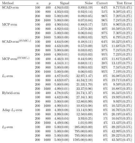
is {2−6, . . . ,23}. We use a=3.7 for the SCAD penalty and a= 3 for the MCP as suggested in the literature. We generate an independent test dataset of size n to report the estimated test error. The columns “Signal” and “Noise” summarize the average number of selected relevant and irrelevant covariates, respectively. The numbers in the “Correct” column summarize the percentages of selecting the exactly true model over replications.
Table 2.1: Simulation results for Model 1
Method n p Signal Noise Correct Test Error
SCAD-svm 100 400 4.94(0.03) 0.89(0.19) 64% 8.71%(0.4%)
100 800 4.93(0.03) 0.93(0.14) 51% 9.39%(0.4%) 200 800 5.00(0.00) 0.09(0.05) 96% 7.20%(0.2%) 200 1600 5.00(0.00) 0.07(0.04) 96% 7.24%(0.2%)
MCP-svm 100 400 4.90(0.04) 0.88(0.17) 53% 8.96%(0.4%)
100 800 4.92(0.03) 1.37(0.20) 40% 10.59%(0.5%) 200 800 5.00(0.00) 0.06(0.04) 97% 7.30%(0.2%) 200 1600 5.00(0.00) 0.09(0.03) 92% 6.79%(0.2%) SCAD-svm(SVMICγ) 100 400 4.64(0.08) 0.48(0.11) 64% 10.32%(0.6%)
100 800 4.63(0.09) 0.57(0.09) 52% 11.68%(0.7%) 200 800 5.00(0.00) 0.03(0.02) 97% 7.24%(0.2%) 200 1600 4.99(0.01) 0.05(0.03) 95% 7.23%(0.2%) MCP-svm(SVMICγ) 100 400 4.46(0.10) 0.44(0.08) 45% 11.81%(0.6%)
100 800 4.34(0.11) 0.68(0.11) 38% 13.13%(0.7%) 200 800 5.00(0.00) 0.09(0.03) 92% 7.34%(0.2%) 200 1600 5.00(0.00) 0.06(0.03) 95% 7.19%(0.2%)
L1-svm 100 400 4.87(0.05) 32.97(1.47) 0% 16.08%(0.5%) 100 800 4.63(0.07) 44.34(2.18) 0% 19.71%(0.6%) 200 800 5.00(0.00) 21.33(1.70) 0% 9.59%(0.3%) 200 1600 4.99(0.01) 33.37(0.96) 0% 10.88%(0.3%) Hybrid-svm 100 400 4.78(0.05) 24.74(1.37) 0% 16.34%(0.5%) 100 800 4.62(0.06) 27.16(1.30) 0% 19.93%(0.6%) 200 800 5.00(0.00) 12.86(0.99) 0% 9.93%(0.2%) 200 1600 4.99(0.01) 10.85(0.98) 0% 10.53%(0.3%) AdapL1-svm 100 400 4.39(0.08) 13.14(0.90) 0% 16.76%(0.5%) 100 800 3.99(0.08) 12.50(0.69) 0% 20.19%(0.6%) 200 800 4.86(0.04) 3.93(0.25) 1% 10.04%(0.3%) 200 1600 4.49(0.06) 1.01(0.09) 4% 13.43%(0.4%)
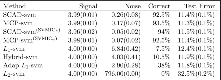
Table 2.2: Simulation results for Model 2 withn= 250 and p= 800
Method Signal Noise Correct Test Error
SCAD-svm 3.99(0.01) 0.26(0.08) 92.5% 11.4%(0.1%) MCP-svm 3.99(0.01) 0.17(0.07) 93.5% 11.3%(0.1%) SCAD-svm(SVMICγ) 3.96(0.02) 0.05(0.02) 94% 11.5%(0.1%)
MCP-svm(SVMICγ) 3.98(0.01) 0.07(0.02) 92.5% 11.4%(0.1%) L1-svm 4.00(0.00) 6.84(0.42) 7.5% 12.4%(0.1%) Hybrid-svm 4.00(0.00) 4.03(0.41) 10.5% 11.9%(0.1%) AdapL1-svm 4.00(0.00) 2.90(0.28) 38% 11.8%(0.1%)
L2-svm 4.00(0.00) 796.00(0.00) 0% 32.5%(0.2%)
signals when n = 100, but this is based on the fact that other methods select a much larger model without proper control of noise. A large proportion of the missed relevant covariates are from X1 as it has the weakest signal. Notice that SVMICγ performs almost the same as “pop-ulation tuning” whennis relatively large. In general, the non-convex penalized SVMs have an overwhelmingly high probability to select the exact true mode asnandp increase, while other methods show very weak, if any at all, ability to recover the exact true model. This is consistent with our theory of asymptotic oracle property of non-convex penalized SVMs. The test errors of SCAD- and MCP-penalized SVMs are uniformly smaller than those of any other method in all settings, even in the settings with a small sample sizen= 100 and tuned by SVMICγ, where they select slightly fewer signals. This is due to the fact that in high dimensional classification problem, a large number of falsely selected variables will greatly blur the prediction power of the relevant variables.
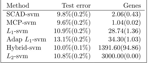
Table 2.3: Classification error of MAQC-II dataset
Method Test error Genes
SCAD-svm 9.8%(0.2%) 2.06(0.43) MCP-svm 9.6%(0.2%) 1.04(0.02)
L1-svm 10.9%(0.2%) 28.74(1.36) Adap L1-svm 13.1%(0.2%) 34.30(1.03) Hybrid-svm 10.0%(0.1%) 1391.60(94.86)
L2-svm 10.8%(0.2%) 3000.00(0.00)
to non-convex penalized SVMs, though its oracle property is largely unknown.
2.5
Real Data
We consider the MAQC-II data described in Section 1.2. The original data have been standard-ized for each predictor. To reduce the computational burden, only the 3000 genes with largest absolute values of the two samplet-statistics are used. Such simplification has been considered in Cai and Liu (2011). Though only 3000 genes are used, the classification result is satisfactory. We randomly split the data into an equally balanced training set with 50 samples with positive ER status and 50 samples with negative ER status. The rest are designated as the test set. As in the simulation study, we use a=3.7 for the SCAD penalty and a=3 for the MCP penalty. To get a fair comparison, a 5-fold cross validation is implemented on the training set to select a tuning parameter by a grid search over {2−15, . . . ,23} for all methods and the test error is calculated on the test data. The above procedure is repeated 100 times.
to 2576 genes across the 100 replications. Such stability is desirable, so that the procedure is robust to the random partition of the data. The numerical results confirm that SCAD- and MCP-penalized SVMs can achieve both promising prediction power and excellent gene selection ability.
2.6
Proofs
We first prove Lemma 2.1.
Proof of Lemma 2.1. Letl(β1) =n−1Pni=1Wi(1−YiZiTβ1)+. Note thatβb1= arg minβ1l(β1).
We will show that when ∀η >0, there exists a constant4such that for allnsufficiently large, Pr{inf||u||=4l(β01+
p
q/nu) > l(β01)} ≥1−η. Because l(β1) is convex, with probability at least 1−η, βb1 is in the ball {β1 : ||β1 −β01|| ≤ 4
p
q/n}. Denote Λn(u) = nq−1{l(β01+
p
q/nu)−l(β01)}. Observe thatE{Λn(u)}=nq−1{L(β01+
p
q/nu)−L(β01). Recall also that β0 = arg minβE{W(1−YXTβ)}. If we restrict the last p−q elements to be 0, it can be
easily seen that β01 = arg minβ1E{W(1−YZ
Tβ1)} = arg minβ
1L(β1), thus S(β01) = 0. By
Taylor series expansion of L(β1) around β01, we have E{Λn(u)} = 12uTH( ˜β)u+op(1), where
˜
β = β01+
p
q/ntu for some 0 < t < 1. As shown in Koo et al. (2008), for 0 ≤ j, k ≤ q,
the (j, k)-th element of the Hessian Matrix H(β01) is continuous given (A1) and (A2); thus
H(β) is continuous. By continuity of H(β) at β01, then 12uTH( ˜β)u = 12uTH(β01)u+o(1) as n → ∞. Define Wn = −
Pn
i=1ζiWiYiZi where ζi = I(1− YiZiTβ01 ≥ 0). Recall that
S(β01) =−E[ζiWiYiZi] = 0. If we define
Ri,n(u) =Wi(1−YiZiT(β01+
√ q √
nu))+−Wi(1−YiZ
T
iβ01)++ζiWiYiZiT
p q/nu
then we have
Λn(u) =E{Λn(u)}+WnTu/
√
qn+q−1
n
X
i=1
Then similar to Equation (28) in Koo et al. (2008) we have
q−2
n
X
i=1
E[|Ri,n(u)−E{Ri,n(u)}|2]≤C42E{q−1(1 +||Z||2)U(p1 +||Z||24pq/n)},
whereU(t) =I(|1−YiZT
iβ01|< t). (A2) implies that E{q−1(1 +||Z||2)}<∞. Hence, for any
>0, we can choose a positive constant C such that E[q−1(1 +||Z||2)I{q−1(1 +||Z||2)> C}]<
/2, then
E{q−1(1 +||Z||2)U(p1 +||Z||24p q/n)}
≤E[q−1(1 +||Z||2)I{q−1(1 +||Z||2)> C}] +CPr(|1−YiZiTβ01|< C4
p q/n).
We can take a large N such that Pr(|1 −YiZT
iβ01| < C4
p
q/n) < 2C for all n > N by (A4). This proves that q−2Pn
i=1E{|Ri,n(u)−E[Ri,n(u)]|2} → 0 as n → ∞. Observe that
E(WT
nu/
√
qn) = 0, and
Var (WT
nu/
√
qn)≤Cn−1q−1
n
X
i=1 (ZT
iu)2 ≤Cq−1λmax(n−1X
T
AXA)||u||2 →0
asn→ ∞. Therefore, the first term of (2.7) will dominate other terms asn→ ∞. By (A6) we have 12uTH(β
01)u > 0. Thus we can choose a sufficiently large 4 such that Λn(u) > 0 with probability 1−η for||u||=4and all sufficiently large n.
The proof of Theorem 2.1 relies on the following Lemmas.
Lemma 2.2.
Pr{ max q+1≤j≤pn
−1| n
X
i=1
WiYiXijI(1−YiZiTβ01≥0)|> λ/2} →0 as n→ ∞.
Proof. Recall thatE{WiYiXijI(1−YiZiTβ01≥0)}= 0. By (A5) and Lemma 14.9 of B¨uhlmann and Van De Geer (2011), we have Pr{n−1|Pn
i=1WiYiXijI(1 −YiZ
T
exp(−Cnλ2). Note that
Pr{ max q+1≤j≤pn
−1| n
X
i=1
WiYiXijI(1−YiZiTβ01≥0)|> λ/2}
= Pr{∪q+1≤j≤p{n−1| n
X
i=1
WiYiXijI(1−YiZiTβ01≥0)|> λ/2}} ≤pexp(−Cnλ2)→0
asn→ ∞ by the fact that log(p) =o(nλ2).
Lemma 2.3. For any 4>0,
Pr{ max
q+1≤j≤p sup
||β1−β01||≤4 √ q/n | n X i=1
WiYiXij[I(1−YiZiTβ1≥0)−I(1−YiZ
T
iβ01≥0)
−Pr(1−YiZiTβ1 ≥0) + Pr(1−YiZiTβ01≥0)]|> nλ} →0
as n→ ∞.
Proof. We generalize an approach by Welsh (1989). We cover the ball {β1 : ||β1 −β01|| ≤
4p
q/n} with a net of balls with radius 4p
q/n5. It can be shown that this net can be constructed with cardinalityN ≤dn4qfor somed >0. Denote theN balls byB(t1), . . . , B(tN),
wheretk, k= 1, . . . , N are the centers. Denoteκi(β1) = 1−YiZiTβ1, and
Jnj1 = N X k=1 Pr(| n X i=1
WiYiXij[I{κi(tk)≥0} −I{κi(β01)≥0} −Pr{κi(tk)≥0}+ Pr{κi(β01)≥0}]|> nλ/2), Jnj2 =
N
X
k=1
Pr( sup ˜
β1∈B(tk) |
n
X
i=1
WiYiXij[I{κi( ˜β1)≥0}
Then by (A5),
Pr( sup
||β1−β01||≤4 √
q/n
|
n
X
i=1
WiYiXij[I{κi(β1)≥0} −I{κi(β01)≥0}
−Pr{κi(β1)≥0}+ Pr{κi(β01)≥0}]|> nλ)≤Jnj1+Jnj2.
To evaluate Jnj1, let Ui = WiYiXij[I{κi(tk) ≥ 0} − I{κi(β01) ≥ 0} −Pr{κi(tk) ≥ 0}+
Pr{κi(β01)≥0}]. TheUi are independent mean-zero random variable , and Var(Ui) =E(Ui2) =
E(Ui2|Yi = 1) Pr(Yi = 1) +E(Ui2|Yi = −1) Pr(Yi = −1). Denote F and G the CDF of the conditional distribution ofZTβ
01 given Y = +1 and Y =−1. Observe that
E(Ui2|Yi= 1)≤C{Fi(1 +ZiT(β01−tk))(1−Fi(1 +ZiT(β01−tk))) +Fi(1)(1−Fi(1))
−2Fi(min(1 +ZiT(β01−tk),1)) + 2Fi(1)Fi(1 +ZiT(β01−tk))} ≤C|ZT
i(tk−β01)|,
and it follows by (A8) that
E(Ui2|Yi=−1)
≤C{Gi(−1 +ZT
i(β01−tk))(1−Gi(−1 +ZiT(β01−tk))) +Gi(−1)(1−Gi(−1))
−2(1−Gi(max(−1 +ZiT(β01−tk),−1))) + 2(1−Gi(−1))(1−Gi(−1 +ZiT(β01−tk)))} ≤C|ZT
i(tk−β01)|.
Thus we have n
X
i=1
Var(Ui)≤nCmax
i ||Zi||||tk−β01||=nO(
√
qlog(n))O(pq/n) =O(√nqlog(n)).
and C2 under the assumptions on the rate of λ,
Jnj1 ≤2Nexp(−
n2λ2/4
C1
√
nqlog(n) +C2nλ
)≤Cexp{4qlog(n)−Cnλ}. (2.8)
To evaluateJnj2, note that I(x≥s) is decreasing in s. Denote
Vi = [I{κi( ˜β1)≥0} −I{κi(tk)≥0} −Pr{κi( ˜β1)≥0}+ Pr{κi(tk)≥0}].
We have −Bi ≤Vi ≤Ai for any ˜β1 ∈B(tk), where
Ai = [I{κi(tk)≥ −4 p
q/n5} −I{κ
i(tk)≥0} −Pr{κi(tk)≥ 4 p
q/n5}+ Pr{κ
i(tk)≥0}],
Bi= [I{κi(tk)≥0} −I{κi(tk)≥ 4 p
q/n5} −Pr{κi(t
k)≥0}+ Pr{κi(tk)≥ −4 p
q/n5}].
Therefore, we have
Pr( sup ˜
β1∈B(tk) |
n
X
i=1
WiYiXij[I{κi( ˜β1)≥0} −I{κi(tk)≥0} −Pr{κi( ˜β1)≥0}+ Pr{κi(tk)≥0}]|> nλ/2)
≤Pr(Cmax
i |Xij|β˜ sup
1∈B(tk) |
n
X
i=1
Vi|> nλ/2)≤Pr{Cmax
i |Xij|max( n
X
i=1
Ai, n
X
i=1
Bi)> nλ/2}
by the fact that Ai >0, Bi>0. Note that n
X
i=1
Ai= n
X
i=1
[I{κi(tk)≥ −4 p
q/n5} −I{κi(t
k)≥0} −Pr{κi(tk)≥ −4 p
q/n5}+ Pr{κi(t
k)≥0}]
+ n
X
i=1
[Pr{κi(tk)≥ −4 p
q/n5} −Pr{κ
i(tk)≥ 4 p
and n
X
i=1
[Pr{κi(tk)≥ −4 p
q/n5} −Pr{κi(t
k)≥ 4 p
q/n5}]
=[Fi(1 +4pq/n5−ZT
i(β01−tk))−Fi(1− 4 p
q/n5−ZT
i(β01−tk))] Pr(Yi= 1) + [Gi(−1 +4
p
q/n5−ZT
i(β01−tk))−Gi(−1− 4
p
q/n5−ZT
i(β01−tk))] Pr(Yi=−1)
≤Cnlog(q)pq/n5√q=Clog(q)qn−3/2
by (A8). Denote
Oi=[I{κi(tk)≥ −4 p
q/n5} −I{κi(t
k)≥0} −Pr{κi(tk)≥ −4 p
q/n5}+ Pr{κi(t
k)≥0}].
Thus for sufficiently large n by λ=o(n−(1−c2)/2) and A(7), we have
N X k=1 Pr(C n X i=1
Ai> nλ/2)≤ N X k=1 Pr(C n X i=1
Oi > nλ/2−Clog(q)qn−3/2)≤ N X k=1 Pr(C n X i=1
Oi > nλ/4).
Notice that Oi are independent mean-zero random variables, and
E(O2i) =E[I{κi(tk)≥ −4 p
q/n5} −I{κ
i(tk)≥0}]2≤ p
q/n5max
i ||Zi||=Cqlog(n)n
−5/2,
using a similar idea to deriving the upper bound ofE(Ui2). Applying Bernstein’s inequality and the fact that maxi|Xij| = Op(
p
log(n)) for sub-Gaussian random variable, for some positive constantC1 and C2,
N
X
k=1
Pr(Cmax i |Xij|
n
X
i=1
Ai > nλ/2)≤Nexp(−
n2λ2/4
C1qn−3/2log(n)3/2+C2nλ
)≤Cexp{4qlog(n)−Cnλ}.
Similarly, we can prove thatPN
k=1Pr(Cmaxi|Xij|Pni=1Bi > nλ/2)≤Cexp{4qlog(n)−Cnλ}. Therefore, we have
Using (2.8) and (2.9), then the probability of Lemma 2.3 is bounded by p
X
j=q+1
(Jnj1+Jnj2)≤Cexp{log(p) + 4qlog(n)−Cnλ} →0 (2.10)
which completes the proof. Now we prove Theorem 2.1.
Proof of Theorem 2.1. The unpenalized hinge loss objective function is convex. By convex op-timization theorem, there existsvi∗ such thatsj(β) = 0b , j = 0,1, ....q, with vi=vi∗.
Note that min1≤j≤q|βˆj| ≥min1≤j≤q|β0j| −max1≤j≤q|βˆj−β0j|. Under Condition (A7), we haven(1−c2)/2min1
≤j≤qn|β0j| ≥M1, and max1≤j≤q|βˆj−β0j|=Op( p
q/n) by Lemma 2.1. Thus we have min1≤j≤q|βˆj|=Op(n−(1−c2)/2). Byλ=o(n−(1−c2)/2), we have Pr(|βˆj| ≥(a+12)λ)→1, , forj= 0,1, . . . , q.
By the definition of the oracle estimator, we have |βˆj|= 0, j = q+ 1, . . . , p. It suffices to show that Pr{|sj(β)b |> λ,for somej =q+ 1, . . . , p} →0. Let D={i: 1−YiZiTβb1 = 0}; then
forj=q+ 1, . . . , p, we have
sj(β) =b −n−1
n
X
i=1
WiYiXijI(1−YiZiTβ1b ≥0)−n−1 X
i∈D
WiYiXij(vj−1),
where −1 ≤ vi ≤ 0 if i ∈ D and vi = 0 otherwise. By (A5) (Zi, Yi) are in general positions, with probability one there are exactly (q+ 1) elements in D. Then by (A4), with probability one |n−1P
Pr{maxq+1≤j≤p|n−1Pni=1WiYiXijI(1−YiZiTβb1 ≥0)|> λ} →0. Observe that
Pr{ max q+1≤j≤p|n
−1 n
X
i=1
WiYiXijI(1−YiZiTβ1b ≥0)|> λ}
≤Pr{ max q+1≤j≤p|n
−1 n
X
i=1
WiYiXij[I(1−YiZiTβb1 ≥0)−I(1−YiZiTβ01≥0)]|> λ
2} + Pr{ max
q+1≤j≤p|n
−1 n
X
i=1
WiYiXijI(1−YiZiTβ01≥0)|>
λ
2}. (2.11)
By Lemma 2.2 the second term of (2.11) is op(1). Notice that from Lemma 2.1, the first term of (2.11) is bounded by
Pr[ max q+1≤j≤p|n
−1 n
X
i=1
WiYiXij{I(1−YiZiTβ1b ≥0)−I(1−YiZiTβ01≥0)}|> λ
2]
≤Pr[ max
q+1≤j≤p sup
||β1−β01||≤4 √
q/n
|n−1
n
X
i=1
WiYiXij{I(1−YiZiTβ1 ≥0)−I(1−YiZiTβ01≥0)
−Pr(1−YiZT
iβ1 ≥0) + Pr(1−YiZ
T
iβ01≥0)}|>
λ
4] + Pr[ max
q+1≤j≤p sup
||β1−β01||≤4 √
q/n
|n−1
n
X
i=1
WiYiXij{Pr(1−YiZiTβ1≥0)
−Pr(1−YiZT
iβ01≥0)}|>
λ
4]. (2.12)
By Lemma 2.3, the first term of (2.12) isop(1). Thus we only need to bound the second term of (2.12). Notice that
|Pr(1−YiZiTβ1 ≥0)−Pr(1−YiZiTβ01≥0)|
≤|Fi(1 +ZT
Then we have
max
q+1≤j≤p sup
||β1−β01||≤4 √
q/n
|n−1
n
X
i=1
WiYiXij{Pr(1−YiZiTβ1≥0)−Pr(1−YiZ
T
iβ01≥0)}|
≤Cmax
i,j |Xij| sup
||β1−β01||≤4 √
q/n
n−1
n
X
i=1
||Zi||||β1−β01||=Op(
p
logpn)O(pq/n)Op(
√
qlog(n))
=op(λ).
Thus
Pr[ max
q+1≤j≤p sup
||β1−β01||≤4 √
q/n
|n−1
n
X
i=1
WiYiXij{Pr(1−YiZiTβ1 ≥0)
−Pr(1−YiZiTβ01≥0)}|>
λ
4] =op(1),
which completes the proof. Now we prove Theorem 2.2.
Proof of Theorem 2.2. We will showβbis a local minimizer of Q(β) by writingQ(β) as g(β)− h(β).
By Theorem 2.1, we have Pr{G ⊆∂g(β)b } →1, where
G={ξ = (ξ0, . . . , ξp) :ξ0 = 0; ξj =λsgn(β)jb ), j= 1, . . . , q;ξj =sj(β) +λlj, j =q+ 1, . . . , p.},
wherelj ∈[−1,+1],j=q+ 1, . . . , p.
Consider any βin theRp+1 with the centerβband radius λ2. It is suffices to show that there
exist ξ∗∈ G such that Pr{ξ∗
j = ∂h(β)
∂βj } →1 as n→ ∞.
Since ∂h(∂ββ)
0 = 0, we haveξ
∗
0 = ∂h(β)
∂β0 .
Forj = 1, . . . , q, we have min1≤j≤q|βj| ≥min1≤j≤q|βˆj|−max1≤j≤q|βˆj−βj| ≥(a+12)λ−λ2 =
Pr{∂h(∂ββ)
j =λsgn(βj)} →1 for j= 1, . . . , q. For sufficently largen, sgn(βj) = sgn( ˆβj). Thus we
have Pr{ξ∗j = ∂h(∂ββ)
j } →1 as n→ ∞ forj= 1, . . . , q.
Forj=q+ 1, . . . , p, we have Pr{|βj| ≤ |βˆj|+|βj−βˆj| ≤λ} →1 by Theorem 2.1. Therefore we have Pr{∂h(∂ββ)
j = 0} → 1 for SCAD and Pr{
∂h(β) ∂βj = −
βj
a} → 1 for MCP. Observe that by Condition 2 we have Pr{|∂h(∂ββ)
j | ≤ λ} → 1 for the class of penalties. By Lemma 1 we
have Pr{|sj( ˆβj)| ≤ λ} → 1 for j = q+ 1, . . . , p. We can always find lj ∈ [−1,+1] such that Pr{ξj∗=sj( ˆβ) +λlj = ∂h(∂ββ)
j } →1 forj= 1, . . . , q, for both penalties. This completes the proof.
The proof of Theorem 2.3 consists of two parts. First we wil show that LLA algorithm initiated by ˜β(0) gives the oracle estimator after one iteration. Then we will show that once LLA algorithm finds the oracle estimator β, the LLA algorithm will find it again in the nextb
iteration, that is, the LLA algorithm will converge.
Proof of Theorem 2.3. Assume that none of the events Fni is true, fori= 1, . . . ,4. The proba-bility that none of these event is true is at least 1−Pn1−Pn2−Pn3−Pn4. Then we have
|β˜j(0)|=|β˜j(0)−β0j| ≤λ, q+ 1≤j≤p,
|β˜j(0)| ≥ |β0j| − |β˜j(0)−β0j| ≥aλ,1≤j≤q.
By Condition 2 of the class of non-convex penalties, we have p0λ(|β˜j(0)|) = 0 for 1 ≤ j ≤ q. Therefore the solution of the next iteration of ˜β(1) is the solution to the convex optimization
˜
β(1) = arg min
β n
−1 n
X
i=1
Wi(1−YiXT
iβ)++
X
q+1≤j≤p
p0λ(|β˜j(0)|)· |βj|. (2.13)
of subgradient, we have
n−1
n
X
i=1
Wi(1−YiXT
iβ)+≥n
−1 n
X
i=1
Wi(1−YiXT
iβ)+b + X
0≤j≤p
sj(β)(b βj−βˆj)
=n−1
n
X
i=1
Wi(1−YiXiTβ)b ++ X
q+1≤j≤p
sj(β)(b βj−βˆj).
Then we have for any β
{n−1
n
X
i=1
Wi(1−YiXiTβ)++
X
q+1≤j≤p
p0λ(|β˜j(0)|)|βj|} − {n−1
n
X
i=1
Wi(1−YiXiTβ)b ++ X
q+1≤j≤p
p0λ(|β˜j(0)|)|βˆj|}
≥ X
q+1≤j≤p
{p0λ(|β˜j(0)|)−sj(β)b · sgn(βj)} · |βj| ≥ X
q+1≤j≤p
{(1−1
a)λ−sj(β)b ·sgn(βj)} · |βj| ≥0.
The strict inequality holds unless βj = 0 for all q + 1 ≤ j ≤ p. Since we consider the non-separable case where the oracle estimator is unique, we know the oracle estimator is the unique minimizer of (2.13) and hence ˜β(1) = β. This proves that the LLA algorithm finds the oracleb
estimator after one iteration.
In the case that Fn2 is not true, we have |βˆj|> aλ for all 1 ≤j ≤q. Hence by Condition 2 of the class of penalties p0λ(|βˆj|) = 0 for all 1 ≤ j ≤ q and p0λ(|βˆj|) = p0λ(0) = λ for all
q+ 1≤j ≤p. Once the LLA algorithm finds β, the solution to the next LLA iteration ˜b β(2) is
the minimizer of the convex optimization problem
˜
β(2)= arg min
β n
−1 n
X
i=1
Wi(1−YiXT
iβ)++
X
q+1≤j≤p
λ|βj|. (2.14)
Then we have for any β
{n−1
n
X
i=1
Wi(1−YiXiTβ)++
X
q+1≤j≤p
λ|βj|} − {n−1
n
X
i=1
Wi(1−YiXiTβ)b ++ X
q+1≤j≤p
λ|βˆj|}
≥ X
q+1≤j≤p
and hence ˜β(2) = βb is the unique minimizer of (2.14). That is, the LLA algorithm finds the
oracle estimator again and stops.
Asn→ ∞, by Theorem 2.1 we havePn2→0 andPn4 →0. The proof forPn3→0 is similar to the proof for Theorem 2.1 by changing the constant to be (1−1a).
Now we prove Theorem 2.4.
Proof of Theorem 2.4. Let|| · ||1 be theL1 norm of a vector. Denoteln(β) =n−1Pni=1Wi(1−
YiXiTβ)++cn||β||1. Note that
E[np−1{ln(β0+pp/nu)−ln(β0)}] =E[np−1{W(1−YXT(β
0+
p
p/nu))+−W(1−YXTβ0)+}] +np−1cn(||β0+
p
p/nu||1− ||β0||1)
for some constant 4 that ||u|| =4. Observe that ||β0+pp/nu||1− ||β0||1 ≤ ||
p
p/nu||1 =
p
p/n||u||1. By the fact that cn = o(n−1/2), we have np−1cn(||β0+
p
p/nu||1− ||β0||1) → 0 as n → ∞. Then similar to the proof of Lemma 2.1, we can show that the expectation is dominated by 12uTH(β0)u > 0 and Pr{inf
||u||=4ln(β0+
p
p/nu) > ln(β0)} ≥ 1−η. Hence
||βbL1 −β0||=Op( p
p/n). Becausepn−12 =o(λ), Pr(|βˆL1
j −β0j|> λ, for some 1≤j ≤p) →0 as n → ∞. Then using Theorem 2.1 and Corollary 2.1 we have Pr{β(b λ) = βb} → 1, which
Chapter 3
Reliability Modeling for Dependent
Systems
This chapter is organized as follows. We introduce the problem and notation in Section 3.1. Section 3.2 summarizes the main results on the effects of dependence on system reliability and component importance and the extensions to multi-state systems. Implementation details are discussed in Section 3.3. Simulation studies are presented in Section 3.4, followed by the analysis of the stockpile test data in Section 3.5. The technical proofs can be found in Section 3.6.
3.1
Introduction
including components subjected to common stresses and components sharing a load. Models that ignore such sources of dependence are mis-specified and can result in biased estimates of system reliability and component importance. The assumption of component independence can limit the applicability of reliability modeling (Lawless, 1983).
In this chapter, we consider a system containing p components. In a binary system, each component has two states: functioning and failed. Define a binary random variable Xj as the state of the jth component, with Xj = 1 indicating the jth component is functioning, and
Xj = 0 indicating thejth component has failed,j = 1, . . . , p. The reliability of the component is denoted as πj = Pr(Xj = 1). Write X = (X1, . . . , Xp)T and π = (π1, . . . , πp)T. It is clear that if the components are mutually independent, the joint distribution of X is determined completely by the marginal probabilitiesπ.
Let XS denote a binary random variable representing the state of the system. As with the components, the system can be either in a functioning state or a failed state. We assume the state of the system is completely determined by the states of the components. That is, there exists a non-random mappingφ:{0,1}p→ {0,1}such thatX
S =φ(X). This functionφ(X) is called thestructure function of the system. Interest focuses on coherentsystems, which require certain regularity conditions on the structure function. A component isrelevant to the system if the structure function φ(X) is not constant in that component. The system is coherent if each component in the system is relevant and φ(X) is non-decreasing in each argument Xj,
j = 1, . . . , p. In this project, we only consider coherent systems. Some examples include the series system, withφ(X) =Qp
j=1Xj, the parallel system, withφ(X) = 1−
Qp
j=1(1−Xj), and the k-out-of-p system, with φ(X) = 1 if Pp
j=1Xj ≥k and φ(X) = 0 if
Pp
j=1Xj < k, where the system is functioning if and only if at least kout of p components are functioning.