High-throughput Data Modeling And Flexible Statistical Methods.

(1)

Abstract

HU, TAO. High-throughput Data Modeling And Flexible Statistical Methods. (Under the direction of Yi-Hui Zhou and Eric Laber.)

With the increased demands for analyzing large and complex data, it is critical to

integrate and explore effective methodologies and computational algorithms in the era

of Big Data. Big Data has been described as having the “four V” properties − Volume, Variety, Velocity and Veracity. This dissertation aims to explore those properties within

the background of modern data, and to develop novel and flexible frameworks which

accommodate some drawbacks of traditional statistical methods. First, a zero-inflated

beta-binomial model is described for modeling microbiome count data. This framework

introduces zero inflation to account for the excessive zero counts, and it can also handle both discrete and continuous phenotypes as well as other covariates. Thus, association

tests between microbiome community composition and phenotypes of interest can be

performed. A penalization method is also proposed to predict missing phenotypes based

on microbiome counts data. Second, three exact testing procedures are proposed for

SNP set analysis, which has been widely applied in analyzing next generation sequencing

(NGS) data. Comparing with single SNP testing, SNP set analysis is able to detect

signals by examing groups of SNPs together. Traditional testing procedures are based on

asymptotic null distribution of the test statistic, but they are not valid for small sample

sizes. The proposed exact tests will achieve high power even when sample size is small. To solve the computation bottleneck issue for exact testing methods, computationally

efficient algorithms are derived and implemented into a user friendly software. Finally,

an approximate Thompson sampling strategy is proposed for streaming data analysis.

Streaming data is characterized as accumulating properties and high complexity. The

proposed strategy is a model-based planning algorithm, and is designed to balance the

exploration-exploitation trade-off which is caused by the unknown environment.

Ap-proximate Thompson sampling enables us to estimate the system dynamics and optimal

policy that give best rewards at the same time. Asymptotic convergence rates are derived

(2)

c

(3)

High-throughput Data Modeling And Flexible Statistical Methods

by Tao Hu

A dissertation submitted to the Graduate Faculty of North Carolina State University

in partial fulfillment of the requirements for the Degree of

Doctor of Philosophy

Bioinformatics with Co-Major in Statistics

Raleigh, North Carolina

2017

APPROVED BY:

Yi-Hui Zhou

Co-chair of Advisory Committee

Eric Laber

Co-chair of Advisory Committee

Fred Wright Brian Reich

(4)

Dedication

(5)

Biography

Tao Hu was born in Xinyu, Jiangxi Province, China in 1989. He completed his Bachelor’s

degree in Bioinformation Technology from Huazhong University of Science and

Technol-ogy, Wuhan, China, in June 2011. After graduation, he worked as an internship at

Shanghai Center for Bioinformation Technology, Shanghai, China, and mainly focused

on gene prediction and other bioinformatics analyses. In August 2012, he enrolled at

North Carolina State University, Raleigh, NC, USA, to pursue his doctoral degree in Bioinformatics. In 2013, he decided to take Statistics as co-major.

His research interests include statistical modeling, machine learning and statistical

(6)

Acknowledgements

First I would like to thank my co-advisors, Dr. Yi-Hui Zhou and Dr. Eric Laber. Thanks

for their precious guidances and supports. They not only led me into the world of data

analysis and showed me the beauty of research, but also taught me how to overcome

difficulties in my academic life , even my daily life. Their passions and dedications at

work and research will inspire me forever.

I would also give my sincere appreciation to my committee members Dr. Fred Wright, Dr. Brian Reich and Dr. David Reif for their valuable comments and suggestions. I

especially thank Dr. Fred Wright for his helps in improving my research and dissertation.

I also want to thank all the professors, who taught me at NC State, for imparting their

knowledge to me.

I also would like to thank Dr. Hua Zhou from University of California, Los Angeles

and Dr. Jin Zhou from University of Arizona for their guidances in the project “Exact

variance component tests of SNP sets”.

I would like to say thank you to many colleagues and friends, Nick Meyer, Cai Li,

Yuelong Guo, Xiang Ji, Yiwen Luo, Jihe Liu, Kuangyu Wang. Thanks for their insightful discussions and sharing their research experiences.

As always, I wish to express my deepest gratitude to my beloved family. Their caring,

support and love is the source of my motivation.

Last but certainly not least, I would like to thank my wife, Shuzhen Kuang, for her

ceaseless understanding, patience, encouragement, companionship and love. She comforts

(7)

List of Tables

Table 2.1 Type I errors for discrete case at level α= 0.05 . . . 29 Table 2.2 Type I errors for continuous case at levelα = 0.05 . . . 29 Table 2.3 Top 10 OTUs discovered by different methods. Note that “cstr”

stands for constrained modeling. Values in brackets are q-values adjusted by FDR. . . 40

Table 3.1 Empirical type I error rate of eScore, eLRT, and eRLRT based on 106_simulation replicates. Top panel shows the cases when simulation region include both common and rare, while bottom panel shows the cases when only rare variants are included. . . 54 Table 3.2 Models (Scenarios) for simulating phenotypes for power

compar-isons, based on a 10kb region of the haplotype pool from the SKAT software. . . 55 Table 3.3 The number of gene sets that pass genome-wide significant level

at FWER 0.05 from the COPDGene exome sequencing study. For eScore, eRLRT, eLRT, and SKAT, linear kernel and no weights are adopted. . . 60 Table 3.4 The number of gene sets that pass genome-wide significant level

at FWER 0.05 from the COPDGene exome sequencing study. For eScore, eRLRT, eLRT, and SKAT, linear kernel and no weights are adopted. . . 61 Table 3.5 Runtimes (in seconds) of different methods for the COPDGene data

analysis. . . 61

(10)

(11)

List of Figures

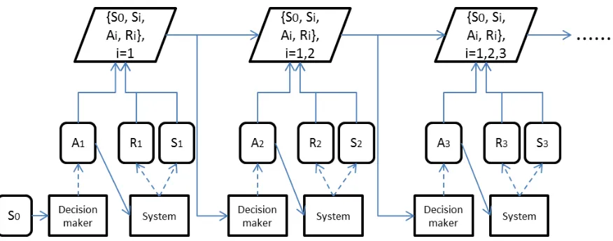
Figure 1.1 Visualization of streaming data. Si represents the state

informa-tion, Ai represents actions decision maker administer and Ri

rep-resents outcome. . . 6

Figure 2.1 Fittings of microbiome count data for taxaLactobacillus.vaginalis under different models in “ravel” dataset. Panel (a) is the his-togram for original data. Panel (b)-(f) are hishis-tograms of fittings under corresponding models. . . 15

Figure 2.2 Power plots under different scenarios . . . 31

Figure 2.3 Comparing estimated standard deviation and bootstrapping stan-dard deviation ofβ1i for discrete case. . . 33

Figure 2.4 Comparing estimated standard deviation and bootstrapping stan-dard deviation ofβ1i for continuous case. . . 34

Figure 2.5 The plots of mean-variance relationship and OTU group correla-tions for simulated data. . . 35

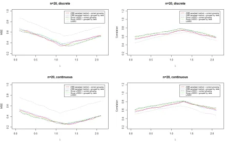
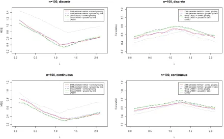
Figure 2.6 Prediction results when sample size is 20. . . 36

Figure 2.7 Prediction results when sample size is 100. . . 37

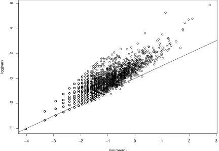
Figure 2.8 Mean-Variance plot on the log scale of the real dataset. . . 39

Figure 2.9 Prediction results for soil microbiome data. . . 41

Figure 3.1 Discrepancy between SKAT and eScore p-values. Left: there is no SNP set effect (null model,σ2 g = 0). Right: there is SNP set effect (alternative model,σ_g2 = 0.5). . . 52

Figure 3.2 Power comparison when causal variants are both common and rare (Models I-III). Left panel shows the power when 10% of the variants in the testing region are causal; right panel shows the power when 30% of the variants in the testing region are causal. Heritability is fixed at 10%. . . 56

(12)

(13)

Chapter 1 Introduction

1.1 Motivation

With the develepment of technology, we are able to generate large amounts of data which is high volume or has high “velocity”, meaning that it is generated quickly. There is

grow-ing popularity to use the term “Big Data” to represent such data and the correspondgrow-ing

analytical methods (Lynch, 2008; Marx, 2013; Cavanillas et al., 2016). High volume

in-dicates that the size of data is much larger. For example, high-throughput sequencing

technologies (Metzker, 2010; Reuter et al., 2015), which are powerful tools in genomics

studies, can quantify hundreds of thousands of genes at a time and then pull out the

massive information for stream down analysis. At the same time, hardware and software

solutions have been proposed to accommodate the increasing requirement of storing and

processing such big data (Shvachko et al., 2010; Zhang et al., 2010; Saecker and Markl,

2013). High velocity indicates that the data is accumulating and available in real-time. As a comparison, traditional data analysis procedures employ statistical methods (linear

regression, machine learning techniques, and so on) to a training data set, which is

ob-served and fixed. The high velocity property is becoming common in many fields. For

example, in data-driven management of infectious diseases, the information about the

spread of disease is accumulating and all historical information can be used to decide

how to assign treatments (Chad`es et al., 2011). Both high volumn and high velocity

data provide us a deeper insight of the objects and give us the opportunity to decipher

unknown realms.

(14)

theories have developed so maturely that they become the routines for data analysis,

methods for Big Data are still in early stages. We may need to make restricted or even

impractical assumptions to ensure ordinary methods work (Fan et al., 2014; Gandomi

and Haider, 2015). Also, the data cleaning, handling of missing data, and other quality

control issues could be nontrivial (Graham, 2009; Jagadish et al., 2014). Three important

questions are: 1) will ordinary methods be applicable to Big Data problems? 2) if not,

can we develop new statistical methods which are suitable for Big Data problems? 3)

are there statistical theories that guarantee the performances of those methods?

In this dissertation, we focus on high-throughput ‘omics data and streaming data. The

objectives are to develop new modeling methods, computational efficient algorithms, and statistical theories for these data. For high-throughput ‘omics data, we focus specifically

on microbiome count data and single-nucleotide polymorphism (SNP) data, and explore

them with two types of analytics: discovery modeling and predictive modeling (Shmueli,

2010). Discovery modeling aims to reveal knowledge from the observed data, while

pre-dictive modeling attempts to find out what unobserved data should look like. Streaming

data comes in sequentially and the underlying data generation process is unknown in

many situations (Litvin et al., 2013; Fackler and Pacifici, 2014). That data is complex

because it accumulates rapidly over potentially infinite time horizon, also called high

dimensional, or it is composed of a single data point at each time stage.

1.2 Introduction to data types

1.2.1 Microbiome count data

The human microbiome is a collection of all microbes (e.g., bacteria, fungi, and viruses)

at human body sites (Cho and Blaser, 2012). Usually we are interested in the collection

of microbes in a specific human site, such as gut, oral cavity, skin, etc. The species of

microbes are different across organisms, and across humans. The human microbiome has

10 times more bacterial cells than human cells, and collectively 1,000 times more genes than the human genome (Whitman et al., 1998; Consortium et al., 2012). Therefore,

the human microbiome can be considered an extension of the human genome. Due

to its huge magnitude, the human microbiome plays important roles in human health

(Clemente et al., 2012; Johnson and Versalovic, 2012; B¨ackhed et al., 2005). For example,

(15)

produce vitamins that human genes can not synthesize, and so on. More recently, studies

indicate that the human microbiome has a vital impact on human diseases, such as

diabetes (Qin et al., 2012), obesity (Turnbaugh et al., 2009) and HIV (Lozupone et al.,

2013).

Traditional methods for studying microbiome is cultudependent, which means

re-searchers need to cultivate an organism selectively in lab and then detect the microbes

in it. However, traditional methods are low-throughput and the vast majority of

mi-crobes can not grow in lab. Taking advantage of modern high-throughput sequencing

technologies, researchers are able to directly sequence the extracted DNA (i.e., without

lab cultivation) at a genome-scale, thus make it possible to reveal the diversity of micro-bial communities. Modern microbiome studies based on high-throughput sequencing are

parts of metagenomics (Riesenfeld et al., 2004).

Currently, there are two major sequencing strategies for microbiome studies: 16S

rRNA gene profiling (Consortium et al., 2012) and shotgun metagenomic sequencing

(Tringe et al., 2005; Liu et al., 2011).

• 16S rRNA gene profiling

In order to figure out the composition of a microbiome, we need to distinguish

each distinct genome. Since sequencing every letters for all genomes is impractical

and unnecessary, there exist molecular markers that help us uniquely identify a

genome. One of the most popular markers is the 16S ribosomal RNA (rRNA) gene

with 1.5Kbp length. The 16S rRNA gene is present in all bacteria genomes, so

no genomes will be missed, and it contains both conserved regions and variable

regions, which can be used to cluster the components of a microbiome.

The 16S rRNA gene profiling method begins with sequencing all 16S sequences. Then the 16S sequences can either be searched with 16S databases or clustered

based on the variable regions. The resulting clusters are called Operational

Taxo-nomic Units (OTUs). Each OTU can be roughly thought of as a species.

• shotgun metagenomic sequencing

The basic principle is to break extracted DNA sequences from the sample into small

pieces, sequence all those short sequences and then reconstruct them into original

sequences. Researchers can obtain all genes and the abundance of microbes present

(16)

is still a big challenge (Sharpton, 2014). For example, binning (assign metagenomic

sequence to a taxa) and assembly (combine the reads from the same genome region

into a contig).

In this dissertation, we will focus on the 16S rRNA sequencing data, although the basic approach is applicable to full-genome sequencing data. Typically, the data is represented

by a count matrix, with rows represent samples and columns represent OTUs. In the rest

of this dissertation, we will use the term “microbiome count data” to represent 16S rRNA

sequencing data. As the development of modern sequencing technologies, the number of

OTUs is large, usually on the scale of 103 _{- 10}5_{. Other than the OTU counts, microbiome} count data usually come with several covariates for each sample. The covariate can be

discrete (for example, group indicator) or continuous (for example, phenotypes).

The main interest for this type of data is to test the effects of certain covariates

(usually phenotypes) to the composition of microbiome count data while adjust other confounders. The effects can be different across OTUs, and thus we are interested in

finding covariates which are correlated with each single OTU. Essentially, it is discovery

modeling for each OTU. We use the term “discovery study” to represent such study,

and similar methology can be applied to other count data, for example, RNA-Seq data

(Marioni et al., 2008; Robinson and Oshlack, 2010; Anders and Huber, 2010). In practice,

many phenotype values are missing. Thus, another interest is to predict the missing

phenotypes based on counts information and any other covariates. We use the notion

“prediction study” to represent such study.

1.2.2 SNPs data

Single-nucleotide polymorphism (SNP) is a single nucleotide variation in DNA sequence

within a population. SNPs are the most common type of genetic variation among people, about one in 1000 letters of human DNA vary in the form of a SNP. The letters in human

DNA sequences are also known as nucleotides. The four possible letters are A (adenine),

C(cytosine), G(guanine), and T (thymine), and they are linked to a phosphodiester

backbone to construct a DNA strand. Thus, a SNP, for example, could be replacing

letter C with letter T in a DNA strand. Though SNP doesn’t always mean abnormal,

certain SNPs are landmarks for pinpointing disease-causing genes (de Bakker et al., 2006;

(17)

There are three types of biological techniques to measure the SNPs: (1)

Hybridization-based methods using the biology of complementarity to hybridize DNA probes to the SNP

site, and obtaining the Polymerase chain reaction (PCR) products of hybridization, we

can check the physical or chemical properties of the PCR product to determine the

ex-istence of SNP. A modern version is to utilize microarrays to interrogate many SNPs

simultaneously; (2) Enzyme-based methods make use of restriction endonucleases, which

possess high affinity to unique restriction sites. Use such restriction endonucleases to cut

the DNA sequences, and run a digestion on the resulting genomic subsequences. A larger

subsequence indicates the existence of SNP; (3) Direct sequencing methods are not

avail-able until last decades due to development of sequencing technology. Next-generation sequencing technology is a population method to measure the genotypes directly and

thus locate the SNPs. The type of SNP data we consider here is usually represented by

genotype matrix, with rows represent individuals and columns represent SNPs.

Covari-ates are also available for each individual.

The main interest for this type of data is to associate SNPs with interested phenotype

(for example, disease). The idea to use a linear model, and estimate the SNP effects either

as fixed or random effects. Instead of testing SNP one by one, researchers tend to examine

group of SNPs at a time. This is called SNP set analysis (Fridley and Biernacka, 2011).

We use the term “discovery for per-set analysis” to represent such study. Grouping SNPs make sense because a disease is usually effected jointly by multiple SNPs.

1.2.3 Streaming data

The streaming data considered here is accumulating along time stages. A visualizing of

streaming data is shown in in figure 1.1. The data generation process can be summarized

as follows: imagine there is a unknown system/environment and a decision maker who will

interact with the system. At each time stage, decision maker observes state information of

the system. Based on the state information and all history information collected during

previous time stages, the decision maker administers an action to the system, and an

outcome will be given as feedback. Thus, the data at each single time stage is a tuple

of state information, action and outcome. For example, in the context of mobile-health, data collected actively through a mobile device can be used to monitor a patient’s health

status and thus to inform an individualized treatment strategy that applies appropriate

(18)

Figure 1.1: Visualization of streaming data. Si represents the state information, Ai

represents actions decision maker administer andRi represents outcome.

The objective is to construct decision support system that map cumulatived data to

a decision such that mean cumulative utility, which is certain function of outcome, will

be maximized with respect to all time stages. The key feature of this task is that we do

not know the system dynamics model that generates the state information or outcome. Thus, the estimation of decision support system and system dynamics model must be

done simultaneously and in real-time. And there is a traoff between estimated

de-cision support system that lead to a large gain in information about system dynamics

model with those that would maximize mean cumulative utilities based on current

es-timated system dynamics model. This is known as exploration-exploitation trade-off in

reinforcement learning (Kaelbling et al., 1996; Sutton and Barto, 1998).

1.3 Existing methods in general

1.3.1 Common strategies for discovery and prediction studies

Modern discovery and prediction problems always fit into the framework of high-dimensional

data analysis, in which number of features p is greater than sample size n. Canonical

asymptotic theorems handle the case when sample sizen goes to infinity, and many

well-established methods have been developed. There are mainly two types of high-dimension:

(19)

(HDLSS); (2) _np →constant, and p, n→ ∞. The theory of random matrices is the foun-dation to solve this problem. In this dissertation, we consider microbiome count data

and SNP data, in which the number of features are much more than sample size, they

are both high-dimensional. For microbiome count data, features are OTUs, and for SNP

data, features are the SNPs.

Popular methods for modeling microbiome count data are assuming certain

distri-butions for count data and then linking them with phenotypes of interest and other

covariates. Poission (Min and Agresti, 2005) and negative binomial (Fang et al., 2014)

are two population choices for the count distribution. And examples for linking count

data with phenotypes include generalized linear models and generalized linear mixed models (Li, 2015; Chen and Li, 2016).

SKAT (sequence kernel association test) is one of the most popular tool for SNP set

analysis (Wu et al., 2011). SKAT employs generalized linear mixed model (GLMM) and

uses quadratic form to test the random effects of SNP set, and assumes a mixture

chi-squared distribution as p-value’s asymptotic null distribution. Other methods include

burden tests (Price et al., 2010).

In our knowledge, there is little systematic works on the prediction problem in the

context of microbiome count data. The prediction problem considered here is similar

as quantitative trait prediction (Yi and Xu, 2008; De Los Campos et al., 2009; Mackay et al., 2009). However, due to the special characteristics of microbiome count data, those

methods may not be appropriate.

1.3.2 Common strategies for streaming data

The problem of decision support system estimation considered here belong to a broad

class of data-driven decision making (Power et al., 2015). A popular formulization of

data-driven decision making is Markov decision process (Howard, 1960). The core idea

of Markov decision process is to find an optimal policy, which maps state information

to decision, such that long term rewards are maximized. Standard algorithms for

esti-mating Markov decision process include policy iteration (Howard, 1960; Iyengar, 2005),

policy search(Robins et al., 2008; Zhang et al., 2012), and Q-learning (Murphy, 2003; Laber et al., 2014). This estimation problem is also similar to estimation of dynamic

treatment regime, which aims to construct individualized treatment allocation strategy

(20)

of dynamic treatment regime algorithm that it is designed for independent, identically

distributed data in simple settings (for example, finite time horizon, and the estimation

is offline), prevent its directly application to our settings.

As a tool to handle the exploration-exploitation trade-off, Thompson sampling was

proposed originally for multi-armed bandit problems and has been studied extensively

recently years (Agrawal and Goyal; Russo and Van Roy, 2014; Gopalan et al., 2014). The

key idea of Thompson sampling is to compute a posterior distribution over the optimal

policy at each time stage, and choose the policy that maximize mean cumulative utility

over the posterior distribution as current estimation (Thompson, 1933; Scott, 2010).

Gopalan and Mannor (2015) applied Thompson sampling to Markov decision processes for the first time. Thus, there are accumulating evidences indicating that Thompson

sampling has great potential to handle general decision-making problems.

In our settings, an important perspective is that decision makers have to interact with

the system or environment in order to receive feedback, and that feedback will further

help to construct a better decision support system. In many cases, the system dynamics

are unknown, i.e., we only observe the final feedback but have no idea about how the

feedback is generated. A common way to handle this issue is using model-based planning

algorithm (Sutton and Barto, 1998). Model-based planning algorithm require a informed

model for the system dynamic. During each iteration, we will seek the optimal policy under an updated estimator for the system dynamics. Therefore, estimations for the

optimal policy and system dynamics are processed at the same time, which turn out to

be exactly the same as the exploration-exploitation trade-off.

1.4 Challenges with the data

Though many studies have been conducted to analyze the data types which are focused

on here, there are still several challenges:

• Microbiome count data

With similar properties as RNA sequencing data, microbiome data is also count

data. An important characteristic of microbiome data is its excessive zero counts,

beyond that prediction from a standard count model, even with overdispersion.

If we apply statistical methods designed for RNA seqiencing data directly, they

(21)

we develop a method that borrows the information from the data itself or other

side information. As a result, that method should be able to model the data more

precisely.

Another issue is that when missing data appear, popular practice is to throw the

missing data away or impute them by naive methods, seldom researches are about to handle this missing data problem in microbiome data, let along the statistical

properties of those methods (for example, the coverage and mean squared error).

• SNPs data

SNP set tests are classical and powerful method for analyzing next generation sequencing data. But the popular Sequence Kernel Association Test (SKAT) is not

appropriate for small or median sample size, becasue SKAT computes p-value base

on asymptotic properties. Thus, it is necessary to design testing procedure which

is suitable for small size.

Besides that, testing variance components in linear mixed model is computationally

challenge, especially when scale it to genome-wide studies (Zeng et al., 2014, 2015).

Thus, it is important to develop computationally efficient algorithm to this problem.

• Streaming data

Streaming data is complicated in the way that the data are either: (i) accumulating

rapidly over an indefinite time horizon; (ii) high-dimensional; or (iii) composed

of a single data stream, i.e., no independent replication. We need to adjust our

estimations time by time when new data come in or out.

Existing methods for dynamic treatment regimes can not be applied directly

be-cause their estimation procedures are offline and they are designed for independent,

identically distributed data, while the streaming data is accumulating and we can

only observe a single replicate of the data.

Thompson sampling is a powerful tool to balance exploration and exploitation for

multi-armed bandit problem. however, existing methods about Thompson

sam-pling are designed for relatively simple settings. In our decision support system

estimation problem, the settings are more complexed because: (i) the number of

possible decisions is too large to enumerate; (ii) compute draws from posterior

(22)

very large that existing solutions can not fit. What’s more, we are especially

inter-ested in the asymptotic properties of Thompson sampling type algorithm. Instead

of measured by empirical experiments, we want to develop statistical theories about

the convergence rates of the algorithm.

1.5 Contributions and organizations

Chapter 1 introduces the motivation and data types this dissertation focus on, as well as

issues with statistical methods for those data types.

Chapter 2 describes a zero-inflated beta-binomial model for microbiome count data. It

introduces zero inflation probability to account for the excessive zero counts and propose

a polynomial relationship between over-dispersion parameter and sample mean, as well as

prediction methods for microbiome data. Asymptotic result for the proposed prediction

algorithm is also derived.

Chapter 3 describes three exact tests for testing SNP set random effect in linear mixed

model, and implement computationally efficient software for use.

Chapter 4 describes approximate Thompson sampling for streaming data, and derives

(23)

Chapter 2 Zero-inflated Beta-binomial Model

for Microbiome Count Data Analysis

2.1 Introduction

The human microbiome consists of the collection of all microbes at sites in or on the

human body (Cho and Blaser, 2012), with 10 times more cells than the human host,

and representing 1000-fold greater diversity of genes (Whitman et al., 1998; Consortium

et al., 2012). Many studies have shown that microbial communities play an important

role in maintaining health for the host species (B¨ackhed et al., 2005; Turnbaugh et al.,

2009; Clemente et al., 2012; Qin et al., 2012). Therefore, deciphering the composition

of the microbiome and its association with phenotype (for example, disease status) is critical in understanding biological mechanisms.

Traditional methods for studying microbiomes have been culture-dependent and

low-throughput, as the vast majority of microbes cannot be easily isolated and grown. With

modern high-throughput sequencing and a metagenomic approach (Riesenfeld et al.,

2004), investigators can now directly sequence the extracted DNA of an entire

micro-biomal community, revealing the diversity of microbial communities. A common

se-quencing strategy (Consortium et al., 2012) is to sequence only the 16S ribosomal RNA

(rRNA) gene, which is highly specific to bacterial species. The 16S rRNA sequences

can be grouped into different clusters called Operational Taxonomic Units (OTUs), or taxa. The data are represented by a sequence count matrix, organized here with rows

(24)

In the past decade, a number of methods have been developed for microbiome count

data analysis. Those methods aim to explore the associations between phenotypes of

interest and the microbiome counts. We will refer to such method as discovery study

throughout the paper. Distance-based analysis (McArdle and Anderson, 2001; Lozupone

and Knight, 2005; Chen et al., 2012) is one popular approach to associate overall

mi-crobiome composition with phenotypes. The basic strategy is to compute the pairwise

distance matrix among samples using a specific metric, and then apply downstream

anal-yses to these distances. For analanal-yses by OUT, a logistic normal multinomial regression

model (LNM) (Xia et al., 2013) has been used, assuming the count data came from a

multinomial distribution given the underlying composition of OTUs, while the composi-tions are modeled with a logistic normal distribution. MiRKAT (Zhao et al., 2015) is a

kernel-based regression model, where microbiome compositions are included in the

ker-nels, and the phenotype is regressed on the kernels and other covariates. A more recent

method employs a zero-inflated Gaussian distribution (ZIG) (Paulson et al., 2013).

In a discovery study, the goal is to perform association testing between the microbiome

count data versus the included phenotype, which can NOT be missing. However, it is

common that some phenotype values are missing, or that we may be interested in future

(unobserved) phenotypes. In this case, we may be interested in imputing/predicting the

missing phenotype values from the microbiome count data. We will call such imputation effort as aprediction study. To our knowledge, there is little existing systematic research

on prediction methods designed specifically for microbiome count data. A trivial idea

is to apply existing data imputation methods on the microbiome count data directly.

However, these methods do not consider the unique characteristics of microbiome count

data.

Although the recently developed methods have appealing properties, it remains

im-portant to conduct basic analyses at the feature (OTU) level. Direct modeling of

mi-crobiome count data versus phenotype typically uses generalized linear models (GLMs),

which typically must account for overdispersion (Anders and Huber, 2010; Xu et al., 2015; Weiss et al., 2015), and for which methods developed for RNA sequence (RNA-Seq) data

may be appealing. For example, the negative binomial modeling in edgeR (Robinson

et al., 2010) has been applied on micriobiome data with phyloseq (McMurdie and Holmes,

2014). BBSeq (Zhou et al., 2011b) employs a beta-binomial model for the count data

(25)

relationship. However, directly employing RNA-Seq data analysis methods may be

prob-lematic because microbiome count data is usually sparse ,with many zero counts (Weiss

et al., 2015). Accordingly, zero-inflated negative binomial models (ZINB) Fang et al.

(2014) have also been proposed, but do not allow for arbitrary covariates.

Here, we summarize the major challenges of analyzing microbiome count data as: 1)

microbiome count data has excessive zero counts; 2) there usually exist special structure

with the data (Zhou et al., 2011b), and fail to consider it may lead to bad results; 3) there

is still lack of flexible software to conduct the analysis; and 4) there is little systematic

research on predicting missing phenotypes. Existing methods are designed to handle one

or several challenges above, but not all of them. In this paper, we intended to propose a framework which handle all the challenges at the same time.

Specifically, we propose a framework that can be used for both discovery and

predic-tion studies. First, we present a zero-inflated beta-binomial model (ZIBB) to explore the

association between phenotypes/covariates and microbiome count data. The ZIBB model

assumes the count data distribution consists of a mixture of a point mass probability at

zero, and a beta-binomial distribution (which may have an appreciable additional mass at

zero). Our proposed method is an extension of the beta-binomial model of BBSeq (Zhou

et al., 2011b). ZIBB models the effects of phenotypes on the microbiome data counts,

as well as the effects of other covariates on the zero counts probability. A Wald statistic is used to test statistical significance of the phenotype while accounting for covariates.

Second, we propose a prediction algorithm for imputing the missing phenotype values.

Our prediction algorithm formulate the corresponding parameter estimation problem as

solving a penalized GLM, and then calculate a posterior mean as final prediction based on

Bayes rule. We also demonstrate the asymptotic properties of our prediction algorithm.

The proposed framework has the following advantages over canonical methods:

(i) ZIBB assumes that the count distribution is beta-binomial, which has a clear

two-stage interpretation that each count follows a binomial distribution for a varying success probability that itself is a beta random variable. The success probability

has a clear interpretation, i.e., as proportional to the compositional proportion of

an OTU at a sample.

(ii) ZIBB also employs logistic regression to model the zero point mass probability as a

function of covariates. The approach is important to provide additional flexibility

(26)

(iii) Using the same strategy as BBSeq (Zhou et al., 2011b), ZIBB considers a

con-strained approach to model the over-dispersion as a polynomial function of the

systematic (mean) component of the GLM. The constraint follows the observation

that sample overdispersion estimates are often strongly correlated with the sample

mean for real count data, including microbiome data. Simulations will show that

the constrained approach indeed increases the power of our method compared to

competing methods.

(iv) We propose a prediction algorithm under the assumptions of the ZIBB model. This

prediction algorithm take advantage of ZIBB modeling for microbiome count data, and it is easy to interpret if we assume the ZIBB model.

(v) An R package, ZIBBSeq, is implemented. This package aims to provide user friendly

pipelines for analyzing the microbiome count data. It simplify the analyzing

proce-dure for researchers, especially for who are not that familiar with statistical

meth-ods. This package is also helpful for experienced researcher, as it packed useful

functions and facilitate the researches to focus more on the higher level other than

the calculation details.

Last, the simulations and real data analysis demonstrate that the proposed ZIBB

based approach performs well for microbiome data analysis.

2.2 Methods

2.2.1 Why we need a zero-inflated model

The two major improvements of our proposed framework are 1) employing zero-inflated

modeling and 2) considering a constrained approach to estimate the over-dispersion

pa-rameters. To illustrate that those two improvements are necessary, we extracted count

data of taxon Lactobacillus.vaginalis from a dataset we termed “ravel” (Ravel et al.,

2013) and fit it with different models (Figure 2.1). Figure 2.1.a is the histogram of

origi-nal microbiome count data for the taxon Lactobacillus.vagiorigi-nalis, Figure 2.1.b-Figure 2.1.d

are the histograms of fittings under Poission, ZIP and ZINB models, and Figure

2.1.e-Figure 2.1.f are the histograms of fittings under our proposed method: 2.1.e-Figure 2.1.e is

(27)

a. Original data Counts Propor tion 0 20 40 60 80 100

0 5 10 15 20 25 >30

b. Poission model

Counts Propor tion 0 20 40 60 80 100

0 5 10 15 20 25 >30

c. Zero−inflated Poission model

0 5 10 15 20 25 >30

d. Zero−inflated Negative Bionomial model

0 5 10 15 20 25 >30

e. Zero−inflated Beta−bionomial free model

0 5 10 15 20 25 >30

f. Zero−inflated Beta−bionomial constrained model

0 5 10 15 20 25 >30

Figure 2.1: Fittings of microbiome count data for taxaLactobacillus.vaginalis under dif-ferent models in “ravel” dataset. Panel (a) is the histogram for original data. Panel (b)-(f) are histograms of fittings under corresponding models.

result after imposing the constraint. Compared to Figure 2.1.b, Figure 2.1.c, and

Fig-ure 2.1.d, zero-inflated models evidently provide a better fit for the data, while Poisson

model fitting leads to an unrealistically lower proportions of zero counts. Our proposed

method with constrained approach provides the most realistic fit, which is suggestive of

the improved performance when using a separate model to constrain the over-dispersion parameters. Below we conduct more simulations and real data analysis to explore the

(28)

2.2.2 Design for discovery study

The models for discovery study

The count data is am×nmatrix arising from 16S rRNA gene profiling or other sequencing strategy. LetY = (yij)∈Zm×n be the count matrix, and each elementyij represents the

count of OTUi in samplej (i= 1, . . . , m, j= 1, . . . , n). Letsj =

Pm

i=1yij be the library size for sample j.

The canonical beta-binomial model assumes thatyij follows a two-stage model. Namely,

yijfollows a binomial distributionBin(sj, µij), andµij ∼Beta(α1ij, α2ij). Letfcount(·|α1ij, α2ij)

be the probability mass function (pmf) of the beta-binomial distribution with parameter

(sj, α1ij, α2ij), or

fcount(yij|α1ij, α2ij) =

sj yij

B(yij +α1ij, sj −yij +α2ij)

B(α1ij, α2ij)

, (2.1)

where the dependence onsj is implied. Because µij ∼Beta(α1ij, α2ij), we haveE(µij) = α1ij/(α1ij +α2ij). Noting that the variance of Beta(α1ij, α2ij) is φiE(µij)(1−E(µij)),

it is trivial to solve that α1ij = E(µij)(1−φi)/φi, and α2ij = (1−E(µij))(1−φi)/φi.

Therefore, the beta distribution using parameter (α1ij, α2ij) can be reparameterized with

(E(µij), φi). The reparameterized form has a clear interpretation: φi ≥0 is the

overdis-persion parameter. In the rest of this paper, we will focus on this reparameterized form.

An important characteristic of microbiome count data is the presence of excessive

zeros, i.e. larger than predicted from the count model, even with overdispersion. We

propose a zero-inflated beta-binomial (ZIBB) model to account for this zero inflation.

The zero-inflated beta-binomial model assumes that the density of countyij is a mixture

of a point mass at zero (zero model) and a beta-binomial distribution (count model). Let

the density of yij be

f(yij|α1ij, α2ij, πij) =πijIyij=0+ (1−πij)fcount(yij|α1ij, α2ij), (2.2)

where πij is the point mass at zero, fcount(·) is the pmf of the canonical beta-binomial distribution as in (2.1).

To include the effects of phenotype and covariates in our modeling, we use the

fol-lowing link functions:

(29)

logit(πij) = log

πij

1−πij

=z_jTηi, (2.3)

where zj = (z0,j, . . . , zq−1,j)T ∈ Rq is the vector of zero-inflation related covariates

(including the intercept, thusz0,j = 1) for samplej, andηi = (η0,i, . . . , ηq−1,i)T ∈Rq

is the vector of corresponding coefficient for OTU i. An example for the choice

of zero-inflation-related covariates is zT

j = (1,logsj) if q = 2. We denote Z =

(z1, . . . , zn)T ∈Rn×q, and refer to Z as the design matrix for the zero model.

(ii) For the count model, we model E(µij) as

logit(E(µij)) = log

E(µij)

1−E(µij)

=xT_jβi, (2.4)

wherexj = (x0,j, . . . , xp−1,j)T ∈Rpis the vector of phenotypes of interest (the design

matrix includes the intercept, thusx0,j = 1) for samplej, andβi = (β0,i, . . . , βp−1,i)T ∈

Rp_{is the vector of corresponding coefficients for OTU}_i_{. We denote}_X _{= (}_x

1, . . . , xn)T ∈

Rn×p_{, and call} _X _{the design matrix for the count model.}

In real biological datasets Zhou et al. (2011b), there exists a strong correlation

be-tween the mean and and variance, as well as bebe-tween the mean and overdispersion. To

model this relationship, we use the following polynomial fit as the constraint between

overdispersion parameter φi and coefficients βi in the count model

logit(φi) = K

X

k=0

γk{mean(Xβi)}k (2.5)

In practice, K = 3 is typically sufficient to effectively model the relationship. To

dis-tinguish this modeling for mean overdispersion relationship from fitting the relationship

for each OTU separately, we call this model and associated estimation approach the

constrained-model. Otherwise, if φi is estimated separately for each i, it is called free-model.

Parameter estimation

In the discovery study, the unknown parameters are {ηi, βi, φi}i=1,...,m for free modeling,

(30)

Parameter estimation for free modeling is handled by maximum likelihood method.

Note that in our modeling, the parameters for different OTUs are separate. Thus, we can

treat OTUs as separate for parameter estimation, and a parallel computing strategy can

therefore be applied to accommodate large number of OTUs in modern datasets. Within

each OTU, the number of unknown parameters are small, so problematic issues of the

high dimensional testing (p > n) are avoided.

To estimate {γk}k=1,...,K in constrained modeling, we use the estimates of βi and φi

from free modeling and fit the polynomial model according to Equation (2.5), and use

least squares solutions tp estimate the γk’s. Estimations for other parameters are the

same as in free modeling. However, the constrained modeling technically ties together the OTUs, so that the likelihood approach for estimation may be viewed as a form of

composite likelihood (Lindsay, 1988).

Testing procedure

The main purpose of a discovery study is to test the effects of a phenotype of interest,

which is included in the design matrix X, on the distribution of count data. Below,

for simplicity, we assume only one phenotype is included in X. Thus, we know that

p = 2 in this case. Our primary interest is to test the statistical significance of β1i for

each OTU i, i = 1, . . . , m. We use a Wald statistic ˆβ1i/SE( ˆβ1i) for the testing. In real

microbiome count datasets, the included phenotype can either be discrete (for example,

group indicator), or continuous (for example, body mass index values). For the discrete

case, we use a t distribution to approximate the distribution of the Wald statistic under

the null hypothesis. For the continuous case, we approximate the Wald statistic’s null

distribution by a standard normal.

2.2.3 A framework for prediction study

Prediction by Naive Bayes

In previous discovery studies, the information for phenotype is needed as in

Equa-tion (2.4). In practice, we will observe many missing values for those phenotypes. The

prediction study considered here aims to impute missing phenotype values given

micro-biome counts information. Therefore, the role of response and independent variables are

(31)

Following the notations in Section 2.2.2, let Y ∈ Zm×n _{be the count matrix and} X = (x1, . . . , xn)T ∈ Rn×p be the design matrix for the count model as in (2.4). Again

for simplicity, we assume only one phenotype is included in X (and thus p= 2), and the

goal is to impute all missing values for phenotypesx1j, j = 1, . . . , n. The discovery study

aims to model the distributionP(Y|X) ofY givenXand test the statistical significance of certain parameters, while the prediction study aims to estimate the distributionP(X|Y), for which a posterior mean estimation provides low mean-squared error. In our proposed

ZIBB framework,P(Y|X) is nothing more than the likelihood function of the count data. Assumingθ is the vector of governing parameters, and assuming independence of OTUs,

P(Y|X) has the form:

P(Y|X) =P(Y|X, θ) =

m

Y

i=1

n

Y

j=1

f(yij|α1ij, α2ij, πij), (2.6)

where f(yij|α1ij, α2ij, πij) is the density for count data under the ZIBB framework as in

(2.2).

A natural idea to solve the prediction problem is Naive Bayes. According to Bayes

rule, we have P(X|Y, θ) = P(X)P(Y|X, θ)/P(Y), where P(X) could be the empirical prior distribution for the observedX, and P(Y) is the marginal distribution of the count

matrix which can be considered as a scaling constant. Thus, we know that P(X|Y, θ)∝

P(X)P(Y|X, θ). If we are able to obtain a valid estimation ˆθfor the unknown parameters

θ, then we can take the posterior mean of X based on P(X|Y,θˆ) as a final prediction result.

Once we obtain the parameter estimation ˆθ, the prediction procedure can be done

separately for all individuals. For illustration, we focus on the prediction of x1j for

individual j. In practice, the phenotype x1j, which we want to predict, can either be

discrete or continuous. We discuss both cases in detail.

(i) x1j is discrete. Suppose x1j be one of values from the set {c1, . . . , cD} with D

elements, and let x(_jd) = (1, cd)T, d = 1, . . . , D be the vector when phenotype x1j

takes value at cd. The likelihood function (2.6) when xj =x

(d)

j can be written as

P(Y|xj =x

(d)

j ,θˆ) = m

Y

i=1

f_x(d) j

(32)

where function f_x(d) j

(·) has the same form as in (2.2), the subscript x(_jd) emphasizes that the phenotype takes value at cd. Further assume that the prior distribution P(x1j) of x1j is uniform over the set {c1, . . . , cD}. Then, the posterior probability

for x1j is given as:

P(x1j =cd|Y,θˆ) =

P(Y|xj =x

(d)

j ,θˆ)

PD

d=1P(Y|xj =x (d)

j ,θˆ) ,

and the prediction ˆx1j for the phenotypex1j is calculated as:

ˆ

x1j = D

X

d=1

cd·P(x1j =cd|Y,θˆ),

(ii) x1j is continuous. We assume that the prior distributionP(x1j) ofx1j has a normal

distribution with meanc0 and standard deviations0. The choice ofc0ands0will be determined by the training datasets. Taking a grid over the interval [c0−5s0, c0+ 5s0], we will end up with a point set {c1, . . . , cD} (with length D). The number D

of total points is determined by the distance between any two adjacent points in

the set. We use D= 100 as the default. Then the same method as in the discrete

case is employed to predict x1j, i.e.,







ˆ

x1j =

PD

d=1cd·P(x1j =cd|Y,θˆ)

P(x1j =cd|Y,θˆ) =

fn(cd|c0,s0)·P(Y|xj=x(d)j ,θˆ) PD

d=1fn(cd|c0,s0)·P(Y|xj=x(d)j ,θˆ)

where fn(cd|c0, s0) is the density for a normal distribution N(c0, s20).

So the key for prediction is to estimate the unknown parameters θ. In the discovery

study, we already talked about how to estimate parameters by maximizing likelihood

functions directly. However, this parameter estimation procedure ignores several

impor-tant criteria. In many real datasets, number of OTUs m is usually larger than sample

size n, and it is reasonable to assume that only a small portion of OTUs have real effects

on the distribution of the count data. In addition, OTUs are not independent units, they

(33)

Formulating the penalized parameter estimation problem

Letyij, i= 1, . . . , m, j = 1, . . . , nbe the count for OTUiin samplej. Assume the pmf of

countyij asf(yij|α1ij, α2ij, πij)

4

=f(yij|ηi, βi, φi) =πijIyij=0+(1−πij)fcount(yij|α1ij, α2ij),

wherefcount(·) and πij are from (2.1) and (2.3). Denote ˜θi ={ηi, βi, φi}as the parameter

for OTUi, andθ ={θ˜1, . . . ,θ˜m, γ0, . . . , γK}as all parameters. Suppose the OTUs can be

divided intoG groups, and denote β(g) as the concatenation of vectors belong to the set {β1i : OTU i belong to group g}. Further denote the number of OTUs in group g as dg.

We formulate the parameter estimation for the prediction study as solving the following

optimization problem:

ˆ

θ= arg min

θ −

m

X

i=1

n

X

j=1

logf(yij|θ˜i) +λ G

X

g=1

p

dgkβ(g)k2

s.t. logit(φi) = K

X

k=0

γk{mean(Xβi)}k, i= 1, . . . , m (2.7)

where λ ∈ R+ _{is the} _{penalty coefficient} _or _{shrinkage parameter}_{. Note that the penalty} term is the L-2 norm, which is the same as in group lasso (Yuan and Lin, 2006). We

add a penalty on the coefficients of the count model, but do not penalize the other

parameters. The coefficients of the zero model control the ratio of counts that are zeros. The overdispersion parameters control the overdispersion as a function of the mean.

In addition, we can use the mean-overdispersion relation by adding Equation (2.5) as

constraints in the optimization problem.

Parameter estimation algorithms

We will solve optimization problem (2.7) by the augmented Lagrangian method (ALM)

(34)

Lρ(θ, w) =− m X i=1 n X j=1

logf(yij|θi) +λ G

X

g=1

p

dgkβ(g)k2

+

m

X

i=1

wi logit(φi)− K

X

k=0

γk{mean(Xβi)}k

! +ρ 2 m X i=1

logit(φi)− K

X

k=0

γk{mean(Xβi)}k

!2

(2.8)

where wi’s and ρ are Lagrangian multipliers, and ρ is fixed as a large constant. The

ALM is an iterative algorithm, and there are two steps in each iteration t: (i) find the

unconstrained minimum asθ(t+1) _←_{arg min}

θLρ(θ, w(t)); (ii) update the multiplier vector w asw(_it+1) ←w_i(t)+ρ

logit(φ(_it))−

K

P

k=0

γ(_kt){mean(Xβ_i(t))}k

.

In order to solve the optimization problem in step (i) at each iteration, we employ the

Fast Iterative Shrinkage-Thresholding Algorithm (FISTA) by Beck and Teboulle (2009).

FISTA can be used to solve the minimization problem which has an objective function

of h(θ) = `(θ) +v(θ), and both ` and v are convex functions. In our case, we have

v(θ) =λPG

g=1

p

dgkβ(g)k2 and `(θ) =Lρ(θ, w)−v(θ).

A core component of FISTA is the concept of aproximal operator. Define the proximal operator of a convex function v as prox_v(θ) = arg minu(v(θ) + 1/2ku−θk22). For sv(θ) =

sλPG

g=1

p

dgkβ(g)k2, where s >0, we can show that:

prox_sv(θ)g =







(1−sλp

dg/kβ(g)k2)β(g) kβ(g)k2 ≥sλ

p

dg

0 otherwise

(2.9)

FISTA is also an iterative process, and each iteration t involves two major steps: (i)

extrapolation: w ← θ(t−1) ₊ t−2

t+1(θ

(t−1) ₋_θ(t−2)_{), and (ii) proximate gradient descent:}

θ(t) _←_prox

sv(w−s∇`(w)). Note that s is the step size.

2.3 Asymptotic results for prediction algorithm

In this section, we develop asymptotic results for the prediction problem in section 2.2.3. Here, we formalize it as a constrained penalized maximum-likelihood-estimation problem.

Suppose there arenindependent data points{z1, . . . , zn}with density functionfn(zi, θn),

(35)

the true parameter. Note that all subscript n emphasizes its relationship to sample

size n. All pn parameters will be grouped into gn groups with group size {d1, . . . , dgn},

and let θ(nj) denote the sub-vector of parameters which corresponds to group j. Let

An ={j : θ

(j)

n 6= 0} be the set of groups in which the parameter sub-vector is not zero.

Then the optimization problem we consider can be formalized as:

θn= arg min θ∈Rpn−

n

X

i=1

logfn(zi, θ) +nλn gn X

j=1

p

djkθ(j)k

s.t. hn(zi, θ) = 0, i= 1, . . . , n (2.10)

wherehn(·) are the equal constraints. Using a sufficiently large Lagrangian multiplierτn,

the original optimization problem (2.10) can be written as:

θn = arg min

θ∈Rpn−Ln(θ) +nλn

gn X

j=1

p

djkθ(j)k+τnHn(θ) (2.11)

where Ln(θ) =

Pn

i=1logfn(zi, θ) and Hn(θ) =

Pn

i=1hn(zi, θ). We will define the

La-grangian function as Ln(θ) = −Ln(θ) +nλn

Pgn

j=1

p

djkθ(j)k+τnHn(θ) throughout this

section.

In order to derive the asymptotic properties of an estimator ˆθn for problem (2.10)

or (2.11), we need to propose several regularity conditions. Let an =|An|maxj∈An p

dj.

We then list the assumptions as follows:

• Assumptions on penalty term (i) an=Op(n−1/2);

(ii) λnan =Op(

p

pn/n);

(iii) λn→0 and λn

p

n/pn→ ∞;

• Assumptions on functions

(iv) the derivatives of the likelihood function should satisfy

Eθn

∂logfn(z, θn) ∂θnj

= 0, j = 1, . . . , pn

(36)

Eθn

∂logfn(z, θn) ∂θnk

=−Eθn

∂2_log_f

n(z, θn) ∂θnj∂θnk

(v) The Fisher matrix for the likelihood function

In(θn) = E

(

∂logfn(z, θn) ∂θn

T)

satisfies

Eθn

∂logfn(z, θn) ∂θnk

2

< C1 <∞ and

Eθn

∂2logfn(z, θn) ∂θnj∂θnk

2

< C2 <∞ (vi) Define a pseudo-Fisher matrix for the equal constraints as

I_nh(θn) =E

(

∂hn(z, θn) ∂θn

T)

Also assume

Eθn

∂hn(z, θn) ∂θnj

∂hn(z, θn) ∂θnk

2

< C3 <∞ and

Eθn

∂2hn(z, θn) ∂θnj∂θnk

2

< C4 <∞ (vii) There exists some vector u such that

1 2u

T

[In(θn)−τnInh(θn)]u >0, as n → ∞

Given the above regularity conditions, we will have the following estimation

(37)

Theorem 2.3.1 (Estimation consistency). Let an = |An|maxj∈An p

dj, and θˆn be a

local minimizer of problem (2.10). Under assumptions (i), (ii), (iv)-(vii), we will have

kθˆn−θ∗nk=Op[

√

pn(n−1/2+an)].

Note that Theorem 4.3.1 is a natural generalization of Theorem 3.3 in Nardi et al.

(2008). Nardi et al. discussed the asymptotic properties of a group lasso estimator for

the linear model. In this paper, we extend it to our generalized linear model.

2.4 Simulations

2.4.1 Simulation for discovery study

Type I errors and powers

This simulation compared the performances of various statistical methods for detecting

association between microbiome composition and experimental phenotypes. Two types

of phenotypes were considered: a discrete phenotype and a continuous phenotype, with no additional covariates. For both cases, only one phenotype was included. Thus, the

effect coefficient βi for OTU i was a vector with length p = 2, namely βi = (β0i, β1i)T,

where β0i corresponded to the intercept. So, we want to perform the test H0 :β1i = 0.

For the discrete case, our proposed ZIBB methods were compared with BBSeq, ZINB

and edgeR. For the continuous case, only edgeR was chosen because other candidates

were designed for handling discrete phenotypes. In summary, this simulation compares

the type I errors and powers among competing methods for testing H0 :β1i = 0.

In this simulation, we try to simulate data which mimics real data as much as possible.

The simulated datasets were dependent on a real microbiome dataset, termed ”kostic”, which includes 2505 OTUs and 185 samples (Kostic et al., 2012). To obtain reasonable

parameter values, we fit the kostic data with the free and constrained ZIBB models,

and treated the estimated ˆβ0i and ˆγk as true parameter values. We used the effect size r = eβ1i_{(1 +}_eβ0i₎_/_{(1 +}_eβ0i+β1i_{) to determine} _β

1i given β0i and a specific r. We then

randomly chose 90% (Macklaim et al., 2013; Paulson et al., 2013; Zhou et al., 2011b) of

the β1i’s to be zeros.

The generation procedures of design matrix X were different for the discrete and

continuous cases. For the discrete case, we assume that the phenotype is an experimental

(38)

to intercept, and the second column of X are indicators for the two groups. The two

groups have either the same sample size (n1 = 30 versus n2 = 30, n1 = 50 versus

n2 = 50) or different sample sizes (n1 = 15 versus n2 = 30). For the continuous case, we assume the phenotype can be any real values. To generate the continuous phenotype,

we first drew a random subsample Y0 of the kostic data with n samples (n = 20 or

n = 60). Then we standardized Y0 to Y00 and performed SVD decomposition on Y00 to get principal components accordingly. The phenotype is then set as 0.05 times the first

principal component plus random noise which follows a standard normal distribution.

Next, the overdispersion parametersφi’s were generated according to Equation (2.5).

The count dataY were then simulated based on the beta-binomial distribution (2.1). To add a zero inflation effect, we fit a logistic regression model between the proportion of

zeros of simulated count data and corresponding library size according to Equation (2.3),

and then treated predicted ˆπij’s as the true point mass at zero. Finally, the simulated

beta-binomial count data is set to zero with probability ˆπij. Any OTUs with zero counts

across all samples were removed. In the discrete case, OTUs with zero counts across any

one of groups were also removed. Usually, the removal rate is 1% - 5%, so losing excessive

zeros is of little concern.

For each value of effect sizer, 100 datasets were generated using the procedures above.

Each dataset includes 3000 OTUs.

Checking the standard deviation

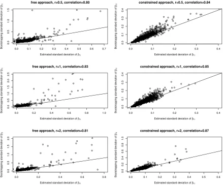
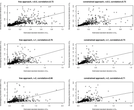
Because the test statistic we use is a Wald statistic, the standard deviation SE( ˆβ1i) of

the estimated parameter ˆβ1i is critical to evaluate the corresponding p-value. Inaccurate SE( ˆβ1i) may lead to incorrect p-values, and misleading type I error or power afterwards.

In order to check the accuracy of SE( ˆβ1i) by our proposed ZIBB method, we compare

it with the one calculated using a bootstrap strategy. For a sufficient sample size, the bootstrap standard deviations are likely to be good estimates of the true standard error.

Using the same data generation strategy as in the simulations above, we are able

to obtain a simulated microbiome count dataset (Y, X, Z) with m OTUs and n

sam-ples. Applying ZIBB method on this dataset, we can calculate corresponding standard

deviations {SE( ˆβ1i)}i=1,...,m for parameter β1i. Then, we construct B = 100 bootstrap

datasets {(Y(b)_{, X}(b)_{, Z}(b)_)}

b=1,...,B. Each bootstrap dataset (Y(b), X(b), Z(b)) is generated

(39)

bootstrap dataset, we calculate the estimated parameter {βˆ₁(b_i)}i=1,...,m. For a specific

OTUi, the standard deviation of estimated ˆβ₁(b_i) across all bootstrap datasets is denoted it as SE( ˆβB

1i). We then compare the standard deviations {SE( ˆβ1i)}i=1,...,m by the ZIBB

method to the standard deviations{SE( ˆβB

1i)}i=1,...,m by bootstrapping.

We check the accuracy of estimated standard deviations by using both the free

model-ing approach and constrained modelmodel-ing approach. For the discrete case (i.e., phenotype

is discrete), the sample size is n1 = 50 versus n2 = 50. For the continuous case, the sample size is n= 100. The number of OTUs is m = 3000. To determine the true value

for β1i, three effect size r values are chosen,r = 0.5,1,2.

2.4.2 Simulation for prediction study

This simulation compared the performances of various methods for predicting missing

phenotypes. In this simulation, the overall settings are similar to the discovery study.

Again, we consider two types of phenotype: discrete and continuous. For both cases, only one phenotype is included. The design matrix X for count model (2.4) is then a

n-by-2 matrix, where n is the number of samples. The first column of X are 1’s which

correspond to intercept. The second column of X are the phenotypes {x1j}j=1,...,n. The

goal is to predict the values for some missing x1j’s.

In this simulation, we divide all OTUs (total number is m) into groups of size 30.

To set the true values for the beta parameters, we first determine β0i using the same

method as in the simulation settings for discovery study (Section 2.4.1). Forβ1i’s, we set

the first parameters of the first two OTU groups to be non-zero (i.e.,β1,1 and β1,31), all other{β1i}i=2,...,30,32,...,m as zeros. Therefore, in this simulation setting, only the first two

groups have true effects. The two none-zero β1,1 and β1,31 are determined by the effect size r as in Section 2.4.1. Here, we choose r= 2.

For the discrete case (phenotype x1j is discrete), the x1j are indicators for the two

groups. The two groups have the same sample size (n1 = 10 versus n2 = 10, n1 = 50 versus n2 = 50). For the continuous case (phenotype x1j is continuous), the x1j are

random samples from a standard normal distribution, and the total sample size is either

n = 20 or n = 100. Once obtaining the true values for beta’s and matrixX, we use the

same data generation procedure as in simulations for the discovery study (Section 2.4.1)

(40)

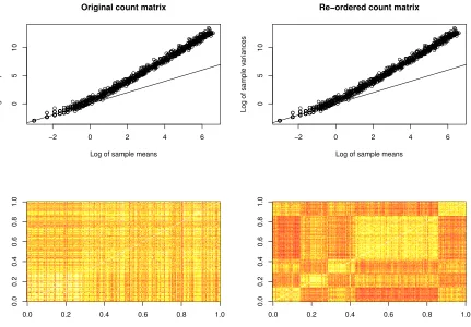
In order to simulate groups of correlated OTUs while maintaining realistic

mean-variance structure, we devised a novel row-ordering strategy for microbiome count data

Y. The approach uses an approximate target within-cluster (rank) correlationρ1 >0 for all pairs of OTUs within each cluster. In addition, the approach can be used to specify

that a cluster has correlationρ2 with a phenotypex. We assume thatxhas been re-scaled to have mean zero, variance 1. Letkdenote a cluster, and Ωkindex the collection of OTUs

in the cluster. For a cluster that is not correlated withx, a “prototype”N(0,1) vectorak

is first simulated. Then, for each OTUi∈Ωk, a new random normal deviate is simulated, Bi =

p

ρ1−ρ22 ak+ρ2x+, where∼N(0,1−ρ21). For two different OTUs i1 and i2 in the cluster, this approach ensures corr(Bi1, Bi2) =ρ1 while corr(Bi1, x) =ρ2. Next, the

count matrix valuesY are re-ordered according to each corresponding realizedbivector to

create a new matrixY0. Specifically, let subscript (j) refer to thejth order statistic, and

rank(bi) be the vector of ranks of bi, with jth element rank(bi)j. Then Yij0 =Yi(rank(bi)j)

for i∈Ωk, j = 1, ..., n. As the Pearson correlation of bivariate normal random variables

is approximately equal to the rank correlation, this approach ensures that the re-ordered

Y0 matrix has elements in each cluster with rank correlation approximating the targets

ρ1, ρ2. In the simulations shown, the correlations ρ1 are held constant for each cluster, while the correlation ρ2 is chosen to be nonzero for only 10% of clusters. We note that the re-ordering procedure does not change the matrix elements ofY, but merely re-orders each row. Thus the mean-variance relationship is preserved. The re-ordered Y0 matrix

will then replace original Y matrix, and be treated as the new simulated microbiome

count values.

LASSO and group LASSO are chosen as the competing methods. To evaluate the

performance of each method, we employ 10-fold cross validation. The whole dataset is

divided into 10 subsets with equal size. Take 9 of the 10 subsets as training data and

the remaining 1 subset as testing data. We computed the mean squared error (MSE)

on the testing data for each competing method. Repeat the above process 10 times to

make sure that each subset will be tested. In order to calibrate the measure of MSE, we also check the correlation between predicted and true values. One-hundred datasets

were generated using the procedures above under each scenario. Each dataset includes