Efficient smile detection by Extreme Learning Machine

UC Riverside

UC Riverside Previously Published Works

Efficient smile detection by Extreme Learning Machine Permalink https://escholarship.org/uc/item/35f876kn Journal NEUROCOMPUTING, 149(Part A) ISSN 0925-2312 Authors An, Le Yang, Songfan Bhanu, Bir Publication Date 2015-02-03 DOI 10.1016/j.neucom.2014.04.072 Peer reviewed

Efficient Smile Detection by Extreme

Learning Machine

Le An

∗

, Songfan Yang and Bir Bhanu

Center for Research in Intelligent Systems, University of California, Riverside, CA 92521, USA

Abstract

Smile detection is a specialized task in facial expression analysis. As one of the most important and informative expressions, smile conveys the underlying emotion status such as joy, happiness, and satisfaction. Smile detection has many applica-tions in practice such as camera photo capture, computer games, monitoring status of patients, etc. Normally smile detection is approached as a binary classification problem. Although many existing classifiers such as Support Vector Machine can perform well for the binary classification task, the required time for training and/or prediction may exceed the requirement for real-time applications. In this paper, an efficient smile detection approach is proposed. The faces are first detected and a holistic flow-based face registration is applied which does not need any manual labeling or key point detection. The Extreme Learning Machine (ELM) is used for training the smile detection classifier and predicting the state of a given face. The proposed smile detector is tested with different feature representations. The proposed approach is validated using not only the faces from controlled databases but also a real-life smile database. The comparisons against benchmark classifiers suggest that the proposed method using ELM is both efficient and effective with different feature descriptors.

Key words: Facial expression analysis, smile detection, Extreme Learning Machine, classification, feature extraction.

1 Introduction

Facial expression analysis plays a significant role in understanding human emo-tions and behaviors. The varying facial expressions are considered the most

∗ _{Corresponding author}

Figure 1. Two AUs (AU 6 and AU 12) that account for smile.

important cues in the psychology of emotion [1]. Analyzing facial expressions accurately has broad applications in areas such as human behavior analy-sis, human-human interaction, and human-computer interaction. Automatic recognition of emotion from images or videos of human facial expression has been a challenging and actively studied problem for the past few decades [2]. Six basic facial expressions and emotions that are commonly referred include anger, surprise, disgust, sadness, happiness and fear. To quantitatively study various facial expressions, facial action coding system (FACS) has been devel-oped [3]. In total 44 Action Units (AUs) are defined to describe all possible and visually detectable facial changes.

Among different facial expressions, happiness, as usually demonstrated in a smile, frequently occurs in a person’s daily life. Smile involves two parts of facial muscle movements, namely Cheek Raiser (AU 6) and Lip Corner Puller (AU 12), as shown in Figure 1. Smile conveys the emotion indicating joy, hap-piness, satisfaction, etc. As a consequence, some research has been dedicated to smile detection [4] [5] [6]. Although accurate smile detection can be achieved in a laboratory controlled database, smile detection for real-life face images is still challenging due to the variations in pose, illumination and image quality. Figure 2 shows some smile and non-smile real-life face images.

In this paper, we focus on detecting smiles from face images that contain either a smile or non-smile facial expression. The discriminative classifier is trained

in an efficient manner using Extreme Learning Machine (ELM) [7]. ELM is a recently proposed learning framework which has very low computational cost without the hassle of parameter tuning in contrast to the other learning methods. ELM has been previously applied to different tasks such as image super-resolution [8], genome analysis [9], human action recognition [10], face recognition [11], face emotion recognition [12], etc. Before training the clas-sifier, we use a standard face detector [13] to detect faces from the images. The faces are registered using a flow-based affine transformation automati-cally without any manual labeling or key-point detection. The trained model by ELM is then used to predict the smile status of a given face. Experiments, on a collection of laboratory controlled database and a real-life database, us-ing various feature representations show that the proposed approach achieves high accuracy and efficiency compared to the benchmark classifiers.

The reminder of this paper is organized as follows. In Section 2 related work is reviewed. The proposed method for smile detection is presented in Section 3. Section 4 is dedicated to the experimental results. Finally, we conclude this paper in Section 5.

2 Related Work

For facial expression recognition, mainly two directions have been explored: geometric-based approaches and appearance-based approaches.

Geometric-based approaches track the facial geometry information over time and infer expressions based on the facial geometry deformation. In [14] a set of points as the facial contour feature is defined, and an Active Shape Model (ASM) is learned in a low dimensional space. In this way the mismatch due to non-linear image variations is avoided. Luceyet al.[15] use Active Appearance Model (AAM)-derived representation for expression recognition together with normalization techniques to improve the recognition performance. A particle filtering scheme is used to track the fiducial facial points in a video for facial expression recognition in [16]. In [17] the geometrical displacement of certain grid nodes on face landmarks placed manually by users is used as input to the multi-class Support Vector Machine (SVM) for facial expression recognition in image sequences.

Appearance-based approaches emphasize on describing the appearance of fa-cial features and their dynamics. Bartlett et al. [18] use a bank of Gabor wavelet filter to decompose the facial texture and the AdaBoost and SVM are used for subsequent classification. In [19] the dynamic texture, which com-bines the motion and appearance along the time axis, is used by extracting the volume of local binary patterns (VLBP). Wu et al. [20] explore Gabor

Motion Energy Filters (GME) as a biologically inspired facial expression rep-resentation. Most recently, Yang et al. [21] propose a new image-based face representation and an associated reference image called Emotion Avatar Image (EAI), which aggregates the dynamics of the facial expression change into a single image. The experiments show that the EAI is a very strong yet compact cue for expression inference.

Apart from abundant literature for facial expression recognition, a few papers are dedicated to smile detection. In [22], smile detection is achieved by using Fisher weight map (FWM) and higher-order local auto-correlation (HLAC). In [6] a real-world image collection of thousands subjects is introduced. Com-prehensive studies are conducted by examining different aspects such as size of database, effect of image registration, image representation and classifier. Re-sults show that human-level expression recognition accuracy can be achieved using current machine learning methods. Recently, Shan [5] proposes using pixel intensity difference as features for smile detection. AdaBoost is used to choose the weak classifiers and a strong classifier is formed by combining the chosen weak classifiers. This approach achieves state-of-the-art results on a real-life smile detection database.

Besides image-based approach, some methods integrate multi-modal informa-tion for smile detecinforma-tion. Itoet al. [23] detect smile using an image-based facial expression recognition combined with an audio-based laughter sound recogni-tion method. In [4] audio features from the spectogram and the video features extracted by estimating the mouth movement are used in stacked sequential learning for smile detection.

For commercial applications, some software tools have been developed for smile detection, such as VDFaceSDK [24] and Omron’s smile measurement and analysis software [25].

3 Technical Approach

The system pipeline of the proposed approach is shown in Figure 3. Before face registration, the faces are extracted from the original images using a standard face detector. The detected faces are registered using a fully automated flow-based registration method without the manual labeling of key points. The facial features are then extracted from the registered faces. The ELM is used to train the smile/non-smile binary classifier and the learned model is used to predict the smile status of a given face for testing. In the following each step will be explained in detail.

Figure 3. The pipeline of the proposed method for smile detection. After faces are detected from the original images, a flow-based face registration is performed to align the faces. Then the features are extracted from the registered faces as input to the ELM. With the learned model, the ELM classifier is able to predict the smile status of a given face.

3.1 Face Detection

The faces from original images are extracted using Viola-Jones face detec-tor [13] implemented in OpenCV which is suitable for real-time processing. The Viola-Jones face detector performs well and the detection accuracy is very high at low false alarm rate. The detected faces are normalized to a certain image size using the bicubic interpolation.

3.2 Face Registration

Face registration/alignment normally requires the knowledge of the facial key points such as the locations of the eyes, nose, and mouth. Facial points lo-calization is either performed through manual labeling or by an automated detector (e.g. [26]). When the image is noisy or of low-resolution, the key points detection is prone to error. In our approach, we apply a holistic flow-based face registration method to automatically align the detected faces. No facial points need to be located in this way and the registration produces the smooth output that is robust to minor out-of-plane head rotations. The face registration involves two steps: SIFT flow computation and flow-based affine transformation.

3.2.1 SIFT Flow Computation

SIFT flow [27] was originally designed for image alignment at the seman-tic level. This higher level alignment is achieved by matching local, salient and transform-invariant image structures. The SIFT flow algorithm robustly matches dense SIFT features between two images, while maintaining spatial discontinuities. The local gradient descriptor, SIFT [28], is used to extract a pixel-wise feature component. For every pixel in an image, its neighborhood (e.g. 16×16) is divided into a 4×4 cell array. The orientation of each cell is quantized into 8 bins, generating a 4×4×8 = 128-dimension vector as the SIFT representation for a pixel, or the so called SIFT image. For face registration, the goal is to register an input face to a reference face with the

desired pose and view.

After obtaining the SIFT descriptors for every pixel in the input face image and the reference face image, a dense correspondence (SIFT flow) is built between these two images. The objective energy function to be minimized is defined as: E(w) =X p min(ks1(p)−s2(p+w(p))k1, t)+ (1) X p η(|u(p)|+|v(p)|)+ (2) X (p,q)∈ε min(α|u(p)−u(q)|, d)+ min(α|v(p)−v(q)|, d) (3)

wherep= (x, y) is the grid coordinates of the images, andw(p) = (u(p), v(p)) is the flow vector at p. u(p), v(p) are the flow vectors for x direction and y direction respectively.s1ands2 are two SIFT images to be matched.εcontains all the spatial neighbors (a four-neighbor system is used). Thedata term in (1) is a SIFT descriptor match constraint that enforces the match along the flow vectorw(p). Thesmall displacement constraint in (2) allows the flow vector to be as small as possible when no other information is available. Thesmoothness constraint in (3) takes care of the similarity of flow vectors for adjacent pixels. In this objective function, the truncatedL1 norm is used in both the data term and the smoothness term with tand d as the thresholds for matching outliers and flow discontinuities, respectively. η and α are scale factors for the small displacement and smoothness constraint, respectively. The dual-layer loopy belief propagation is used as the base algorithm to optimize the objective function. Then, a coarse-to-fine SIFT flow matching scheme is adopted to improve the speed and the matching result.

3.2.2 Flow-based Affine Transformation

After the SIFT flow is computed, instead of detecting key points on the input face (e.g., eye corners, mouth center) and inferring affine transformation from them, we use the SIFT flow information to estimate an affine transformation from the input face image to the reference face. In homogeneous coordinates, we represent the pixel location of a target frame and a reference frame by

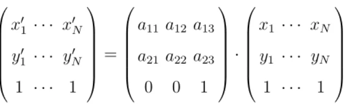
p = (x, y,1) and p0 = (x0, y0,1), respectively. Given the target frame pixel location and its corresponding flow vectors, the reference frame pixel location can be written as x0 =x+u(p),y0 =y+v(p). Thus, we can model the affine transformation for all N pixels in a image as follows:

       x0₁ · · · x0_N y₁0 · · · y_N0 1 · · · 1        =        a11 a12 a13 a21 a22 a23 0 0 1        ·        x1 · · · xN y1 · · · yN 1 · · · 1       

To suppress the outliers from the flow vectors, we solve for the maximum likelihood estimates of this overdetermined system robustly by iteratively reweighted least squares (IRLS) [29].

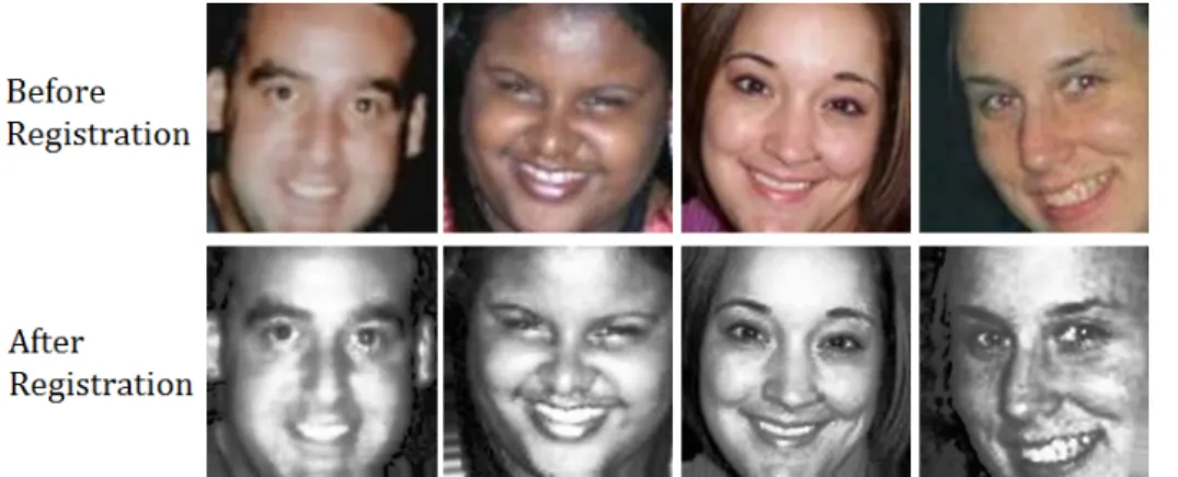
The reference face is obtained by averaging all of the frontal faces in the CK+ database [30]. The SIFT flow based registration from an input face to the reference face is illustrated in Figure 4. Note that the original flow vectors are discontinuous, and the corresponding warping result using the discontinuous flow vectors has strong artifacts. The affine transformation makes the flow vector field continuous and the warping result using the affine transformed flow vector field is smooth without artifacts. Figure 5 shows some sample results of face registration.

Figure 4. SIFT flow based face registration. The SIFT flow is first computed between the input face and the reference face. Affine estimation is used to transform the original discontinuous flow vector filed to a smooth flow vector field. The aligned face using smoothed flow vector field contains much less artifact compared to the aligned face using the original flow vector field.

3.3 Feature Extraction

To extract feature representations for faces, various feature descriptors have been proposed. In the experiments, We adpot three most popular feature

de-Figure 5. Samples of faces before and after registration.

scriptors: Local Binary Pattern (LBP) [31], Local Phase Quantization (LPQ) [32], and Histogram of Oriented Gradients (HOG) [33]. The operation of each fea-ture descriptor is explained in the following sections. In addition, the raw pixel intensity values are also used as a baseline feature descriptor.

3.3.1 LBP

Local Binary Pattern (LBP) [31] and its derivatives are among the most popu-lar choices for facial feature representations. The basic LBP feature for a pixel is obtained by comparing its intensity value to the eight immediate neigh-bors and the generated LBP code is converted to an integer value between 0-255. The LBP descriptor for the whole image is generated by building up the histogram for the LBP code for each pixel. Figure 6 shows the basic LBP operator.

Figure 6. The basic LBP descriptor.

In the experiments, an extended version of uniform and grayscale invariant LBP is used [34], as represented byLBPu2

P,R.u2 denotes the uniform property

and the LBP operator works in a circularly symmetric neighborhood with P pixels on the circle of radiusR. The uniform pattern reduces the 256 possible basic LBP patterns to 59. The image is divided into 10 blocks and in each block a histogram is built by accumulating the occurrence of various patterns. The final feature descriptor for the whole image is obtained by concatenating the histograms from each block.

3.3.2 LPQ

The LPQ descriptor is originally proposed in [32] as a blur insensitive feature representation. The merit of blur insensitivity of LBP comes from the property that the phase of the original image and the blurred image has invariant phase when the point spread function (PSF) is centrally symmetric. At each pixel locationx= [x1,x2]T in a neighborhoodNxof the imagef(x), the local spectra

are computed using a discrete short-time Fourier transform (STFT) by

F(u,x) = X

y

f(y)w(y−x)e−j2πuTy (4)

At each pixel position we obtain a vector

F(x) = [F(u1,x), F(u2,x), F(u3,x), F(u4,x)] (5)

where u1 = [a,0]T, u2 = [0, a]T, u3 = [a, a]T, and u4 = [a,−a]T, where a is a small scalar to ensure that H(u)>0 and w(x) defines the neighborhoodNx.

The local Fourier coefficients are computed at four frequency points and the phase information is recorded by a binary quantizer that observes the signs of the real and imaginary parts of each component in F(x). The resulting binary coefficients are then represented as integer values between 0-255. For each image block, a histogram is generated from the calculated integer values. The final feature descriptor for the entire image is obtained by concatenating all the histograms from different blocks.

3.3.3 HOG

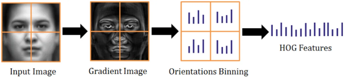
HOG was originally proposed for human detection with success [35]. Recently it has been applied to face recognition [33]. HOG operates by first computing the image gradients in horizontal and vertical directions of an image. The image is then divided into blocks and for each block, the orientation for each pixel is binned into evenly divided orientation channels spreading from 0-180 or 360 degrees. The final descriptor is the concatenations of HOG histograms from each block. Since the HOG is a local-region based descriptor, it tolerates some geometric and photometric variations. Figure 7 illustrates the basic idea of HOG feature computing.

Figure 7. The generation of HOG features.

3.4 ELM for Smile Detection

ELM was initially developed for single-hidden-layer feed-forward neural net-works (SLFNs) [36]. According to ELM theory, the hidden node parameters can be generated before seeing the training data, which is contrary to the conventional learning methods. The output function of ELM is designed as:

fL(x) = L

X

i=1

βihi(x) =h(x)β (6)

whereβ= [β1, β2, ..., βL]T is a vector consisting of the output weights between

the hidden layer and the output node. h(x) = [h1(x), h2(x), ...hL(x)]T is the

output of the hidden layer given input x. Function h(x) maps the original input data space to theL-dimensional feature space.

According to [7], ELM does not only aim at reaching the minimum training error but also the smallest norm of the output weights, which would yield a better generalization performance. Thus, in ELM the following quantities are minimized minimize    kHβ−Tk2 kβk (7)

where T contains the training target value and H is the the hidden-layer output matrix H=        h1(x1) · · · hL(x1) .. . ... h1(xN)· · · hL(xN)        (8)

In the implementation, the minimal norm least square method is used instead of standard optimization method [36]. ELM has several advantages over the

other classifiers: 1. ELM can be applied in both multi-class classification and regression problems with various types of feature mappings; 2. Compared to other classifiers such as Support Vector Machine (SVM), ELM has milder optimization constraints; 3. ELM requires much less computation compared to SVM or Neural Networks (NN); 4. In the training process the hassle of parameter tuning is avoided and the generalization performance of ELM is not sensitive to the number of hidden nodes as tested in [7]. These merits make ELM very efficient and user-friendly in different learning schemes such as batch mode learning and online incremental learning.

The features extracted from both smile and non-smile faces are used as training data. The training data and their corresponding labels (smile and non-smile) are fed to ELM to learn the discriminative binary classifier. We use the basic version of ELM with randomly generated hidden nodes. Sigmoid function is chosen as the activation function. The only parameter to be defined is the number of hidden neurons, which is determined through cross-validation. The training is performed off-line and after training the ELM learning model is saved. For smile detection, features from a given face are extracted and ELM classifier is used to predict its smile status.

4 Experiments

In the experiments two databases are used. One database, referred as the MIX database, is generated as a collection of smile and non-smile images from several publicly available databases. A more challenging database, the GENKI4K database [37] containing real-life smile and non-smile images, is also used for validating the proposed approach. The experimental setup and the results are reported in the following subsections.

4.1 Databases

4.1.1 MIX Database

We collect a set of images called MIX database from four publicly available databases: FEI [38], Multi-PIE [39], CAS-PEAL [40], and CK+ [30]. The FEI database is a Brazilian face database containing images of participants who are between 19 and 40 years old. The Multi-PIE database contains images of 337 subjects with different poses and facial expressions. The CAS-PEAL database is a Chinese face database that involves 1042 subjects. The CK+ database is an extensive database for action unit and emotion specified facial expression. In total we select 1534 smile faces and 2035 non-smile faces from these four

databases to construct the MIX database. The detected faces are normalized to 200×200 and converted to gray-scale images. The diversity of the MIX database is addressed by the wide range of age, ethnicity, imaging condition, occlusions (e.g., glasses), etc. Some sample images from the MIX databases are shown in Figure 8. In the experiments four-fold cross-validation is performed on this database, meaning that each time 75% images are randomly selected as training images and the rest 25% images are used for testing.

Figure 8. Sample images from the MIX database as a collection of images from FEI [38], Multi-PIE [39], CAS-PEAL [40], and CK+ [30] databases. Smile faces (top row) and non-smile faces (bottom row) are shown.

4.1.2 GENKI4K Database

The GENKI4K database [37] contains 4000 face images of a wide range of subjects with different age and race in real-life pictures with varying pose, illumination and imaging conditions. Among these 4000 images, 2162 images are labeled as smile and the rest 1828 images are labeled as non-smile. This database represents the real-life scenarios for smile detection which is more challenging than detecting smiles in laboratory-controlled databases. Figure 9 shows some sample images from the GENKI4K database.

In our experiments the detected faces from the original images are converted to gray-scale images with the size normalized to 100×100. Four-fold cross-validation is performed on this database, meaning that each time 3000 images are randomly selected as training images and the rest 1000 images are used for testing. Table 1 summaries the aforementioned two databases used in the experiments.

Figure 9. Sample images from GENKI4K [37] database. Smile faces (top row) and non-smile faces (bottom row) are shown.

Database Total Size Smile Faces Non-Smile Faces Image Dimension MIX 3569 1534 2035 200×200 GENKI4K [37] 4000 2162 1828 100×100 Table 1

Two databases used in the experiments.

4.2 Parameter Settings

For LBP, LPQ and HOG, the image is divided into 10×10 blocks. In LBP, LBPu2

8,2 is used as suggested in [31] for face representation. The parameters for LPQ are set to M = 7, α = 1/7 and ρ = 0.9. For HOG, the number of orientation bins is set to 15. Besides these three feature descriptors, the raw pixel intensity values are also used as a baseline feature descriptor. The dimensionality of the extracted feature vectors is reduced to 500 using PCA. For ELM, the number of hidden neurons are set to 600 by cross-validation. For SVM, the soft margin parameterC is set to 10 by cross-validation.

4.3 Benchmark Classifiers

The proposed method using ELM is compared with two benchmark classifiers: Linear Discriminant Analysis (LDA) and Support Vector Machine (SVM). These classifiers are commonly used in classification tasks. For the SVM clas-sifier, its linear version is used.

4.4 Detection Performance

The detection accuracy for the MIX and GENKI4K databases are shown in Table 2 and Table 3. Compared to the results by LDA and SVM, ELM achieves better or similar performance. By using different features we observe the same performance trend. LPQ combined with ELM achieves the best detection ac-curacy of 94.6% for the MIX database and HOG+ELM gives the best re-sult of 88.2% for the GENKI4K database. For the MIX database, even with pixel intensity values as features, the detection rates using different classi-fiers are above 90% and using more advanced features brings the detection rate to nearly 95%. The high detection accuracy on the MIX database indi-cates that for the lab-controlled databases, the current framework works very well. For the real-life scenario database, using advanced features help improve the detection rate significantly yet the best accuracy is still lower than the laboratory-controlled database. Both SVM and ELM outperform LDA on the two databases.

Feature → Pixel Values HOG LBP LPQ Classifier↓

LDA 90.8 93.2 92 92.1 SVM 92.9 94.2 93.9 94.3 ELM 93.1 94.4 94.2 94.6

Table 2

Smile detection accuracy for the MIX database (in %).

Feature → Pixel Values HOG LBP LPQ Classifier↓

LDA 74.7 85.7 76.6 78.5 SVM 79.4 87.1 84.2 84.4 ELM 79.3 88.2 85.2 85.2

Table 3

Smile detection accuracy for the GENKI4K database (in %).

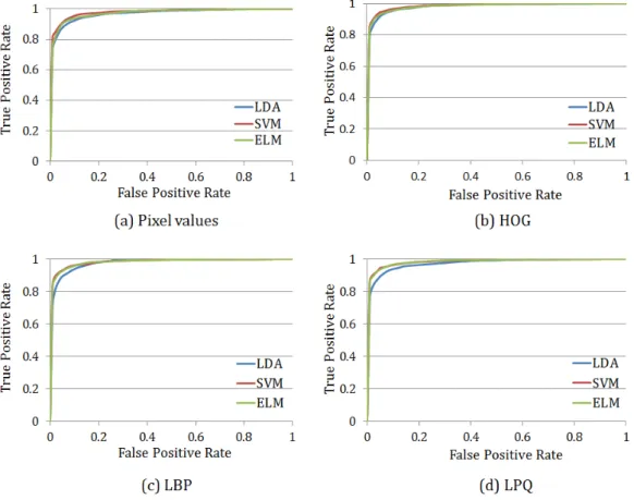
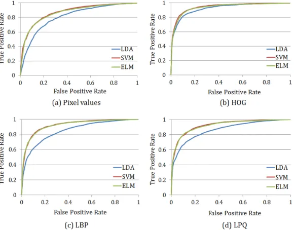
The ROC curves for the MIX and GENKI4K databases with different feature descriptors are shown in Figure 10 and Figure 11. The performance of ELM and SVM is quite similar at different false positive rates and both of them outperforms LDA.

The Area Under Curve (AUC) for the ROC curves in Figure 10 and Figure 11 is given in Table 4 and Table 5. As a performance measure for classifiers, AUC indicates the probability that a classifier will give a higher rank to a randomly chosen positive sample than a randomly chosen negative sample. Although

Figure 10. The ROC curves for the MIX database with different feature descriptors. (a) Pixel values. (b) HOG. (c) LBP. (d) LPQ.

Feature→ Pixel Values HOG LBP LPQ Classifier ↓

LDA 0.961 0.983 0.979 0.976

SVM 0.978 0.987 0.985 0.987

ELM 0.976 0.986 0.985 0.987

Table 4

Area Under Curve (AUC) for the MIX database.

Feature→ Pixel Values HOG LBP LPQ Classifier ↓

LDA 0.815 0.927 0.851 0.866

SVM 0.877 0.947 0.923 0.925

ELM 0.87 0.946 0.921 0.923 Table 5

Figure 11. The ROC curves for the GENKI4K database with different feature de-scriptors. (a) Pixel values. (b) HOG. (c) LBP. (d) LPQ.

overall the AUC for SVM is slightly higher than that of ELM with different feature descriptors, the AUC values for both SVM and ELM are very close. This indicates that as a binary classifier, ELM is very competitive compared to SVM.

Table 6 shows the comparison between the best result by the proposed method and the most recent result on the GENKI4K database [5]. In [5], pixel differ-ence is used as the feature descriptor and AdaBoost is used for feature selection and classification. The experiments in [5] are also carried out with four-fold cross-validation. The detection rate by our method is very close to that in [5]. Note that in [5] the faces need to be manually registered based on eye locations and in our method no manual registration is required. In addition, in [5] the 500 features are selected by AdaBoost algorithm while in our case the stan-dard HOG features are used and the features after PCA dimension reduction are not further refined. For the proposed approach, different feature descrip-tors including pixel difference can be used to further improve the detection performance.

Method Features Dimension Classifier Detection Accuracy Shan [5] Pixel difference 500 ELM 89.7% Proposed HOG 500 AdaBoost 88.2% Table 6

Comparison to the method in [5] on the GENKI4K database.

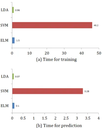
4.5 Computational Cost

The computational cost for the smile detection using ELM is compared against SVM and LDA classifiers. The required times for training and prediction are shown in Figure 12 and Figure 13 for the MIX and GENKI4K databases. The non-optimized codes are implemented in MATLAB on a desktop with 3GHz CPU and 8GB of RAM. For SVM, the LIBSVM1 package is used. Compared to SVM, ELM is significantly faster with time for training and prediction reduced by factor over 30. Note that in this case the ELM is fully implemented in MATLAB and the SVM is implemented in C++ with MATLAB interface. The time cost for LDA is comparable to ELM. However, the performance of LDA is inferior to ELM. The efficiency and accuracy of ELM make the smile detection using ELM reliable and possible for large-scale or real-time practical applications.

4.6 Impact of Number of Hidden Neurons

In the experiments, the only parameter to be determined for ELM is the number of hidden neurons. Figure 14 and Figure 15 shows the detection rates with different number of neurons for the MIX and GENKI4K databases. As can be seen, with a small number of neurons, the detection rate is very low for both databases. The detection rate keeps improving as the number of neurons increases from 100 to 600. Adding more neurons does not help to further boost the performance as the number of neurons goes beyond 600. This supports our choice of 600 neurons for ELM in the experiments.

5 Conclusions

Smile, as one of the most frequent and important facial expressions, conveys emotion for happiness and joy. Smile detection has many potential applica-tions in practice. In this paper, a fully automated smile detection approach using Extreme Learning Machine (ELM) is proposed. The face registration in 1 _{http://www.csie.ntu.edu.tw/ cjlin/libsvm/}

Figure 12. Computational cost for the MIX database. (a) Training time (ins). (b) Prediction time for one face (inms).

our approach is performed automatically in a holistic manner and no manual labeling or key-points detection is required. For the classification, the ELM reduces the computational time significantly compared to the other bench-mark classifiers such as the Support Vector Machine. Experiments on both lab-controlled database and real-life database show that the proposed ELM-based smile detection is very competitive in terms of detection performance with very low computational cost, which enables the potential for real-time applications. The proposed approach is adaptable with any feature descriptors and can be further improved with additional processing steps such as image enhancement and feature selection.

References

[1] J. Russell and J. Fern´andez-Dols,The Psychology of Facial Expression. Studies in Emotion and Social Interaction, Cambridge University Press, 1997.

[2] M. Pantic and L. J. M. Rothkrantz, “Automatic analysis of facial expressions: the state of the art,” IEEE Transactions on Pattern Analysis and Machine Intelligence, vol. 22, no. 12, pp. 1424–1445, 2000.

Figure 13. Computational cost for the GENKI4K database. (a) Training time (in s). (b) Prediction time for one face (in ms).

Figure 14. Detection rate VS number of neurons for the MIX database. [3] P. Ekman and W. Friesen, Facial Action Coding System: A Technique for the

Measurement of Facial Movement. Consulting Psychologists Press, Palo Alto, 1978.

[4] S. Escalera, E. Puertas, P. Radeva, and O. Pujol, “Multi-modal laughter recognition in video conversations,” in IEEE Conference on Computer Vision and Pattern Recognition Workshops, pp. 110–115, 2009.

[5] C. Shan, “Smile detection by boosting pixel differences,” IEEE Transactions on Image Processing, vol. 21, no. 1, pp. 431–436, 2012.

Figure 15. Detection rate VS number of neurons for the GENKI4K database. [6] J. Whitehill, G. Littlewort, I. Fasel, M. Bartlett, and J. Movellan, “Toward

practical smile detection,”IEEE Transactions on Pattern Analysis and Machine Intelligence, vol. 31, no. 11, pp. 2106–2111, 2009.

[7] G.-B. Huang, H. Zhou, X. Ding, and R. Zhang, “Extreme learning machine for regression and multiclass classification,”IEEE Transactions on Systems, Man, and Cybernetics, Part B: Cybernetics, vol. 42, no. 2, pp. 513–529, 2012.

[8] L. An and B. Bhanu, “Image super-resolution by extreme learning machine,” inIEEE International Conference on Image Processing, pp. 2209–2212, 2012.

[9] C. Savojardo, P. Fariselli, and R. Casadio, “Betaware: a machine-learning tool to detect and predict transmembrane beta-barrel proteins in prokaryotes,” Bioinformatics, vol. 29, no. 4, pp. 504–505, 2013.

[10] R. Minhas, A. Mohammed, and Q. Wu, “Incremental learning in human action recognition based on snippets,”IEEE Transactions on Circuits and Systems for Video Technology, vol. 22, no. 11, pp. 1529–1541, 2012.

[11] K. Choi, K.-A. Toh, and H. Byun, “Incremental face recognition for large-scale social network services,” Pattern Recognition, vol. 45, no. 8, pp. 2868–2883, 2012.

[12] A. C. Cruz, B. Bhanu, and N. Thakoor, “Facial emotion recognition with expression energy,” inACM International conference on Multimodal interaction, pp. 457–464, 2012.

[13] P. Viola and M. J. Jones, “Robust real-time face detection,” International Journal on Computer Vision, vol. 57, pp. 137–154, May 2004.

[14] C. Hu, Y. Chang, R. Feris, and M. Turk, “Manifold based analysis of facial expression,” inIEEE Conference on Computer Vision and Pattern Recognition Workshops, pp. 81–81, 2004.

[15] S. Lucey, I. Matthews, C. Hu, Z. Ambadar, F. De La Torre, and J. Cohn, “AAM derived face representations for robust facial action recognition,” in International Conference on Automatic Face and Gesture Recognition, pp. 155– 160, 2006.

[16] M. Valstar, I. Patras, and M. Pantic, “Facial action unit detection using probabilistic actively learned support vector machines on tracked facial point data,” in IEEE Conference on Computer Vision and Pattern Recognition Workshops, pp. 76–76, 2005.

[17] I. Kotsia and I. Pitas, “Facial expression recognition in image sequences using geometric deformation features and support vector machines,” IEEE Transactions on Image Processing, vol. 16, no. 1, pp. 172–187, 2007.

[18] M. Bartlett, G. Littlewort, M. Frank, C. Lainscsek, I. Fasel, and J. Movellan, “Fully automatic facial action recognition in spontaneous behavior,” in International Conference on Automatic Face and Gesture Recognition, pp. 223– 230, 2006.

[19] G. Zhao and M. Pietikainen, “Dynamic texture recognition using local binary patterns with an application to facial expressions,” IEEE Transactions on Pattern Analysis and Machine Intelligence, vol. 29, no. 6, pp. 915–928, 2007.

[20] T. Wu, M. Bartlett, and J. R. Movellan, “Facial expression recognition using Gabor motion energy filters,” in IEEE Conference on Computer Vision and Pattern Recognition Workshops, pp. 42–47, 2010.

[21] S. Yang and B. Bhanu, “Understanding discrete facial expressions in video using an emotion avatar image,” IEEE Transactions on Systems, Man, and Cybernetics, Part B: Cybernetics, vol. 42, no. 4, pp. 980–992, 2012.

[22] Y. Shinohara and N. Otsu, “Facial expression recognition using Fisher weight maps,” in IEEE International Conference on Automatic Face and Gesture Recognition, pp. 499–504, 2004.

[23] A. Ito, X. Wang, M. Suzuki, and S. Makino, “Smile and laughter recognition using speech processing and face recognition from conversation video,” in International Conference on Cyberworlds, pp. 8 pp.–444, 2005.

[24] VDFaceSDK. http://www.visidon.fi/en/Products.

[25] Omron OKAO Vision Smile Measurement and Analysis Software. http://www.omron.com/r d/coretech.

[26] J. M. Saragih, S. Lucey, and J. F. Cohn, “Face alignment through subspace constrained mean-shifts,” in International Conference on Computer Vision, pp. 1034–1041, 2009.

[27] C. Liu, J. Yuen, and A. Torralba, “Sift flow: Dense correspondence across scenes and its applications,” IEEE Transactions on Pattern Analysis and Machine Intelligence, vol. 33, no. 5, pp. 978–994, 2011.

[28] D. G. Lowe, “Distinctive image features from scale-invariant keypoints,” International Journal on Computer Vision, vol. 60, pp. 91–110, Nov. 2004.

[30] P. Lucey, J. Cohn, T. Kanade, J. Saragih, Z. Ambadar, and I. Matthews, “The extended Cohn-Kanade dataset (CK+): A complete dataset for action unit and emotion-specified expression,” in IEEE Computer Society Conference on Computer Vision and Pattern Recognition Workshops, pp. 94–101, 2010.

[31] T. Ahonen, A. Hadid, and M. Pietik¨ainen, “Face recognition with local binary patterns,” inEuropean Conference on Computer Vision, pp. 469–481, 2004.

[32] V. Ojansivu and J. Heikkila, “Blur insensitive texture classification using local phase quantization,” in International Conference on Image and Signal Processing, pp. 236–243, 2008.

[33] O. D`eniz, G. Bueno, J. Salido, and F. D. la Torre, “Face recognition using histograms of oriented gradients,” Pattern Recognition Letters, vol. 32, no. 12, pp. 1598 – 1603, 2011.

[34] T. Ojala, M. Pietikainen, and T. Maenpaa, “Multiresolution gray-scale and rotation invariant texture classification with local binary patterns,” IEEE Transactions on Pattern Analysis and Machine Intelligence, vol. 24, no. 7, pp. 971–987, 2002.

[35] N. Dalal and B. Triggs, “Histograms of oriented gradients for human detection,” in IEEE Conference on Computer Vision and Pattern Recognition, vol. 1, pp. 886–893 vol. 1, 2005.

[36] G.-B. Huang, Q.-Y. Zhu, and C.-K. Siew, “Extreme learning machine: a new learning scheme of feedforward neural networks,” inIEEE International Joint Conference on Neural Networks, vol. 2, pp. 985 – 990 vol.2, July 2004.

[37] The MPLab GENKI Database, GENKI-4K Subset. http://mplab.ucsd.edu.

[38] C. E. Thomaz and G. A. Giraldi, “A new ranking method for principal components analysis and its application to face image analysis,” Image and Vision Computing, vol. 28, no. 6, pp. 902 – 913, 2010.

[39] R. Gross, I. Matthews, J. Cohn, T. Kanade, and S. Baker, “Multi-PIE,”Image and Vision Computing, vol. 28, no. 5, pp. 807 – 813, 2010.

[40] W. Gao, B. Cao, S. Shan, X. Chen, D. Zhou, X. Zhang, and D. Zhao, “The CAS-PEAL large-scale chinese face database and baseline evaluations,” IEEE Transactions on Systems, Man and Cybernetics, Part A: Systems and Humans, vol. 38, no. 1, pp. 149 –161, 2008.