A FPGA pairing implementation using the Residue Number
System
Sylvain Duquesne, Nicolas Guillermin
IRMAR, UMR CNRS 6625 Universit´e Rennes 1 Campus de Beaulieu 35042 Rennes cedex, France
[email protected], [email protected]
Abstract. Recently, a lot of progresses have been made in software implementations of pairings at the 128-bit security level in large characteristic. In this work, we obtain analogous progresses for hardware implementations. For this, we use the RNS representation of numbers which is especially well suited for pairing computation in a hardware context. A FPGA implementation is proposed, based on an adaptation of Guillermin’s architecture which computes a pairing in 1.07 ms. It is 2 times faster than all previous hardware implementations (including ASIC and small characteristic implementations) and almost as fast as best software implementations.
Keywords:Elliptic curves, optimal pairing, Barreto-Naerigh curves, Residue Number System (RNS), efficient hardware implementation.
1
Introduction
2
Pairing on elliptic curves and their computation
Pairings on elliptic curves are bilinear maps from the curve to the multiplicative group of a finite field Fpk wherekis called the embedding degree. It is usually very large so that computing inFpk is
not reasonable. This is reassuring regarding the destructive use of pairings but annoying for pairing based cryptosystems. Small embedding degrees can be easily obtained by using supersingular curves. However, it is too small (k ≤2) if large characteristic base fields are used as in this work. Thus, we use ordinary curves with prescribed embedding degrees constructed via the complex multiplication method as surveyed in [15]. We focused on the most popular one to date, namely the Barreto-Naehrig curves having embedding degree equal to 12 [7]. The reason of their popularity it that ifpis a 256-bit prime number, such curves ensure a 128-bit security level both on the curve and on the finite field
Fp12, assuming NIST recommendations [27].
2.1 Pairings on Barreto-Naehrig curves
Letu∈Z,p= 36u4+ 36u3+ 24u2+ 6u+ 1 a prime number andE an elliptic curve defined overFp
by an equation
y2=x3+a6, (1)
such thatE has prime cardinality`= 36u4+ 36u3+ 18u2+ 6u+ 1. Such curves were introduced in [7]
and have 12 as an embedding degree. This means that`dividesp12−1 but notpk−1 for 0≤k <12
and that the full `-torsion of the curve is defined on the fieldFp12.
Letmbe an integer andQa point onE. If Qm denotes the pointmQ, f(m,Q) is the function on
the curve whose divisor is
div(f(m,Q)) =m Q−Qm−(m−1)O.
This function is the core of all known pairings and is computed thanks to an adaptation of classical scalar multiplication algorithm [25]. In this algorithmg(A,B)is the equation of the line passing through
Algorithm 1: Miller(m, Q, P)
Data: m∈Zwith binary representation (ms−1,· · ·, m0)2,P andQinE(Fp12).
Result:f(m,Q)(P)∈Fp12.
begin
f←1 andT ←Q
fori froms−2downto 0 do f←f2.g(T ,T)(P)
v2T(P) andT ←2T if mi= 1then
f←f.g(T ,Q)(P)
vT+Q(P) andT←T+Q end if
end for returnf end
byA, so that g(A,B)
vA+B is the function onE involved in the addition ofAandB.
In this paper, we are interested in the optimal Ate pairing [26] because it is the most efficient to date for BN curves but the same work can be easily done with other pairings. Ifr= 6u+ 2, it is given by
eo:E(Fp12)∩Ker(π−p)×E(Fp)[`] → F∗p12/ F∗p12
`
(Q, P) 7→ f(r,Q)(P).g(rQ,π(Q))(P).g(rQ+π(Q),−π2(Q)(P)
p
12−1
`
whereπis the Frobenius map on the curve (π: (x, y)7→(xp, yp)).
2.2 Efficient implementation of pairings
An other advantage of BN curves is their degree 6 twist. This means E is isomorphic overFp12 to a curve ˜E defined byy2=x3+a6
ν , whereν is an element inFp2 which is not a cube nor a square. Then we can defined twisted versions of pairings on ˜E(Fp2)×E(Fp)[`]. This means that the coordinates ofQ can be written as (xQν
1
3, yQν12) wherexQandyQ are inFp2. There are three important consequences on the Miller loop.
– Computingg, v,2T andT+Qrequires onlyFp2 arithmetic (but the result remains inFp12).
– The denominators (v2T andvT+Q), and more generally all the factors offlying in a proper subfield
of Fp12, are wiped out by the final exponentiation. This is the famous denominator elimination introduced in [6].
– The numerators (gT ,T andgT ,Q) have the particular formg0+g2ν
1 2 +g3ν
1
3 wheregi∈Fp2 which contains only 6 coefficients instead of 12. Hence the multiplication by such an element during the writing up off is cheaper than a complete multiplication inFp12.
Finally, Koblitz and Menezes show in [23] that the cost of the final exponentiation can be reduced thanks to the integer factorization
p12−1
` = p
6−1
p2+ 1
p4−p2+ 1
`
Then the final exponentiation can be split in two steps
– Powering to thep6−1 and to thep2+ 1. This is easily obtained via cheap Frobenius computations
and an inversion.
– Powering to the p4−p`2+1 which is called the hard part of the final exponentiation. As explained in [17], there are efficient ways to compute it for BN curves and the cost is around three-quarters of the cost of an exponentiation with an exponent having the same size than p. Moreover, as f
has been raised to the p6−1
p2+ 1
, it has orderp4−p2+ 1. Then, as noticed in [17], it is in
GΦ6(Fp2) and squaring such an element (which is the most used operation in the hard part of the exponentiation) is less expensive than a classical squaring inFp12.
As noticed in [12], choosing a RNS based architecture would be of great interest for hardware implementation of pairings. This is due to the massive use of lazy reduction in extension fields. Let us now recall this system for representing numbers and describe our architecture.
3
RNS
3.1 Notation
3.2 Introduction to Residue Number System
LetB ={m1,· · · , mn}be a set of co-prime natural integers, andM = Qn
i=1mi. Let 0≤X < M. The
residue number system (RNS) representation {X}B is the set of positive integers {x1,· · · , xn} with
xi=|X|mi.{x1,· · ·, xn} are called the RNS digits ofX. They are unique for each X, and X can be
recomputed from them using the following fomula :
X =
n X
i=1
|xi×Mi−1|mi×Mi M
whereMi=
M mi
. (2)
The strongest advantage of a such system is that it distributes large integer operations on the small residue values. The operations are performed independently on the residues. In particular, there is no carry propagation over addition, and multiplication complexity is linear withn.M is called the module ofB.
3.3 RNS Montgomery reduction algorithm :
Using RNS representation in B ensures very efficient computation inZ/MZ. To efficiently compute
pairing overFp we need to introduce a reduction bypalgorithm.
The papers [5, 22] propose an adaptation of the well known Montgomery algorithm in the context of RNS representation. We refer the reader to these papers for more details on RNS reduction algorithm. Here we recall the useful results for pairing computation.
We defineB and ˜B two RNS bases of the same sizen, with their coprime modulesM and ˜M. We choose B and ˜B such that M > αpand ˜M >3p(αbeing a parameter defining the maximal value we are able to reduce thanks to this algorithm. See section 5 for the definition in our specific case). For all input A < αp2 given in B and ˜B, the RNS Montgomery algorithm computes S in B and ˜B
such thatS <3pand|S|p=|a×M−1|p. This algorithm calls 2 times theBext(X, B1, B2) subroutine
which computes{|X|M1}B2 from{X}B1.
Algorithm 2: Red(X, p, B,B˜)
Data: Band ˜B RNS bases with moduleM > αpand ˜M >3p, pco-prime withM and ˜M,
{X}B and{X}B˜ RNS representation ofX < αp
2 inB and ˜B,
precalculations :{| −p−1|M}B,{|M−1|M˜}B˜ and{p}B˜,
algorithmBext(A, B1, B2) computing{|A|M2}B2 from{A}B1
Result: {S}B and{S}B˜ such that|S|p=|XM−1|pandS <3p
begin
1 Q←X× | −p−1|M inB
2 Q˜←Bext(Q, B,B)˜
3 R˜←X+ ˜Q×pin ˜B
4 S˜←R˜×M−1
in ˜B
5 S←Bext(S,B, B)˜
There are many ways to realize theBext algorithm. The asymptotically cheapest way being given
in [4] with the overall complexity 75n2+85n RNS digit-products. Nevertheless this version is hardly parallelizable and gives poor results while using it for cryptographic size over a hardware design.
We therefore will use the version of Kawamuraet al. [22]. This algorithm has overall complexity of 2n2+ 3n, but at each time every calculation can be made onnRNS digits in a row.
3.4 The Cox-Rower architecture
The Cox-Rower architecture was first proposed by Kawamura et al. in [22], for the purpose of RSA multiplication. It was enhanced by Guillermin in [18], with support of full arithmetic operations inFp,
and fast elliptic curve scalar multiplication. The main feature of Guillermin’s design is the use of n
parallel Rower achieving one RNS digit multiplication and accumulation per cycle.Band ˜Bare chosen such that∀m∈ {B,B˜}, 2w(1−2−w
2)< m≤2w wherewis the architecture word size, typically 18 or 36 on a FPGA (which embeds very efficient 18×18 multipliers).nis chosen such that 2wn> p. Each
Rower is able to compute at every clock cycle|a×b|mi or|a×b|m˜i. It can also add it simultaneously
with the previous result. The entire design can therefore execute a full length multiplication in 2 cycles (one cycle over B and one over ˜B), an addition in 4 (using 2 accumulated multiplications by 1), a subtraction in 6 (an addition with a multiple of p to keep the result positive is mandatory) and a whole reduction in 2n+ 3 cycles.
An adaptation of Guillermin’s architecture is necessary to provide pairing support. As the number of local variables and precalculations is much larger for pairing computation than for simple elliptic curve scalar multiplication, we used a single triple port RAM of 256 words instead of the ROM and the bunch of 16 registers to store precalculations and temporary results.
These RAMs are generated with the Altera Megawizard tool, and consume only 2 M9k on Stratix III per Rower. Our design for 256-bit curves only requires 8% of the EP3SE50F484, the smallest FPGA of the Stratix III series. We made this choice for the sake of simplicity, but it can be improved at the price of classical register allocation techniques (for ASIC implementations, among other).
On figure 3 in appendix we present the adaptation of Guillermin’s architecture for pairing compu-tation (with FPGA triple port RAM).
3.5 Finite field arithmetic
The most consuming operation in RNS is the reduction, while multiplication and addition over Fp
have a the same weak complexity. This leads to completely different choices compared to classical multiprecision representation.
Lazy reduction : Let us consider anyE =Pli=0AiBi withAi, Bi∈Fp. We call lazy reduction the
fact that this kind of expression only needs one reduction after the l multiplications. Whereas lazy reduction can be used with classical multiprecision representation, as in [3], it is even more interesting in RNS. Indeed the complexity of the arithmetic is concentrated on the reduction step. For example, a Cox Rower withnRowers (nbeing the size of the RNS basesBand ˜B) needs 2lcycles to compute the unreduced representation ofE (lcycles overB and lover ˜B), and eventually 2n+ 3 cycles to reduce it. The only thing we need to take notice of is theαparameter :M must be up to max(E)/pwithE
positive, unless the result of theRedalgorithm is wrong. We observe that the most consuming part of pairings are multiplications and squaring in extension fields ofFp. If the field extension representations
Extension field optimizations : For considered field extensions (k≤12), reductions are the most consuming part. Nevertheless extension field optimizations may accelerate the overall pairing. In [12], the author studied the complexities of both a RNS and a classical implementation of pairings assuming that interpolation methods are used, such as Karatsuba or Toom-Cook. It spares a multiplication compared to schoolbook at the price of 4 additions or subtractions. These techniques are only useful when the relative cost of a multiplication is high compared to addition. In RNS multiplication has a comparable price with addition, interpolation is therefore less attractive. We do not define in this work any method to find the best way to implement tower field arithmetic for BN curves, but propose specific optimisations for our chosen curves in section 4.1. We justify our choice in section 5.
4
Optimal pairing for BN curves
4.1 Choice of the curve
It is explain in [28] how to generate BN curves having nice properties. For this work we chose two curves both witha6= 2. The first one, calledBN126is defined byu=−(262+ 255+ 1) and has already
been used in [28, 3]. It ensures only 126 bits of security but allows to use lazy reduction techniques without requiring an extra word in 32 or 64-bit architecture. Thanks to the size of the FPGA DSP blocks (18×18), the architecture proposed here can havewup to 36 bits words so that we do not have this restriction and we can consider a curve, calledBN128 really ensuring 128 bits of security without
artificial extra cost. In both cases, our architecture requires n= 8 Rower and the word sizew= 34 ensure sufficient margin for lazy reductions considering the algorithmic choices we made (see section 5 for details). This curve is defined byu=−(263+ 222+ 218+ 27+ 1). In both cases,
Fp12 is defined by the following tower of extensions
Fp2 =Fp[X]/(X2+ 1) =Fp[i]
Fp6 =Fp2[Y]/(Y3−(1 +i)) =Fp2[β]
Fp12 =Fp6[Z]/(Z2−β) =Fp6[γ] (=Fp2[γ]).
This tower of extensions has many advantages, the most important being an efficient multiplication algorithm for the canonical polynomial base. The major difficulty is the apparition of the term 1 +ifor the definition ofFp6. We used then some adaptations of the Guillermin’s architecture [18]. We refer the reader to the section 5 for more details. The optimal Ate pairing on these curves can then be computed thanks to the algorithm 3 wheredbl, addandhard-partare given in appendix. Note that the line 4 is due tou <0 and is potentially expensive (inversion) but thanks to the final exponentiation,f−1can
be replaced byfp6 [3] which is almost for free (conjugation). Moreover, sincer= 6u+ 2 has Hamming
weight 5 (resp. 9) forBN126(resp.BN128),addis used only 6 (resp. 10) times.
4.2 Formulas for Miller loop
Jacobian coordinates are usually used for pairing computations [8, 19, 26] but projective coordinates are more interesting in our case [3, 11]. LetP = (xP, yP)∈E(Fp) andQ∈E(Fp12). Using the degree 6 twist on the curve, Qcan be written (xQγ2, yQγ3) with xQ andyQ ∈Fp2. The ”doubling” step of the Miller loop for optimal pairing is consisting in two stages:
Algorithm 3:optimal(P, Q)
Data:r=|6u+ 2|,P = (xP, yP)∈E(Fp)[`],
Q= (xQγ2, yQγ3)∈E(Fp12)∩Ker(π−p) withxQandyQ∈Fp2.
Result:eo(P, Q)∈Fp12.
begin
1 T = (XTγ2, YTγ3, ZT)←(xQγ2, yQγ3,1) andf←1
fori fromblog2(r)c −2downto 0 do 2 T, g←dbl(T, P) andf ←f2.g
if mi= 1 then
3 T, g←add(T, Q, P) andf←f.g end if
end for
4 T ← −T,f←f−1
5 Q1←π(Q)
6 T, g←add(T, Q1, P) andf←f.g 7 Q2← −π(Q1)
8 T, g←add(T, Q2, P) andf←f.g
9 f←
fp6−1p
2+1
10 f←hard-part(f,|u|).
11 returnf end
.
– The evaluation in P of the tangent line in T to the curve. As recalled in Section 2.2, we do not need to take into account the multiplicative factors lying in a proper subfield of Fpk (they are
cancelled by the final exponentiation).
It is given by algorithm 4 in appendix. The classical formulae are rearranged to highlight the reductions (every temporary results need a reduction exceptF, G, H andt3), and the inherent parallelism in the
local variables (Each line can be implemented in a random order). This is important for avoiding idle state in Cox-Rower (see section 5 for more details). The total cost of this step is 4 multiplications, 5 squaring, 8 reductions inFp2 and 2 modular multiplications of an element ofFp2 by an element ofFp.
Note that multiplications like 2XTYT can be transformed into squaring but at the cost of some extra
additions [3, 11] so that it is not interesting for our design.
In the same way, the addition step is consisting in the sum of T andQfollowed by the evaluation inP of the line passing throughT andQand is given by algorithm 5. The total cost of this step is 11 multiplications, 2 squaring, 10 reductions inFp2 and 2 modular multiplications of an element of Fp2 by an element ofFp.
4.3 Final exponentiation
The line 9 requires a conjugation, an inversion inFp12, a Frobenius computation and a multiplication inFp12. In this ”easy” part of the final exponentiation, the inversion is in fact very expensive. It can be done with only one inversion, 97 multiplications and 35 reductions inFp [12, 19], but the remaining
inversion inFp is done via an exponentiation to thep−2 on our design. For this operation, we use
but presents more independence between the local variables. Due to pipeline idle steps, this operation only needs blog(p)−1cmultiplications for the calculation of X2i (with X the value to inverse), the other operations are executed during the necessary pipeline idle states. Then, there is no need to find more efficient ways to execute the exponentiation here. Hence this step will be very expensive compared to the others or compared to a software implementation. On the contrary, the Frobenius only costs 5 multiplications inFp2and 10 reductions, thanks to the definition of the tower of extensions.
To date, the fastest way for computing the hard part (line 10 of algorithm 3) of the final expo-nentiation involved a multi-addition chain [29]. The corresponding algorithm hard-part is given in Appendix in a way using less temporary variables than in [29]. Moreover, as noticed in [17], f is in
GΦ6(Fp2) and squaring such an element is less expensive than a classical squaring in Fp12. In our context, ifa=P5i=0aiγi withai∈Fp2, the coefficient ofA=a2are given by
A0= 3a20+ 3(1 +i)a23−2a0 A1= 6(1 +i)a2a5+ 2a1
A2= 3a21+ 3(1 +i)a24−2a2 A3= 6a0a3+ 2a3
A4= 3a22+ 3(1 +i)a25−2a4 A5= 6a1a4+ 2a5
More recently, Karabina introduced a compressed form for elements inFp12 which requires less opera-tions to be squared [3, 21]. Unfortunately, this method involves extra inversions so that it is unsuited for our design.
5
Pipeline architecture and extension field arithmetic
In this section we start from the definition of Guillermin’s pipeline [18], and show how to construct efficient hardware for the chosen curve in 4.1. Subsection 5.1 describes constraints we followed during the pipeline architecture process. In subsection 5.2 and 5.3, we justify these optimizations regarding operations in pairing and evaluate their cost in Stratix II ALM. Eventually in subsection 5.4, we evaluate the overall gain in clock cycle brought by these optimizations. Figure 1 recalls the one used by [18] and compares it to ours.
5.1 Pipeline depth
Our goal is to keep the maximal frequency already available in [18]. Additive hardware must be carefully introduced, to keep the critical path under control. On the other hand, we can easily raise the pipeline depth without a lot of cycle loss. Indeed pairing computation provides less dependency between local variables than classical elliptic curve scalar multiplication over Fp. We can use this
parallelism to avoid idle states due to the pipeline effect. Algorithm dbland addshow this inherent parallelism during the Miller loop. On each line, every value are independent with one another. The order in the line is then not important. Operations inFp12 also present such inherent parallelism.
Ifπdis the pipeline depth, a result of an operation is availableπd+ 1 cycles after the computation
began, and soπd independent instructions must be inserted before reusing the result. In [22],πd= 2,
while in [18], πd = 5. During our implementation we found thatπd could be up to 8 and still avoid
idle states in the whole pairing, except forFp inversion (see subsection 4.3).
5.2 Additive hardware for multiplication and squaring inFp2
Using Guillermin architecture, a Fp2 multiplication over the chosen extension costs 12 cycles using naive schoolbook multiplication. Among them, 4 cycles are lost to compute the subtraction due to
i2 =−1. If we add the ability to get the opposite of the result before accumulating it in a pipeline
stage, we spare 4 cycles for every computation. Asi1andi2 are in fact less than 3p(they are reduced
values), the opposite hardware module computes |9p2−x|
mi from xthe output of the pipeline (the
result of the operation needs to remain positive). This module only costs 55 ALM per Rower, and has a critical path suitable with the rest of the design.
Karatsuba optimization for Fp2/Fp is here not efficient. Using Guillermin’s pipeline, no less than
18 cycles is needed. The cost of an adder is around 42 ALM. No way has been found to add hardware to make multiplication fall under 8 cycles while preserving correct pipeline depth and critical path.
The opposite hardware module also spares 4 cycles perFp2 squaring. Another important optimiza-tion for squaring is the capacity to compute|2i1×i2|miin one cycle. Squaring inFp2 falls from 8 cycles
to 6. This optimization only costs 2 muxes per Rower (see figure 1). A side effect of this optimization is the need of the precomputed value 18p2 instead of 9p2 in the opposite module.
5.3 Squaring and Multiplication overFp12/Fp2 :
Schoolbook multiplication and squaring : Let A= {a1,· · · , a12}, B ={b1,· · · , b12} and C =
AB∈Fp12. To optimize schoolbook multiplication and squaring with a Cox-Rower, we aim to execute only oncei1=aiandi2=bj, for all{i, j} ∈ {1,· · ·,12}2. Asi2=−1 andγ6= (1+i), the result|ai×bj|
is either added or subtracted on at most two components ofC. Two selectable accumulators combined with opposite calculations are then of great interest. These hardware modules (a combination of an opposite module and an accumulator) cost 150 ALM per Rower. 4 different types of multiplications and squaring are needed during pairing (cycle counts are given excluding the reduction step, which is exactly the same).
– Squaring in the doubling part of the Miller loop : using schoolbook squaring together with the proposed extra hardware costs 156 cycles. In Guillermin’s pipeline, the same operation is computed in 210 cycles.
– Multiplication by the line in the Miller loop : half the values ofB are equal to 0. Using our extra hardware, this costs 144 cycles instead of 177 cycles.
– Squaring inGΦ6(Fp2). We use the formulae of subsection 4.3. With our extra hardware, we need 84 cycles instead of 160.
– Whole multiplications in the final exponentiation : no specific optimization is proposed. We spend here 288 cycles instead of 382 in Guillermin’s architecture.
Interpolation techniques : As interpolation needs a lot of additions, it may be interesting to put an addition capability in our pipeline. But we need to evaluate if they are useful. We start from Karatsuba for arithmetic inFp12 overFp6, which is the best case for these techniques (interpolation at other levels
Fp12/Fp4,Fp6/Fp2 orFp4/Fp2 would give poorer results). Once again we consider 4 cases seen above :
– multiplication of f by the lineg at line 2 and 3 of algorithm 3 (g having half its term set to 0): the schoolbook multiplication costs 144 cycles, with no need of addition while Karatsuba costs 180 cycles with additional hardware.
– squaring in the miller loop : the schoolbook squaring costs 156 cycles, but could be replaced through : (A+γB)2= (A+B)(A+γ2B)−(1 +γ2)AB
– squaring in the cyclotomic subgroup : here we use algorithm of subsection 4.3. The total cost of it is 84 cycles not considering the reduction step. Karatsuba is not of any help here.
– general multiplication in Fp12. Here Karatsuba could be of some help, replacing the 288 cycles schoolbook multiplication by 264 cycles if we can use an additive instruction (there are 48 such addition instructions, an addition hardware module is then mandatory to make Karatsuba effi-cient). Nevertheless only 20 such general multiplications are needed for pairing overBN126, and
only 26 forBN128 , leading to a spare of respectively 480 and 624 cycles (less than 0.4% of the
total number of instruction).
Finally, adding an addition module to our architecture for interpolation techniques seems to be glob-ally not interesting. Moreover the addition has to be integrated in the pipeline by using muxes and additional registers, and may degrade the maximal frequency. We decided not to implement it.
5.4 final pipeline and cycle spare count
The optimized pipeline definition is given in figure 1. It compares it with original Guillermin’s pipeline. Our different proposed optimizations allows us to spare 25500 cycles for a whole pairing (∼15%). A schematic is given in appendix (figure 7). The final pipeline depth πd is 8. Because of our chosen
arithmetic, the value α defined in subsection 3.2 reaches 378. The worst case is reached during the schoolbook multiplication. Therefore the word lengthwis set to 34 in the Cox-Rower.
Fig. 1.Pipeline description and comparison with [18]
Guillermin [18] Ours
stage 1 M SB1||LSB1=i1×i2 M SB1||LSB1 =i1×i2
stage 2 M SB2||LSB2=M SB1×i (M SB1||LSB1=i1×i2
and (SR2 =|LSB1 + 0|mi and (SR2 =|LSB1 + 0|mi orSR2 =|LSB1 +ROMcox|mi) orSR2 =|LSB1 +ROMcox|mi))
or (M SB2||LSB2=M SB1×2i
andSR2 =|LSB1 +LSB1|mi) stage 3 LSB3 =M SB2×i LSB3 =M SB2×i
andSR3 =|LSB2 +SR2|mi andSR3 =|LSB2 +SR2|mi stage 4 (acc1=|acc1+LSB3|mi SR4 =|SR3 +LSB3|mi
oracc1=LSB3)
and (acc2 =|acc2+SR3|mi oracc1=SR3)
stage 5 o=|acc1+acc2|mi (SR51=|18p
2−
SR4|mi orSR51=SR4)
and (SR52=|18p2−SR4|mi orSR52=SR4)
stage 6 (acc1=|acc1+SR51|mi
oracc1=SR51)
and (acc2=|acc2−SR52|mi oracc22=SR52)
6
Results and comparison
In this section we give our results and compare it to the state of art designs and software implemen-tations.
6.1 Intermediary operations cycle count
At this point the fastest known hardware implementation of pairing on BN curves is given by Fan
et al. in [14]. In this paper they used the Hybrid Modular Multiplication technique to improve Fp
arithmetic, and compute a full R-Ate pairing over a BN curve of security level 128. This work divides the number of necessary cycles to compute a full pairing by a factor of around 3. Here we give the operation details for curvesBN126 andBN128. f2 stands for squaring in Fp12 in the doubling part of the Miller loop, andf.g stands for the line multiplication (including the reduction step).
Op dbl add f2 f.g Miller fpk`−1 e O
[14] 996 1260 1541 1239 311418 281558 592976
BN126507 581 384 372 86530 89581 176111
BN128507 581 384 372 92480 94101 192502
We see that we spare cycles at each step of the calculation, mostly thanks to RNS. Other implemen-tation also exist, but we cannot compare their cycle count with us since they use small characteristic [13, 2] or high speed processors ([3, 8, 26]).
6.2 Overall results and comparison
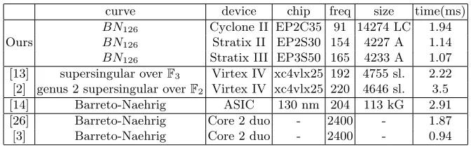
We synthesized our design on 3 target technologies : Altera Cyclone III, Stratix II and Stratix III. The first one, the EP2C35, is a low cost FPGA used for bigger series. Its public price is less than $100 for 1 chip on [1], for the one we used. The second one is proposed for a comparison point with [13, 2] which used a comparable technology with same technological node (Xilinx Virtex IV). We point out the fact that size comparison is not fair, since we do not take in account DSP blocks, and they use none. Our DSP block consumption is important (2 36×36 DSP blocks and 1 9×9 per Rower) and force us to use the second smallest size Stratix II device (the EP2S30). For the Stratix III generation (65nm node), Altera has made a substantial effort to increase the number of DSP blocks. This lets us synthesize the design in the smallest Stratix III of the series (the EPS3SE50). Other point of comparison are given in array 2, for high speed implementations targeting 128-bit security, but on other technologies : ASIC [14], andx86 CPU [26, 3]. We only give the results forBN126. Results forBN128can be deduced
from it, since hardware remains the same (only precomputed values and microcode in the sequencer change).
6.3 Beyond 128 bits
Fig. 2.Overall results and comparison
curve device chip freq size time(ms)
BN126 Cyclone II EP2C35 91 14274 LC 1.94
Ours BN126 Stratix II EP2S30 154 4227 A 1.14
BN126 Stratix III EP3S50 165 4233 A 1.07
[13] supersingular overF3 Virtex IV xc4vlx25 192 4755 sl. 2.22
[2] genus 2 supersingular overF2 Virtex IV xc4vlx25 220 4646 sl. 3.5
[14] Barreto-Naehrig ASIC 130 nm 204 113 kG 2.91
[26] Barreto-Naehrig Core 2 duo - 2400 - 1.87
[3] Barreto-Naehrig Core 2 duo - 2400 - 0.94
use too large curves). We propose here one curve, namedBN192, whoseFp12 relying tower field is con-structed the same way asBN126orBN128. Its parametrization is given byu=−(2160+ 274+ 212+ 1).
Here are the implementation results :
curve FPGA Rowers area cycle count time
BN192EP3SE50 19 9910 ALM 790010 6.02 ms
7
Conclusion
Appendix
Algorithm 4:dbl, doubling step
Data:T = (XTγ2, YTγ3, ZT)∈E(Fp12) withXT, YT andZT ∈Fp2,P = (xP, yP)∈E(Fp). Result: The point 2T and the evaluation inP of the equation of the tangent line inT to the
curve up to multiplicative factors inFp2.
begin
1 B=YT2, C= 3ZT2, D= 2XTYT
2 F =iB−3C, G=iB+3C, H = 3C, t3=B+4iC, A=XT2, E= 2YTZY
3 X2T =DF, Y2T =−iG2+ 2HC, Z2T = 4BE, t0=F yP, t1=−3AxP
4 return(X2Tγ2, Y2Tγ3, Z2T), t0+t1γ+t3γ3
end
Algorithm 5:add, addition step
Data:T = (XTγ2, YTγ3, ZT)∈E(Fp12) withXT, YT andZT ∈Fp2, Q= (xQγ2, yQγ3)∈E(Fp12),P = (xP, yP)∈E(Fp).
Result: The pointT+Qand the evaluation inP of the equation of the line passing throughT
andQup to multiplicative factors inFp2.
begin
1 E=xQZT −XT, F =yQZT −YT
2 E2=E2, F2=F2
3 A=F2ZT −2XTE2−EE2, B=XTE2, E3=EE2
4 XT+Q =AE, ZT+Q =ZTE3, t3=F xQ−EyQ
5 YT+Q=F(B−XT+Q)−yQE3, t0=EyP, t1=−F xP
6 return(XT+Qγ2, YT+Qγ3, ZT+Q), t0+t1γ+t3γ3 end
Algorithm 6:hard-part, hard part of the final exponentiation according [29]
Data:f ∈Fp12 of orderp4−p2+ 1 ,x=|u|
Result:f(p4−p2+1)/`with pand`as in 2.1. begin
computation of theyi
1 y0←fpfp
2 fp3,y
1←fx,y3←y1x,y5←y3x,y4←yp5,y6←y4y5
=fx3fx3p
2 y5←yp3,y2←y5−1,y4←y1y2
=fx/fx2p
3 y2←yp5
=fx2p
2
, y5←y3−1
= 1/fx2,y 3←y
p 1((mx)
p
),y1←f−1
multi-addition chain for computingy0.y12.y26.y123 .y418.y530.y366
4 t0←y26,t0←t0y4,t0←t0y5, t1←y3y5,t1←t1t0,t0←t0y2,t1←t21
5 t1←t1t0,t1←t21, t0←t1y1,t1←t1y0,t0←t20,t0←t0t1 returnt0
Fig. 3.General architecture of a Cox Rower with the triple port RAM
cox cox
main bus
ALU
main bus
sequencer
Triple port RAM
out
cox row1 row2
sequencer
command
in
out
main bus
rown
Fig. 4.design of the pipeline
RAM 18p2
mi
RAM
References
1. Altera web site. http://www.altera.com.
2. Diego F. Aranha, Jean-Luc Beuchat, J´er´emie Detrey, and Nicolas Estibals. Optimal eta pairing on supersingular genus-2 binary hyperelliptic curves. Cryptology ePrint Archive, Report 2010/559, 2010. http://eprint.iacr.org/.
3. Diego F. Aranha, Koray Karabina, Patrick Longa, Catherine H. Gebotys, and Julio Lpez. Faster explicit formulas for computing pairings over ordinary curves. Cryptology ePrint Archive, Report 2010/526, 2010. http://eprint.iacr.org/.
4. J.C. Bajard, S. Duquesne, and M. Ercegovac. Combining leak–resistant arithmetic for elliptic curves defined overFpand rns representation. Cryptology ePrint Archive, Report 2010/311, 2010. http://eprint.iacr.org/.
5. Jean-Claude Bajard, Laurent-St´ephane Didier, and Peter Kornerup. An rns montgomery modular multi-plication algorithm. IEEE Transactions on Computers, 47(7):766–776, 1998.
6. P. Barreto, H. Kim, B. Lynn, and M. Scott. Efficient algorithms for pairing-based cryptosystems. volume 2442 ofLecture Notes in Computer Science, pages 354–369. Springer, 2002.
7. P. Barreto and M. Naehrig. Pairing-friendly elliptic curves of prime order. InSelected areas in cryptography– SAC 2005, volume 3897 ofLecture Notes in Computer Science, pages 319–331. Springer, 2006.
8. J.L. Beuchat, J.E. Gonz´alez-D´ıaz, S. Mitsunari, E. Okamoto, F. Rodr´ıguez-Henr´ıquez, and T. Teruya. High-speed software implementation of the optimal ate pairing over barreto-naehrig curves.
9. D. Boneh and M. Franklin. Identity-based encryption from the Weil pairing. InAdvances in Cryptology– CRYPTO 2001, volume 2139 ofLecture Notes in Computer Science, pages 213–229. Springer, 2001. 10. D. Boneh, B. Lynn, and H. Shacham. Short signatures from the Weil pairing. Journal of Cryptology,
17(4):297–319, 2004.
11. C. Costello, T. Lange, and M. Naehrig. Faster pairing computations on curves with high-degree twists. In
Public Key Cryptography–PKC 2010, volume 6056 ofLecture Notes in Computer Science, pages 224–242. Springer, 2010.
12. S. Duquesne. Rns arithmetic in fpk and application to fast pairing computation. Cryptology ePrint Archive, Report 2010/555, 2010. http://eprint.iacr.org/, to appear in Journal of Mathematical Cryptology. 13. Nicolas Estibals. Compact hardware for computing the tate pairing over 128-bit-security supersingular
curves. InPairing, volume 6487 ofLecture Notes in Computer Science, pages 397–416, 2010.
14. Junfeng Fan, Frederik Vercauteren, and Ingrid Verbauwhede. Faster-arithmetic for cryptographic pairings on barreto-naehrig curves. InCryptographic Hardware and Embedded Systems–CHES 2009, pages 240–253, 2009.
15. D. Freeman, M. Scott, and E. Teske. A taxonomy of pairing-friendly elliptic curves.Journal of Cryptology, 23(2):224–280, 2010.
16. G. Frey and H.G. R¨uck. A remark concerning m-divisibility and the discrete logarithm in the divisor class group of curves. Mathematics of computation, 62(206):865–874, 1994.
17. R. Granger and M. Scott. Faster squaring in the cyclotomic subgroup of sixth degree extensions. Public Key Cryptography–PKC 2010, 6056:209–223, 2010.
18. Nicolas Guillermin. A high speed coprocessor for elliptic curve scalar multiplications over{F}p.
19. D. Hankerson, A. Menezes, and M. Scott. Software implementation of pairings, volume 2 of Cryptology and Information Security Series, pages 188–206. IOS Press, m. joye and g. neven edition, 2009.
20. A. Joux. A one round protocol for tripartite Diffie–Hellman. Journal of Cryptology, 17(4):263–276, 2004. 21. K. Karabina. Squaring in cyclotomic subgroups. 2010. http://eprint.iacr.org/.
22. Shinichi Kawamura, Masanobu Koike, Fumihiko Sano, and Atsushi Shimbo. Cox-rower architecture for fast parallel montgomery multiplication. InAdvances in Cryptology EUROCRYPT 2000, volume 1807 of
Lecture Notes in Computer Science, pages 523–538. Springer Berlin / Heidelberg, 2000.
23. N. Koblitz and A. Menezes. Pairing-based cryptography at high security levels. Cryptography and coding, 3796:13–36, 2005.
24. A.J. Menezes, T. Okamoto, and S.A. Vanstone. Reducing elliptic curve logarithms to logarithms in a finite field. Information Theory, IEEE Transactions on, 39(5):1639–1646, 1993.
25. V.S. Miller. The Weil pairing, and its efficient calculation. Journal of Cryptology, 17(4):235–261, 2004. 26. Michael Naehrig, Ruben Niederhagen, and Peter Schwabe. New software speed records for cryptographic
pairings. InLATINCRYPT, volume 6212 ofLecture Notes in Computer Science, pages 109–123, 2010. 27. National Institute of Standard and technology. Key management, 2007.
http://csrc.nist.gov/groups/ST/toolkit/key management.html.
28. G.C.C.F. Pereira, M.A.S. Jr, M. Naehrig, and P.S.L.M. Barreto. A Family of Implementation-Friendly BN Elliptic Curves.
29. M. Scott, N. Benger, M. Charlemagne, L. Dominguez Perez, and E. Kachisa. On the final exponentiation for calculating pairings on ordinary elliptic curves.Pairing-Based Cryptography–Pairing 2009, 5671:78–88, 2009.
![Fig. 1. Pipeline description and comparison with [18]](https://thumb-us.123doks.com/thumbv2/123dok_us/1879718.1244907/10.612.168.479.381.626/fig-pipeline-description-and-comparison-with.webp)