Model-based methods for high-dimensional multivariate analysis

(1)

Model-based methods for high-dimensional multivariate analysis

a dissertation

submitted to the faculty of the graduate school of the university of minnesota

by

Aaron J. Molstad

in partial fulfillment of the requirements for the degree of

doctor of philosophy

Adam J. Rothman, Adviser

(2)

(3)

Acknowledgements

I must first and foremost thank my advisor, Adam J. Rothman. Through our time working together, I have learned a great deal about statistics, the research process, and writing. He has always been thoughtful, patient, and honest in his mentorship. I am incredibly grateful for all Adam has done for my life and career.

I must also thank the faculty and staff in the School of Statistics. In particular, I would like to acknowledge the following faculty and staff members: Xiaotong Shen, Galin Jones, and Dennis Cook for many helpful discussions, for their many letters of recommendation, and for teaching courses which greatly influenced the research in this dissertation; Charlie Geyer for his guidance early in my graduate studies; Julian Wolfson of Biostatistics for our many conversations and his helpful career advice.; Hui Zou for serving on my thesis committee; and Barbara Kuzmak for her tremendous support in my development as a teacher. Thank you to the University of Minnesota for the Doctoral Dissertation Fellowship, which supported the final year of work on this thesis.

Liliana Forzani and Karl Oskar Ekvall deserve acknowledgment for helpful conversations that contributed to third and fourth chapters of this thesis, respectively.

I could not have completed this thesis without the friendship and support of my fellow graduate students. Thank you to Dan Eck, Karl Oskar Ekvall, Adam Maidman, Brad Price, Ben Sherwood, Dootika Vats, and Yang Yang, without whose advice, collaboration, support, and friendship, this would never have been possible.

I am forever grateful to my parents, Brad Molstad and Mary Japs, for their uncondi-tional love and support. Finally, I must also thank Elizabeth Harder for her support and encouragement throughout my graduate studies. I am incredibly lucky to have shared these years with such an inspiring, intelligent, and thoughtful partner.

(4)

Dedication

To my parents.

(5)

Abstract

This thesis consists of three main parts. In the first part, we propose a penalized likelihood method to fit the linear discriminant analysis model when the predictor is matrix valued. We simultaneously estimate the means and the precision matrix, which we assume has a Kronecker product decomposition. Our penalties encourage pairs of response category mean matrix estimators to have equal entries and also encourage zeros in the precision matrix estimator. To compute our estimators, we use a blockwise coordinate descent algorithm. To update the optimization variables corresponding to response category mean matrices, we use an alternating minimization algorithm that takes advantage of the Kronecker structure of the precision matrix. We show that our method can outperform relevant competitors in classification, even when our modeling assumptions are violated. We analyze an EEG dataset to demonstrate our method’s interpretability and classification accuracy.

In the second part, we propose a class of estimators of the multivariate response linear regression coefficient matrix that exploits the assumption that the response and predictors have a joint multivariate normal distribution. This allows us to indirectly estimate the regression coefficient matrix through shrinkage estimation of the parameters of the inverse regression, or the conditional distribution of the predictors given the responses. We es-tablish a convergence rate bound for estimators in our class and we study two examples, which respectively assume that the inverse regression’s coefficient matrix is sparse and rank deficient. These estimators do not require that the forward regression coefficient matrix is sparse or has small Frobenius norm. Using simulation studies, we show that our estimators outperform competitors.

In the final part of this thesis, we propose a framework to shrink a user-specified charac-teristic of a precision matrix estimator that is needed to fit a predictive model. Estimators in our framework minimize the Gaussian negative log-likelihood plus an L1 penalty on a

linear or affine function evaluated at the optimization variable corresponding to the

(6)

iv

sion matrix. We establish convergence rate bounds for these estimators and we propose an alternating direction method of multipliers algorithm for their computation. Our simula-tion studies show that our estimators can perform better than competitors when they are used to fit predictive models. In particular, we illustrate cases where our precision matrix estimators perform worse at estimating the population precision matrix while performing better at prediction.

(7)

List of Tables

2.1 True negative rates and true positive rates, respectively, averaged over the 100 replications for the models from Section 2.4.1. . . 17 2.2 Summary statistics for average computing time (in seconds) over 100

repli-cations for PMN under Model 1. Candidate grid timings show the minimum, median, mean, and maximum average computing time over a 12×12 grid of candidate tuning parameters using warm-starts. The columns corresponding to (ˆλ1,λ2ˆ ) give the average computing time (without warm-start initializa-tion) for the tuning parameter pair chosen to minimize the misclassification rate on the validation set. . . 22 3.1 Mean squared scaled prediction error averaged over 1000 replications times

10 and corresponding standard errors times 10. . . 44

(11)

List of Figures

2.1 The 4×4 submatrix where µ∗1, µ∗2, andµ∗3 differ. White corresponds to

zero and the legend gives the values corresponding to the highlighted cells for each model. . . 16 2.2 Misclassification rates averaged over 100 replications; (a) and (b) are for

Model 1 and (c) and (d) for Model 2. . . 18 2.3 Misclassification rates averaged over 100 replications; (a) and (b) are for

Model 3 and (c) and (d) for Model 4. . . 21 2.4 Smoothed contour plots of average computing times (in seconds) over 100

replications for each of 12×12 candidate grid points under Model 1 using warm-starts. . . 22 2.5 (a) The absolute value of the sample mean differences between the alcoholic

and control response categories. (b) The absolute value of the estimated mean differences from (2.3) based on the tuning parameter pair (λ1, λ2) = (0.15,5.66), which had leave-one-out cross-validation classification accuracy of 98 out of 122. . . 24

(12)

List of Figures x

2.6 (a) An EEG cap based on the fitted model using (λ1, λ2) = (0.15,5.66). Dark

grey channels had at least twenty time points estimated to have nonzero mean differences; light grey channels had less than twenty but greater than zero, whereas white channels had no nonzero mean differences. (b) The Gaussian precision graphical model corresponding to ˆ∆. Different shades of grey correspond to different regions of the EEG channels; white channels are those that do not appear on the EEG cap image. . . 25 3.1 Boxplots of the observed model errors from 200 independent replications

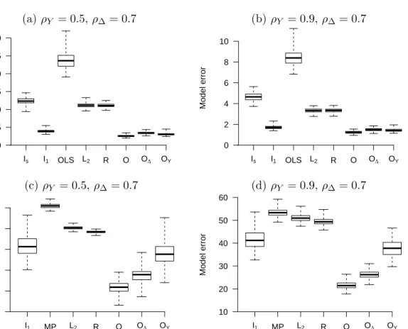
when the data generating model from Section 3.5.1 was used. In (a) and (b), n = 100, p = 60, q = 60, and s∗ = 0.1. In (c) and (d), n = 50,

p = 200, q = 200, and s∗ = 0.03. The estimator OLS is ordinary least squares, MP is Moore–Penrose least squares,L2isqunivariate response ridge

regressions with tuning parameters chosen separately, and R is multivariate ridge regression with one tuning parameter. . . 36 3.2 Boxplots of the observed model errors from 200 independent replications

when the data generating model from Section 3.5.2 was used. In (a) and (b),

n = 100, p = 60, q = 60, and s∗ = 0.1. In (c) and (d), n = 50, p = 200,

q = 200, ands∗ = 0.03. The estimators are defined in Section 3.5.1 and the caption of Figure 3.1. . . 38 3.3 Boxplots of the observed model errors from 200 replications whenn= 100, p=

20, q = 20, r∗ = 4. In (a) and (b), the data generating model from tion 3.5.3 was used. In (c) and (d), the data generating model from Sec-tion 3.5.4 was used. The estimator RR is likelihood-based reduced-rank for-ward regression (Izenman, 1975; Reinsel and Velu, 1998) and OLS is ordinary least squares. . . 40

(13)

List of Figures xi

3.4 A heatmap displaying the number of replications out of 1000 for which entries in the inverse regression’s coefficient matrix were estimated to be nonzero by

I2 for Chromosome 17. Black denotes 1000 and white denotes zero. The

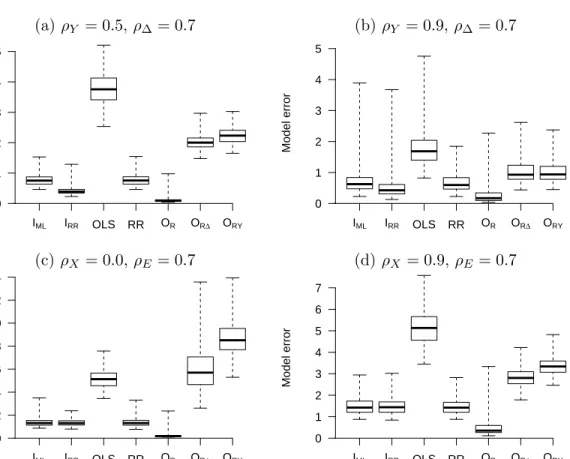
genes were sorted by hierarchical clustering. . . 44 4.1 Misclassification rates and Frobenius norm error averaged over 100

replica-tions with p = 200 for Models 1 and 2. The methods displayed are the estimator we proposed in Section 4.2.2 (dashed and ), the L1-penalized

Gaussian likelihood estimator (dashed and N), the Ledoit-Wolf-type estima-tor from (4.12) (dashed and ), Bayes (solid and

∗

), the method proposed by Guo (2010) (dots and_#), the method proposed by Mai et al. (2015) (dots and 4), and the method proposed by Witten and Tibshirani (2011) (dots and ). . . 57 4.2 True positive and true negative rates averaged over 100 replications with

p = 200 for Model 1 in (a) and (c); and for Model 2 in (b) and (d). The methods displayed are the estimator we proposed in Section 4.2.2 (dashed and ), the method proposed by Guo (2010) (dots and_#), and the method proposed by Mai et al. (2015) (dots and4). . . 58 4.3 Model sizes and misclassification rates from 100 random training/testing

splits with k = 100 (dark grey), k = 200 (grey), and k = 300 (light grey). Guo is the method proposed by Guo (2010), Mai is the method proposed by Mai et al. (2015), Glasso is the L1-penalized Gaussian likelihood precision matrix estimator, Ours is the estimator we propose Section 4.2.2, and Witten is the method proposed by Witten and Tibshirani (2011). . . 61 B.1 Boxplots of the observed model errors from 200 replicationswhen the data

generating model from Appendix B.1 is used. In (a) and (b),n= 100, p= 60, q = 60, s∗ = 0.1, and ν = 3. In (c) and (d), n = 50, p = 200, q = 200,

(14)

List of Figures xii

B.2 Boxplots of the observed model errors from 200 replications where (a), (b)

n= 100, p= 60, q= 60, s∗ = 0.1,ν = 10; (c), (d) n= 50, p= 200, q= 200,

s∗= 0.03, ν = 10; and the data generating model from Appendix B.1 is used. 84 B.3 Boxplots of the observed model errors from 200 replications wherethe data

generating model from Section 3.5.1 was used. In (a)–(c), n= 100, p= 60, q = 60, ands∗= 0.1. In (d)–(f), n= 50, p= 200, q= 200, and s∗ = 0.03. . . 86 B.4 Boxplots of the observed model errors from 200 replicationswhen the data

generating model from Section 3.5.2 is used. In (a)–(c), n = 100, p = 60, q = 60, ands∗= 0.1. In (d)–(f), n= 50, p= 200, q= 200, and s∗ = 0.03. . . 87 B.5 Boxplots of the observed model errors from 200 replications whenn= 100, p=

20, q= 20. In (a)–(d), the data generating model from Section 3.5.3 was used. In (e) and (f), the data generating model from Section 3.5.4 was used. . . . 88

(15)

Chapter 1

Overview

In recent decades, high-dimensional data analysis has emerged as an important area of research in statistics. Enabled by advances in computing and storage, researchers are able to collect more data about each subject than ever before. To make use of this data, statisticians need to develop new statistical methods and algorithms that address the computational and inferential challenges posed by high-dimensionality. They must must also consider whether certain modeling assumptions, such as sparsity, are appropriate or useful for a given application.

In this dissertation, we propose computationally efficient, model-based methods for clas-sification, multivariate response linear regression, and precision (inverse covariance) matrix estimation. The latter two methods acknowledge that in certain applications, the popular assumption of sparsity may not be appropriate or useful and proposes new methods for these cases. Because these methods address different problems, we provide background and a brief review of the relevant literature in each of the subsequent chapters separately.

In Chapter 2, we propose a model-based method for classification when the predictor is matrix-valued, e.g. an image of a handwritten digit. We fit the linear discriminant analysis model by maximizing a penalized matrix-normal log-likelihood. Specifically, we use penalties that encourage zeros in the precision matrix estimator and entrywise equality in pairs of response category mean matrix estimators. For one subproblem of our blockwise-coordinate descent algorithm, we use an alternating minimization algorithm, proposed by Tseng (1991), that scales more efficiently than the majorize-minimize algorithm used to solve

(16)

Chapter 1. Overview 2

special cases of our subproblem. Our proposed method can be generalized to the quadratic discriminant analysis model and can be adapted for classification when the predictor is a multidimensional array, such as in fMRI or video data. This chapter is based on the work in Molstad and Rothman (2016b).

In Chapter 3, which appears in Molstad and Rothman (2016a), we propose a new method for fitting the multivariate response linear regression model in high-dimensional settings without relying on the popular assumption that the regression coefficient matrix is sparse or has small Frobenius norm. Instead, we assume that predictors and responses have a joint multivariate normal distribution and propose to indirectly estimate the regression coefficient matrix by estimating the conditional distribution of the predictors given the response, i.e, theinverse regression. This allows us to fit a parsimonious inverse regression model when the forward regression is not parsimonious. We justify our approach by deriving a convergence rate bound for our indirect estimator. Through extensive simulation studies, we show that our indirect estimator can outperform popular direct estimators in finite samples. Our real data application suggests that our method is especially useful for virtual comparative genomic hybridization (Geng et al., 2011), a method for predicting genetic abnormalities from gene expression data.

In Chapter 4, we propose a new precision matrix estimator for applications when only a characteristic of the precision matrix is needed for prediction. The characteristics we consider are linear or affine functions evaluated at the precision matrix. We propose to estimate the population precision matrix by minimizing the normal negative log-likelihood plus anL1penalty on the characteristic evaluated at the optimization variable corresponding

to the precision matrix. To compute our estimator, we use an alternating direction method of multipliers algorithm that replaces one primal variable update with an approximation based on the majorize-minimize principle. This allows each step of algorithm to be solved in closed form. We also study the statistical properties of our estimator in terms of the sparsity of the characteristic. Specifically, we establish convergence rate bounds for our precision matrix estimator and the characteristic. Unlike existing methods for directly estimating linear or affine functions of the precision matrix, our estimator is applicable to a wide class

(17)

Chapter 1. Overview 3

of problems in multivariate analysis. In simulation studies, we show that for some linear discriminant analysis data generating models, our method has better classification accuracy than relevant competitors.

(18)

Chapter 2

A penalized likelihood method for

classification with matrix-valued

predictors

2.1 Introduction

We propose a method for classification when the predictor is matrix valued, e.g. classifica-tion of hand-written letters. Standard vector-valued predictor classificaclassifica-tion methods, such as logistic regression and linear discriminant analysis, could be applied, but they would not take advantage of the matrix structure.

Logistic regression based methods for classification with a matrix-valued predictor have been proposed. Zhou and Li (2014) proposed a nuclear norm penalized likelihood estimator of the regression coefficient matrixB∗ ∈Rr×cin a generalized linear model, where the value of the matrix predictorx ∈_Rr×c _{enters the model through the trace of}_BT

∗x. In the same setup, Hung and Wang (2013) assumed that vec(B∗) =β∗⊗α∗where vec stacks the columns of its argument, α∗ ∈Rr, β∗ ∈ Rc, and ⊗ is the Kronecker product. This decomposition was also studied in the dimension reduction literature (Li et al., 2010).

There also exist non-likelihood based methods for classification with a matrix-valued predictor. These approaches modify Fisher’s linear discriminant criterion, e.g. 2D-LDA (Li and Yuan, 2005), matrix discriminant analysis (Zhong and Suslick, 2015), and penalized matrix discriminant analysis (Zhong and Suslick, 2015).

(19)

2.1. Introduction 5

We propose a penalized likelihood method for classification with a matrix-valued pre-dictor. Our method estimates the parameters in the linear discriminant analysis model. Let xi ∈ Rr×c be the measured predictor for the ith subject and let yi ∈ {1, . . . , J} be the measured categorical response for the ith subject (i = 1, . . . , n). We assume that (x1, y1), . . . ,(xn, yn) are a realization of n independent copies of (X, Y) with the following distribution. The marginal distribution of Y is defined by P(Y = j) = πj (j = 1, . . . , J), where theπj’s are unknown; and

vec(X)|Y =j∼Nrc{vec (µ∗j),Σ∗}, j= 1, . . . , J, (2.1) whereµ∗j ∈Rr×cis the unknown mean matrix for thejth response category, and Σ∗ is the unknownrcby rccovariance matrix.

We make the simplifying assumption that

Σ−∗1= ∆∗⊗Φ∗, (2.2)

which is equivalent to Σ∗ = ∆−∗1⊗Φ∗−1, where Φ∗ is an unknownr by r precision matrix with P

a,b|Φ∗a,b|=r, and ∆∗ is an unknown c by c precision matrix. The norm condition on Φ∗ is added for identifiability: see Ro´s et al. (2016) for more on identifiability under (2.2). This simplification of a covariance matrix makes the conditional distributions in (2.1) become matrix normal (Gupta and Nagar, 2000). This exploits the matrix structure of the predictor by reducing the number of parameters in the precision matrix fromO(r2c2) toO(r2+c2).

Several authors have proposed and studied penalized likelihood estimators of Φ∗and ∆∗ when J = 1 (Allen and Tibshirani, 2010; Zhang and Schneider, 2010; Tsiligkaridis et al., 2012; Leng and Tang, 2012; Zhou, 2014).

In this chapter, we propose a penalized likelihood method to fit (2.1) with the as-sumption in (2.2). Our penalties encourage fitted models that can be easily interpreted by practitioners. We use a blockwise coordinate descent algorithm to compute our esti-mators. To exploit (2.2) computationally, we use an alternating minimization algorithm

(20)

2.2. Penalized likelihood estimation 6

(Tseng, 1991) in one of our block updates. This algorithm scales more efficiently than other popular algorithms, which makes our method computationally feasible for high-dimensional problems. We show that our algorithm has the same computational complexity order as the unpenalized likelihood version, which also requires a blockwise coordinate descent algorithm (Dutilleul, 1999).

2.2 Penalized likelihood estimation

2.2.1 Proposed method

Let Sm+ be the set of symmetric and positive definite m by m matrices. The maximum

likelihood estimators of theµ∗j’s, Φ∗, and ∆∗ minimize the functiong: (Rr×c)J×Sr+×Sc+ → Rdefined by g(µ,Φ,∆) = 1 n J X j=1 " _n X i=1 1(yi=j)tr Φ(xi−µj)∆(xi−µj)T #

−clog det(Φ)−rlog det(∆),

whereµ= (µ1, . . . , µJ). We propose the penalized likelihood estimators defined by

ˆ µ,∆ˆ,Φˆ= arg min (µ,Φ,∆)∈T    g(µ,Φ,∆) +λ1 X j<m kwj,m◦(µj−µm)k1+λ2k∆⊗Φk1    , (2.3) subject to kΦk1 =r

whereT = (Rr×c)J×Sr+×Sc+;◦is the Hadamard product; k · k1 is the sum of the absolute

values of the entries of its argument;λ1and λ2 are nonnegative tuning parameters; and the wj,m’s are r by c user-specified weight matrices.

The first penalty in (2.3) encourages solutions for which pairs of the mean matrix esti-mates have some equal entries, where this equality occurs in the same locations. Without the first penalty, i.e. λ1 = 0, the proposed estimators of theµ∗j’s are sample mean matrices. If λ1 > 0, then the proposed estimators of the µ∗j’s are affected by the estimators of Φ∗ and ∆∗.

(21)

2.2. Penalized likelihood estimation 7

We recommend selecting weights similar to those prescribed by Guo (2010). We suggest using w_j,m−1 = |x¯j −x¯m|,1 ≤ j < m ≤ J where ¯xj = Pn_i₌₁1(yi = j)xi. Alternatively, one could use weights based on t-test statistics or could use weights that incorporate prior information.

The second penalty in (2.3) has a simple impact: for sufficiently large values ofλ2, some

of the entries in the estimate of ∆∗ ⊗Φ∗ are zero, which occurs if and only if either the estimate of ∆∗or the estimate of Φ∗has some zero entries. To encourage zeros in estimates of Φ∗or ∆∗ separately, one could use two separateL1 penalties. Our computational algorithm can be easily adapted to accommodate this case.

The tuning parametersλ1 andλ2 can be chosen by minimizing the misclassification rate on a validation set.

2.2.2 Related work

Xu et al. (2015) proposed fitting the standard linear discriminant analysis model for a vector-valued predictor by penalized likelihood. We can express their parameter estimates in our matrix-predictor setup by setting the number of columns of the matrix predictor to one. Specifically, withc= 1 and ∆ = 1, Xu et al. (2015) parameter estimates are

arg min (µ,Φ)∈(Rr)J×Sr+    g(µ,Φ,1) +λ1 X j<m kwj,m◦(µj−µm)k1+λ2 X a6=b |Φab|    . (2.4)

One could view our method as the matrix-valued predictor extension of the method of Xu et al. (2015). Guo (2010) proposed a method that solves a restricted version of (2.4), where Φ is fixed at a diagonal matrix with pooled sample precision estimates on its diagonal.

Computationally, the algorithms proposed by Xu et al. (2015) and Guo (2010) for solving (2.4) suffer from numerical instability and do not scale efficiently for application to (2.3). In our simulation studies, we compare our proposed method to several competitors, including the method of Guo (2010). The method of Xu et al. (2015) is too slow computationally for the dimensions we consider, so we only use it in a special case when Σ∗ is known.

(22)

2.3. Computation 8

2.3 Computation

2.3.1 Overview

To solve (2.3), we use a block-wise coordinate descent algorithm. Each block update is a convex optimization problem. In the subsequent subsections, we show that updates for Φ and ∆ can be expressed as the well-studied L1-penalized Gaussian likelihood precision matrix estimation problem. We also use an alternating minimization algorithm for the block update for µ. The algorithm to compute our estimator, along with a set of auxiliary functions, is implemented in the Rpackage MatrixLDA, which is available on CRAN.

2.3.2 Updates for Φ and ∆

We first derive the update for Φ. Define GL(S, τ) as

GL(S, τ) = arg min

Θ∈_S+

{tr(SΘ)−log det(Θ) +τkΘk1}, (2.5)

whereS is some given nonnegative definite matrix andτ is a nonnegative tuning parameter. The optimization problem in (2.5) is theL1-penalized Gaussian likelihood precision matrix

estimation problem. Many algorithms and efficient software exist to solve (2.5): one good example is the graphical-lasso of Friedman et al. (2008).

Let f be the objective function in (2.3). Suppose ∆ andµ are fixed. The minimizer of

f with respect to Φ is ˜ Φ = arg min Φ∈_Sr +    1 n J X j=1 " _n X i=1 1(yi=j)tr Φ(xi−µj)∆(xi−µj)T # −clog det(Φ) +λ2kΦ⊗∆k1    . (2.6)

Using the fact that kΦ⊗∆k1=kΦk1k∆k1 and

1 n J X j=1 " _n X i=1 1(yi=j)tr Φ(xi−µj)∆(xi−µj)T # =c tr{ΦSφ(µ,∆)},

(23)

2.3. Computation 9 where Sφ(µ,∆) = 1 nc J X j=1 ( _n X i=1 1(yi=j) (xi−µj) ∆ (xi−µj)T ) , we can express (2.6) as arg min Φ∈_Sr + tr{ΦSφ(µ,∆)} −log det(Φ) + λ1k∆k1 c kΦk1 = GL Sφ(µ,∆), λ1k∆k1 c .

After computing ˜Φ with ∆ fixed, we can enforce the constraint kΦk1 = r using a simple

normalization: we replace ( ˜Φ,∆) with ( ¯Φ,∆), where¯

¯ Φ = r kΦ˜k1 ˜ Φ, ∆ =¯ kΦ˜k1 r ∆.

This ensures that kΦ¯k = r without changing the objective function because f(µ,∆,Φ) =˜

f(µ,∆¯,Φ).¯

Using a similar argument, the minimizer of f with respect to ∆ with µand Φ fixed is

˜ ∆ = GL Sδ(µ,Φ), λ1kΦk1 r , where Sδ(µ,Φ) = 1 nr J X j=1 ( _n X i=1 1(yi =j) (xi−µj)TΦ (xi−µj) ) . 2.3.3 Update for µ

Let ∆ and Φ be fixed. The minimizer off with respect toµis

arg min µ∈R(r×c)J 1 n J X j=1 ( _n X i=1 1(yi =j)tr Φ(xi−µj)∆(xi−µj)T ) +λ1 X j<m kwj,m◦(µj−µm)k1. (2.7)

Special cases of (2.7) have been solved using the majorize-minimize principle (Lange, 2016), where the penalty is majorized by its local-quadratic approximation at the current iterate

(24)

2.3. Computation 10

(Hunter and Li, 2005). For example, Xu et al. (2015) solved (2.7) when c= 1 and ∆ = 1; and Guo (2010) solved (2.7) when c = 1, ∆ = 1, and Φ was diagonal. However, this majorize-minimize algorithm suffers from numerical instability when iterates forµj andµm are similar from some (j, m). Moreover, if we were to apply the majorize-minimize algorithm to solve (2.7), then each iteration would would have worst case computational complexity

O(r2c2).

Instead of using an majorize-minimize algorithm, we use an alternating minimization algorithm (Tseng, 1991; Chi and Lange, 2015) to solve (2.7). Our algorithm for solving (2.7) is more numerical stable, each iteration has worst case computational complexity

O(r2c+c2r), and has a quadratic rate of convergence when implemented with the acceler-ations proposed by Goldstein et al. (2014). Both the majorize-minimize algorithm and our alternating minimization algorithm require one inversion of ∆ and of Φ.

Similarly to the setup of the alternating direction method of multipliers algorithm (Boyd et al., 2011), we first express (2.7) as a constrained optimization problem:

minimize (µ,Θ)∈G g(µ,Φ,∆) +λ1 X j<m kwj,m◦Θj,mk1 (2.8) subject to Θj,m=µj −µm 1≤j < m≤J,

whereG=R(r×c)J×R(r×c)J(J−1)/2 and Θ = (Θ1,2, . . . ,ΘJ−1,J).The augmented Lagrangian for (2.8), using notation similar to Chi and Lange (2015), is

F_ρ(µ,Θ,Γ) =g(µ,Φ,∆) +λ1 X j<m kwj,m◦Θj,mk1 +X j<m tr ΓT_j,m(Θj,m−µj+µm) + ρ 2 X j<m kΘj,m−µj +µmk2F,

for step size parameter ρ > 0 and Lagrangian variables Γj,m ∈ Rr×c for 1 ≤j < m ≤ J. Letting the superscript t denote the value of the t-th iterate of an optimization variable,

(25)

2.3. Computation 11

the alternating minimization algorithm updating equations are

µ(t+1) = arg min µ∈R(r×c)J F₀µ,Θ(t),Γ(t), (2.9) Θ(t+1) = arg min Θ∈_R(r×c)J(J−1)/2 Fρ µ(t+1),Θ,Γ(t) , (2.10) Γ(_j,mt+1) = Γ(_j,mt) +ρ Θ_j,m(t+1)−µ_j(t+1)+µ(_mt+1) for 1≤j < m≤J,

until convergence. The alternating direction method of multipliers algorithm modifies (2.9) by usingF_ρrather thanF₀. The advantage of using F₀ is that we avoid solving anrc×rc

linear system of equations at complexityO(r2c2) when using the Kronecker structure. Using

F₀ also allows the updates for µ1, . . . , µJ to be computed in parallel with closed form solutions for each. Two conditions for the convergence of alternating minimization are that

g is strongly convex (Tseng, 1991), which it is in our case, and that ρ is sufficiently close to zero. We provide a computable bound on the step size ρ to ensure convergence of our alternating minimization algorithm in the subsequent section.

The computational advantage of alternating minimization over alternating direction method of multipliers was also recognized by Chi and Lange (2015) in the context of convex clustering. They found that the simplification of (2.9) relative to the alternating direction method of multipliers version yielded a substantially more efficient algorithm.

Using the first order optimality condition for (2.9),

µ(_jt+1) = ¯xj + 1 2ˆπj Φ−1   X {m:m>j} Γ(_j,mt) − X {m:m<j} Γ(_m,jt)  ∆ −1 _j_{= 1}_{, . . . , J,} _(2.11) where ˆπj =nj/n forj= 1, . . . , J.

The zero subgradient equation for (2.10) is

ρΘ(_j,mt+1)+ Γ(_j,mt) −ρ µ(_jt+1)−µ(_mt+1) + n λ1wj,m◦h Θ(_j,mt+1) o = 0, (2.12)

(26)

2.3. Computation 12

whereh:Rr×c→Rr×cand for all (s, t)∈ {1, . . . r} × {1, . . . , c}, [h(x)]_s,t=    sign(xs,t) :xs,t6= 0 [−1,1] :xs,t= 0 .

Tibshirani (1996), among others, have shown that (2.12) can be solved using the soft-thresholding operator: soft(x, τ) = max(|x| −τ,0)sign(x). The update for Θj,m is

Θ(_j,mt+1)= soft µ(_jt+1)−µ(_mt+1)−ρ−1Γ(_j,mt) ,λ1 ρ wj,m ,

where soft is applied elementwise.

We use an accelerated variation of the algorithm presented in this section to solve (2.7). This is based on Goldstein et al. (2014) with simple restarting rules described by O’Donoghue and Candes (2015). Further details about our implementation are given in the subsequent section.

2.3.4 Summary

The block-wise coordinate descent algorithm for solving (2.3) is summarized in Algorithm 1.

Algorithm 1 Blockwise coordinate descent algorithm for (2.3) Initialize ∆(0) ∈_S+

c, Φ(0) ∈S+r such that kΦ(0)k1 =r. Set m= 0.Repeat Step 1 - 5 until

convergence.

Step 1. Compute µ(m+1)= arg min_µ_∈_R(r×c)J g µ,Φ(m),∆(m)

+λ1

P

j<mkwj,m◦(µj−µm)k1 using

the algorithm in Section 2.3.3;

Step 2. Compute ˜∆ = GLSδ µ(m+1),Φ(m) , λ2 ; Step 3. Compute ˜Φ = GL n Sφ µ(m+1),∆˜ ,λ2 ck∆˜k1 o ; Step 4. Set ∆(m+1)= kΦ˜_rk1∆, Φ˜ (m+1) = r kΦ˜k1Φ;˜ Step 5. Replacem withm+ 1.

To get initial values Φ(0)and ∆(0), we run the maximum likelihood algorithm (Dutilleul, 1999) until a mild convergence tolerance is reached, and use Φ(0) = diag(ΦMLE) and ∆(0)= diag(∆MLE) where ΦMLE,∆MLE are the final iterates.

(27)

2.3. Computation 13

Let k(_φm) = ϕmin(Φ(m)) and k_δ(m) = ϕmin(∆(m)), where ϕmin(·) denotes the minimum

eigenvalue of its argument. For the (m + 1)th update of µ, if we select the step size parameter ρ(m+1)∈ 0, min j {πˆj}4k (m) φ k (m) δ /J , (2.13)

then the alternating minimization algorithm converges (Tseng, 1991; Chi and Lange, 2015). One can verify that (2.7) and (2.13) satisfy the conditions for convergence stated in Section 6.2 of the Supplemental Material of Chi and Lange (2015) using an argument similar to theirs. The minimum eigenvalues of Φ(m) and ∆(m) are positive as long as initializers Φ(0) and ∆(0) are positive definite. When k(_δm) andk(_φm) are positive, g is strongly convex in µ, which is required for convergence.

In practice, we find it better to use ρ an order of magnitude smaller than the upper bound in (2.13), i.e., we use ρ(m+1) = (minj{ˆπj}4k

(m)

φ k

(m)

δ )/(10J) to ensure numerical stability. Although the step size ρ(m+1) _{may be small when Φ}(m) _{and ∆}(m) _{are dense, we}

find that when using accelerations and warm-starts, the small step size is not problematic. We use an accelerated version of the alternating minimization algorithm proposed by Goldstein et al. (2014), which was also used by Chi and Lange (2015). O’Donoghue and Candes (2015) showed that acceleration restarts imposed after a fixed number of iterations can decrease the number of iterations required for convergence. In our implementation of the alternating minimization algorithm, we restart the accelerations after 200 iterations. We warm-start the (m+ 1)th update ofµ by initializing the Lagrangian variables at their final iterates from the mth update.

At convergence of the alternating minimization algorithm, zeros in the final iterate of Θj,m do not correspond to exact entrywise equality in the final iterates forµj and µm. To enforce equality at the solution, we use simple thresholding.

(28)

2.4. Simulations 14

2.3.5 Computational complexity

Solving (2.3) with λ1 =λ2 = 0, i.e. maximum likelihood estimation, also requires a

block-wise coordinate descent algorithm (Dutilleul, 1999). The maximum-likelihood blockblock-wise co-ordinate descent algorithm has computational complexity of orderO(nr2c+nc2r+r3+c3). The first two terms come from computing the sample covariance matrices Sφ and Sδ, and the last two terms come from inverting Sφ andSδ.

Our algorithm’s computational complexity is alsoO(nr2c+nc2r+r3+c3). We compute

Sφ and Sδ and the graphical-lasso algorithm that we use is known to have worst case complexityO(p3) for a estimating ap×pprecision matrix (Witten et al., 2011). In addition, for each µ update, we compute eigendecompositions of the iterates for Φ and ∆. The alternating minimization algorithm costs O(r2c+c2r) when implemented in parallel.

The magnitude of tuning parameters effects the computing time of our algorithm. Gen-erally, smaller values ofλ2 take longer.

2.4 Simulations

2.4.1 Models

For 100 independent replications, we generated a realization ofn=ntrain+nvalidate+ntest

independent copies of (X, Y), where we set ntrain =nvalidate = 75, and ntest = 1000. The

categorical responseY has support{1,2,3}with probabilitiesπ∗1=π∗2 =π∗3 = 1/3.Then

vec (X)|Y =j∼Nrc{vec (µ∗j),Σ∗},

whereµ∗1, µ∗2,and µ∗3 are only different in one 4×4 submatrix, whose position is chosen

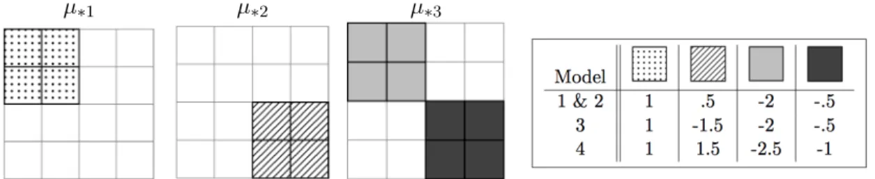
randomly in each replication. We used multiple choices for the entries in this submatrix, which are displayed in Figure 2.1. All other mean matrix entries were set to zero. We consider four covariance models:

Model 1. Σ∗ = ∆∗⊗Φ∗ where Φ∗ has (a, b)th entry 0.7|a−b|and ∆∗ has (c, d)th entry 0.7×1(c6=d) + 1(c=d).

(29)

2.4. Simulations 15

Model 2. Σ∗ = ∆∗⊗Φ∗ where Φ∗ has (a, b)th entry 0.7|a−b| and ∆∗ is block-diagonal where ∆∗ can be expressed elementwise:

∆c,d=          1 ifc=d

0.7 ifµ∗j,a,c 6=µ∗m,a,d for any a∈ {1, . . . , r} and 1≤j < m≤J 0 otherwise

.

Model 3. Σ∗ corresponds to the covariance model

Cov(Xa,b, Xc,d|Y =j) ={0.5I(b6=d) +I(b=d)}

(ρbρd)|a−c| 1−ρbρd

,

where ρ1, . . . , ρc are c equally spaced values between 0.5 and 0.9. The matrix Σ∗ is positive definite when r = c with c = {8,16,32,64}, and when r = 32 with c =

{8,16,32,64}.

Model 4. Σ∗ corresponds to the covariance model

Cov(Xa,b, Xc,d|Y =j) =          1 if (a, b) = (c, d)

0.5 ifµ∗j,a,b=6 µ∗m,c,d for any 1≤j < m≤J 0 otherwise

.

In Model 3, if ρk = ρ for all k ∈ {1, . . . , c}, then Σ∗ has the decomposition (2.2) corresponding to Φ∗with an AR(1) structure and ∆∗ with a compound symmetric structure (Mitchell et al., 2006). However, whenρk 6=ρ, Σ∗ does not have decomposition (2.2): the correlation between any two entries in the same row depends on the column and vice versa. Model 4 is therc−variate normal model similar to the first model used in the simulations from Xu et al. (2015).

2.4.2 Methods

We consider the following model-based methods for fitting the linear discriminant analysis model:

(30)

2.4. Simulations 16

µ∗1 µ∗2 µ∗3

Figure 2.1: The 4×4 submatrix whereµ∗1,µ∗2, andµ∗3 differ. White corresponds to zero

and the legend gives the values corresponding to the highlighted cells for each model. • Bayes. The Bayes rule, i.e., Σ∗,µ∗, and π∗j known for j= 1, . . . , J;

• MN. The maximum likelihood estimator of (2.1) under (2.2), i.e., the matrix-normal maximum likelihood estimator;

• Guo. The sparse na¨ıve Bayes type-estimator proposed by Guo (2010) with tuning parameter chosen to minimize misclassification rate on the validation set;

• vec-SURE. The SURE independence screening method proposed by Pan et al. (2016) with model sizes chosen to minimize misclassification rate on the validation set; • MN-SURE. The matrix-normal extension of the SURE independence screening

estima-tor proposed by Pan et al. (2016) with model sizes chosen to minimize misclassification error on the validation set.

• PMN(µ). The estimator defined by (2.3) withµ=µ∗ fixed andλ2chosen to minimize

misclassification rate on the validation set;

• PMN(Σ) / Xu(Σ). The estimator defined by (2.3) with Φ = Φ∗ and ∆ = ∆∗ fixed when Σ∗ = ∆∗ ⊗Φ∗; the estimator defined by (2.4) with ˆΣ = Σ∗ fixed when Σ∗ 6= ∆∗⊗Φ∗; andλ1 chosen to minimize misclassification rate on the validation set;

• PMN. The estimator defined by (2.3) with tuning parameters chosen by minimizing misclassification rate on the validation set.

The methods PMN(µ) and PMN(Σ) / Xu(Σ) both use some oracle information and were included to study how estimatingµ∗, ∆∗, and Φ∗ simultaneously affect classification

(31)

accu-2.4. Simulations 17

racy. We refer to these method as part-oracle matrix-LDA methods. We refer to Guo and vec-SURE as vector-LDA methods; MN and MN-SURE as non-oracle matrix-LDA meth-ods. MN-SURE is a matrix-normal generalization of the screening method proposed by Pan et al. (2016).

Following Guo (2010), we use a validation set to select tuning parameters. The candidate set for tuning parameters was {2x:x=−12,−11.5, . . . ,11.5,12}. Candidate model sizes for vec-SURE and MN-SURE were {0,1, . . . ,25}, where model size refers to the number of pairwise nonzero mean differences based on thresholding.

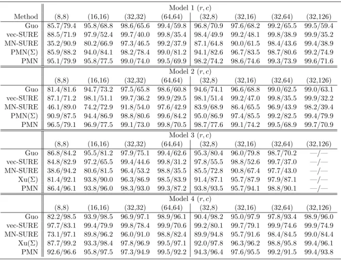
Table 2.1: True negative rates and true positive rates, respectively, averaged over the 100 replications for the models from Section 2.4.1.

Model 1 (r, c) Method (8,8) (16,16) (32,32) (64,64) (32,8) (32,16) (32,64) (32,126) Guo 85.7/79.4 95.8/68.8 98.6/65.6 99.4/59.8 96.8/70.9 97.6/68.2 99.2/65.5 99.5/59.4 vec-SURE 88.5/71.9 97.9/52.4 99.7/40.0 99.8/35.4 98.4/49.9 99.2/48.1 99.8/38.9 99.9/35.2 MN-SURE 35.2/90.9 80.2/66.9 97.3/46.5 99.2/37.9 87.1/64.8 90.0/61.5 98.4/43.6 99.4/38.9 PMN(Σ) 85.9/88.2 94.0/84.1 98.2/78.4 99.0/81.2 94.1/82.6 96.7/83.5 98.7/80.6 99.2/74.9 PMN 95.1/79.9 95.8/77.5 99.0/74.0 99.5/69.9 98.2/74.2 98.6/74.6 99.3/73.9 99.6/71.6 Model 2 (r, c) (8,8) (16,16) (32,32) (64,64) (32,8) (32,16) (32,64) (32,126) Guo 81.4/81.6 94.7/73.2 97.5/65.8 98.6/60.8 94.6/74.1 96.6/68.8 99.0/62.5 99.0/63.1 vec-SURE 87.1/71.2 98.1/51.1 99.7/36.2 99.9/29.5 98.1/51.4 99.2/47.0 99.8/35.5 99.9/32.2 MN-SURE 46.1/89.0 74.2/72.9 91.8/54.0 97.6/42.9 83.9/68.9 86.4/65.5 96.9/43.9 98.2/39.4 PMN(Σ) 90.9/87.5 94.4/86.9 98.8/80.6 99.6/84.2 95.0/86.9 97.4/85.5 99.2/82.5 99.4/79.9 PMN 96.5/79.1 96.9/77.5 99.1/73.0 99.8/70.5 98.7/77.6 99.1/74.2 99.5/68.9 99.7/70.9 Model 3 (r, c) (8,8) (16,16) (32,32) (64,64) (32,8) (32,16) (32,64) (32,126) Guo 86.8/84.2 95.5/81.2 97.9/75.1 99.4/62.6 95.3/80.4 96.0/79.8 98.7/70.2 —/— vec-SURE 84.8/82.9 97.2/65.5 99.4/44.6 99.8/31.2 97.8/55.5 98.8/52.6 99.7/37.0 —/— MN-SURE 38.6/94.2 80.6/81.5 96.4/53.2 98.8/35.5 85.5/72.8 90.8/67.4 97.7/43.0 —/— Xu(Σ) 81.4/92.1 93.8/90.0 96.3/86.9 98.5/83.9 91.4/87.1 95.7/87.9 97.9/87.1 —/— PMN 86.4/96.1 93.8/96.0 98.3/93.0 99.3/87.2 93.8/93.5 95.7/94.1 98.8/90.1 —/— Model 4 (r, c) (8,8) (16,16) (32,32) (64,64) (32,8) (32,16) (32,64) (32,126) Guo 82.2/98.5 93.9/98.5 96.9/97.1 98.9/96.1 90.4/98.2 95.0/97.9 97.8/93.4 98.9/96.0 vec-SURE 97.7/83.1 99.4/79.9 99.8/78.4 99.9/70.6 99.2/80.1 99.7/79.1 99.9/74.6 99.9/74.9 MN-SURE 73.1/97.1 89.8/96.2 96.0/91.0 98.8/82.4 89.9/94.8 95.7/91.6 98.4/84.5 99.0/84.4 Xu(Σ) 87.7/99.2 93.3/98.4 97.8/96.9 99.5/97.1 92.0/97.8 96.3/96.2 98.8/95.8 99.4/96.1 PMN 92.6/96.6 95.8/97.5 97.3/94.9 99.5/92.2 94.3/96.4 97.6/95.5 99.2/91.5 99.4/93.8

(32)

2.4. Simulations 18

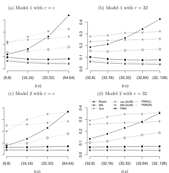
(a) Model 1 withr=c (b) Model 1 withr = 32

(r,c) A v er age misclassification r ate (8,8) (16,16) (32,32) (64,64) 0.0 0.1 0.2 0.3 0.4 ● ● ● ● (r,c) (32,8) (32,16) (32,32) (32,64) (32, 126) 0.0 0.1 0.2 0.3 0.4

(c) Model 2 with r=c (d) Model 2 with r= 32

(r,c) A v er age misclassification r ate (8,8) (16,16) (32,32) (64,64) 0.0 0.1 0.2 0.3 0.4 ● ● ● ● (r,c) (32,8) (32,16) (32,32) (32,64) (32, 126) 0.0 0.1 0.2 0.3 0.4 Bayes MN Guo vec-SURE MN-SURE PMN PMN(Σ) PMN(M)

Figure 2.2: Misclassification rates averaged over 100 replications; (a) and (b) are for Model 1 and (c) and (d) for Model 2.

(33)

2.4. Simulations 19

2.4.3 Performance measures

To compare classification accuracy, we record the misclassification rate on the test set for each replication. We also measure identification of mean differences that are zero through both true positive and true negative rate. LetD(µ∗) =vec(µ∗1−µ∗2), . . . ,vec(µ∗(J−1)−µ∗J)

, and D(ˆµ) = vec(ˆµ1−µ2ˆ ), . . . ,vec(ˆµ(J−1)−µˆJ)

. We define the true positive rate of an estimator ˆµas card n (z, w) : [D(ˆµ)]_z,w 6= 0∩[D(µ∗)]_z,w 6= 0 o card n (z, w) : [D(µ∗)]_z,w 6= 0 o ,

where card denotes cardinality of a set. We similarly define the true negative rate of an estimator ˆµas card n (z, w) : [D(ˆµ)]_z,w = 0∩[D(µ∗)]_z,w = 0 o card n (z, w) : [D(µ∗)]_z,w = 0 o .

True positive and true negative rates together address mean difference estimation which we use as a measure of variable selection for comparison to the estimator of Guo (2010) and Pan et al. (2016).

2.4.4 Results

We display average misclassification rates for Models 1 and 2 in Figure 2.2. For Model 1, the matrix-normal maximum likelihood estimator tended to outperform the vector-LDA methods when r and c were small, but its average classification rate got worse as the dimensionality increases. The estimator proposed by Guo (2010) performs poorly when r

andcare small, but got worse more slowly than the other vector and non-oracle matrix-LDA methods. The misclassification rate of the Bayes rules suggests that as the dimensionality increases in Model 1, the optimal misclassification rate can be improved. Our method PMN had improved classification accuracy as bothr and c increased and performed similarly to PMN(Σ), which uses some oracle information.

True positive and true negative rate results are displayed in Table 2.1. For Model 1, PMN tended to have the second highest true negative rate behind vec-SURE, but tends

(34)

2.4. Simulations 20

to have higher true positive rate than all competing methods except PMN(Σ), which uses some oracle information.

Results were similar for Model 2. The matrix-normal variation of the SURE screening estimator of Pan et al. (2016) tended to perform best among the vector and non-oracle matrix-LDA methods. The estimator of Guo (2010) got worse the slowest amongst the vector-LDA methods. PMN performed as well as PMN(Σ), both of which performed more closely to PMN(µ) and the Bayes rule than for Model 1.

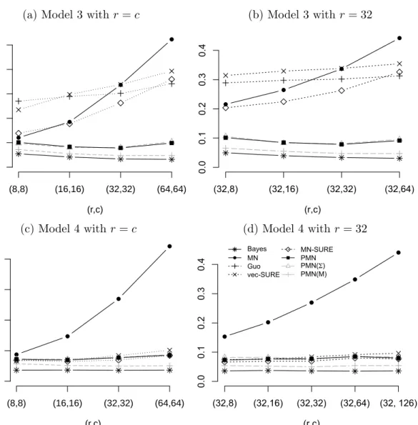
The misclassification rates for Models 3 and 4 are displayed in Figure 2.3. In Model 3, although Σ∗ does not have the Kronecker decomposition in (2.2), PMN outperformed all non part-oracle estimators. In terms of true positive and true negative rate results presented in Table 2.1, PMN performed similarly to Xu(Σ), both of which had higher true positive rate than competitors and true negative rate similar to vec-SURE. This suggests that even when (2.2) does not hold, our method can perform well in classification.

In Model 4, PMN performed similarly to the vector-LDA methods. MN-SURE was the best non-oracle method, which suggests that (2.2) may be a reasonable alternative to na¨ıve Bayes under high dimensionality. Like in Model 3, PMN performed similarly to Xu(Σ) in terms of true positive and true negative rates.

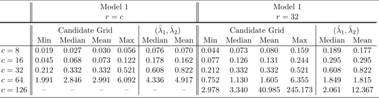
We also report timing results for all the settings in Model 1. In our simulations, we used a 12×12 grid of candidate tuning parameters (λ1, λ2) for our method. For each point on the grid, we compute the average computing time over the 100 replications. In Table 2.2 we report the minimum, maximum, mean, and median average computing times for all of the points on the grid computing using warm-starts. We also include median and mean average computing times (without warm-starts) for the tuning parameter pair selected by minimizing the misclassification rate on the validation set. In Figure 2.4, we show smoothed contour plots of average computing times for the cases wherer = 32 andc= 32 andc= 64.

All computations were performed on an Intel Core i7-3770 CPU at 3.4GHz with 8GB of RAM. Our package MatrixLDA was designed for computation on a single CPU, but the source code can be easily modified to allow for parallelization, which could reduce computing times.

(35)

2.4. Simulations 21

(a) Model 3 with r=c (b) Model 3 withr= 32

(r,c) A v er age misclassification r ate (8,8) (16,16) (32,32) (64,64) 0.0 0.1 0.2 0.3 0.4 0.5 ● ● ● ● (r,c) (32,8) (32,16) (32,32) (32,64) 0.0 0.1 0.2 0.3 0.4

(c) Model 4 with r=c (d) Model 4 with r= 32

(r,c) A v er age misclassification r ate (8,8) (16,16) (32,32) (64,64) 0.0 0.1 0.2 0.3 0.4 ● ● ● ● (r,c) (32,8) (32,16) (32,32) (32,64) (32, 126) 0.0 0.1 0.2 0.3 0.4 Bayes MN Guo vec-SURE MN-SURE PMN PMN(Σ) PMN(M)

Figure 2.3: Misclassification rates averaged over 100 replications; (a) and (b) are for Model 3 and (c) and (d) for Model 4.

(36)

2.4. Simulations 22

(a) Model 1 with (r, c) = (32,32) (b) Model 1 with (r, c) = (64,64)

0.20 0.25 0.30 0.35 0.40 0.45 0.50 0.55 −4 −3 −2 −1 0 1 −8 −7 −6 −5 −4 −3 log2(λ1) lo g2 ( λ2 ) 2 3 4 5 6 −4 −3 −2 −1 0 1 −8 −7 −6 −5 −4 −3 log2(λ1) lo g2 ( λ2 )

Figure 2.4: Smoothed contour plots of average computing times (in seconds) over 100 replications for each of 12×12 candidate grid points under Model 1 using warm-starts.

Table 2.2: Summary statistics for average computing time (in seconds) over 100 replications for PMN under Model 1. Candidate grid timings show the minimum, median, mean, and maximum average computing time over a 12×12 grid of candidate tuning parameters using warm-starts. The columns corresponding to (ˆλ1,λ2ˆ ) give the average computing time (without warm-start initialization) for the tuning parameter pair chosen to minimize the misclassification rate on the validation set.

Model 1 Model 1

r=c r= 32

Candidate Grid (ˆλ1,ˆλ2) Candidate Grid (ˆλ1,λ2)ˆ Min Median Mean Max Median Mean Min Median Mean Max Median Mean c= 8 0.019 0.027 0.030 0.056 0.076 0.070 0.044 0.073 0.080 0.159 0.189 0.177 c= 16 0.045 0.068 0.073 0.122 0.178 0.162 0.077 0.126 0.131 0.244 0.295 0.295 c= 32 0.212 0.332 0.332 0.521 0.608 0.822 0.212 0.332 0.332 0.521 0.608 0.822 c= 64 1.991 2.846 2.991 6.092 4.336 4.917 0.752 1.130 1.605 6.355 1.849 1.815 c= 126 – – – – – – 2.978 3.340 40.985 245.173 2.061 12.367

(37)

2.5. EEG data example 23

2.5 EEG data example

We analyzed the EEG data (https://kdd.ics.uci.edu/databases/eeg/eeg.html) also studied by Li et al. (2010) and Zhou and Li (2014). In the original study, 122 subjects, 77 of whom were alcoholics and 45 of whom were control, were exposed to stimuli while voltage was measured fromc = 64 channels on a subject’s scalp at r = 256 time points. Each subject underwent 120 trials. Each trial had one of three possible stimuli: single stimulus, two matched stimuli, or two unmatched stimuli. As in Li et al. (2010) and Zhou and Li (2014), we only analyze the single stimulus condition. Because each subject underwent multiple trials under the single stimulus condition, we use the within subject average over all single stimulus trials as the predictor and we use whether they were alcoholic or control as the response.

It is common to assume that (2.2) holds in the analysis of EEG data. For example, Zhou (2014) assumed that (2.2) holds when analyzing a single subject from this same dataset. It may also be reasonable to assume that only a subset of channels and time point combinations are important for discriminating between alcoholic and control response categories. Thus, the primary goal of our analysis is to identify a subset of channels and time point combinations that help explain how the alcoholics and controls react to the stimulus differently.

To demonstrate our method’s classification accuracy, we used the leave-one-out cross validation approach from Li et al. (2010) and Zhou and Li (2014). For k = 1, . . . ,122, we left out the kth observation and used the remaining 121 observations as training data. For eachk, we selected tuning parameters for use in (2.3) by minimizing 5-fold cross validation misclassification error on the training dataset. Our method correctly classified 97 of 122 observations. Li et al. (2010) and Zhou and Li (2014) reported correctly classifying 97 and 94 of 122, respectively. Li et al. (2010) used quadratic discriminant analysis after dimension-folding of the predictors, and Zhou and Li (2014) used logistic regression with spectral regularization of the coefficient matrix.

(38)

2.5. EEG data example 24 Channel Time (3.9 msec) 50 100 150 200 250 10 20 30 40 50 60 0 1 2 3 4 5 6 7 Channel 50 100 150 200 250 10 20 30 40 50 60 0.0 0.5 1.0 1.5 2.0 (a) (b)

Figure 2.5: (a) The absolute value of the sample mean differences between the alcoholic and control response categories. (b) The absolute value of the estimated mean differences from (2.3) based on the tuning parameter pair (λ1, λ2) = (0.15,5.66), which had leave-one-out

(39)

2.5. EEG data example 25

●

● _●

●

● ● ●

● ●

●

● _●

●

FP1 FP2 F7 F8 AF1 AF2 FZ F4 F3 FC6 FC5 FC1 FC2 T8 T7 C3 CZ C4 CP5 CP1 CP2 CP6 P3 PZ P4 P8 P7 PO2 PO1 O2 O1 AF7 AF8 F5 F6 FT7 FT8 FPZ FC4 FC3 C6 C5 F2 F1 TP8 TP7 AFZ CP3 CP4 P5 P6 C1 C2 PO7 PO8 FCZ POZ OZ P2 P1 CPZ

●

● _●

● ●●

●

● ● ●

●

● ●●

●

● _●

●

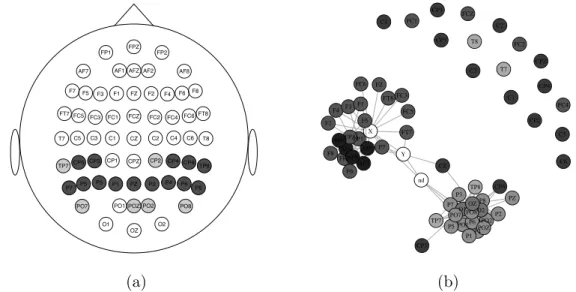
FP1 FP2 F7 F8 AF1 AF2 FZ F4 F3 FC6 FC5 FC2 FC1 T8 T7 CZ C3 C4 CP5 CP6 CP1 CP2 P3 P4 PZ P8 P7 PO2 PO1 O2 O1 X AF7 AF8 F5 F6 FT7 FT8 FPZ FC4 FC3 C6 C5 F2 F1 TP8 TP7 AFZ CP3 CP4 P5 P6 C1 C2 PO7 PO8 FCZ POZ OZ P2 P1 CPZ nd Y (a) (b)

Figure 2.6: (a) An EEG cap based on the fitted model using (λ1, λ2) = (0.15,5.66). Dark

grey channels had at least twenty time points estimated to have nonzero mean differences; light grey channels had less than twenty but greater than zero, whereas white channels had no nonzero mean differences. (b) The Gaussian precision graphical model corresponding to ˆ∆. Different shades of grey correspond to different regions of the EEG channels; white channels are those that do not appear on the EEG cap image.

complete dataset. We used the tuning parameter pair (λ1, λ2) = (0.15,5.66), which had

leave-one-out classification accuracy of 98 out of 122. The estimated mean difference, dis-played as a heatmap in Figure 2.5(b), had 15466 of 16384 entries equal to zero.

Our fitted model can be used to easily identify which channels and time points have nonzero mean differences. We estimated only 22 of the 64 channels to have at least one time point where the mean differences were nonzero, only 16 of which had at least 20 nonzero time points. Inspecting the estimated mean differences displayed in Figure 2.5, it seems that the majority of activity that distinguishes between the alcoholic and control subjects takes place between the 52nd and 115th time points. We used the R package eegkit (Helwig, 2015) to display which channels had nonzero mean differences in Figure 2.5a. Our method does not explicitly use the spatial structure of channels in estimation, yet it recovered a set of important channels which have a natural arrangement in space.

(40)

2.6. Extensions 26

ˆ

∆ had 3676 of 4032 off-diagonals equal to zero. Our estimate ˆ∆ can be interpreted in terms of a Gaussian precision graphical model corresponding to the conditional dependence struc-ture of the channels. We display the graphical model corresponding to ˆ∆ in Figure 2.6(b). The graph structure corresponds to the spatial arrangement of channels displayed in Fig-ure 2.6(a) – a result also observed by Zhou (2014).

2.6 Extensions

Our method naturally extends to the quadratic discriminant analysis model, where one assumes

vec(X|Y =j)∼Nrc{vec (µ∗j),Σ∗j},

where Σ∗j ∈S+rcis the covariance matrix for thejth class for allj∈ J. To generalize (2.2), one can assume either (i) Σ∗j = ∆∗j⊗Φ∗j, (ii) Σ∗j = ∆∗j ⊗Φ∗, and (iii) Σ∗j = ∆∗⊗Φ∗j, where under (ii) and (iii), only one of the two component precision matrices are unique to each response category. Our algorithms can be easily modified to accommodate (i),(ii), or (iii).

The assumption (2.2) and estimator (2.3) can be generalized to cases where the predictor is a multidimensional array of order three or more, such as in fMRI or video data. In this case, where xi ∈Rd1×···×dq, we can generalize the assumption (2.2) to the matrix Σ∗ ∈SK+

whereK =Qq

i=1di so that

Σ−∗1= Ξ1⊗ · · · ⊗Ξq, (2.14)

where Ξl ∈ S+dl for l = 1, . . . , q. Under (2.14), (2.1) becomes the array-normal distribu-tion (Hoff, 2011; Manceur and Dutilleul, 2013). Algorithm 1 can be generalized to this setting using the same arguments as in Section 2.3. In particular, our alternating minimiza-tion algorithm could be applied by replacing the matrix product in the right hand side of (2.11) with a tensor product. Special computational considerations may be necessary when max{d1, . . . , dq}is large. For instance, it may be better to approximate (2.3) in two steps;

(41)

2.6. Extensions 27

the first step would estimate the covariance parameters withµj fixed at ¯xj forj= 1, . . . , J, and the second step would estimate µ∗ using (2.7) with the precision matrix components fixed at their estimates.

(42)

Chapter 3

Indirect multivariate response

linear regression

3.1 Introduction

Some statistical applications require the modeling of a multivariate response. Let yi ∈Rq be the measurement of the q-variate response for the ith subject and let xi ∈ Rp be the nonrandom values of the p predictors for the ith subject (i= 1, . . . , n). The multivariate response linear regression model assumes thatyi is a realization of the random vector

Yi =µ∗+βT∗xi+εi, i= 1, . . . , n, (3.1)

where µ∗ ∈ Rq is the unknown intercept, β∗ is the unknown p by q regression coefficient matrix, andε1, . . . , εnare independent copies of a mean zero random vector with covariance matrix Σ∗E.

The ordinary least squares estimator of β∗ is ˆ

βOLS= arg min β∈Rp×q

kY−Xβk2F, (3.2)

wherek · kF is the Frobenius norm,Rp×q is the set of real valued pby q matrices, Yis the n by q matrix with ith row (Yi−n−1Pin=1Yi)T, and X is then by p matrix with ith row (xi−n−1Pn_i₌₁xi)T (i = 1, ..., n). It is well known that ˆβOLS is the maximum likelihood

(43)

3.2. A new class of indirect estimators of β∗ 29 estimator ofβ∗ when ε1, . . . , εnare independent and identically distributed Nq(0,Σ∗E) and the corresponding maximum likelihood estimator of Σ−_∗_E1 exists.

Many shrinkage estimators of β∗ have been proposed by penalizing the optimization in (3.2). Some simultaneously estimate β∗ and remove irrelevant predictors (Turlach et al., 2005; Obozinski et al., 2010; Peng et al., 2010). Others encourage an estimator of reduced rank (Yuan et al., 2007; Chen and Huang, 2012).

Under the restriction thatε1, . . . , εnare independent and identically distributed Nq(0,Σ∗E), shrinkage estimators of β∗ that penalize or constrain the minimization of the negative log-likelihood have been proposed. These methods simultaneously estimate β∗ and Σ−_∗_E1. Ex-amples include maximum likelihood reduced-rank regression (Izenman, 1975; Reinsel and Velu, 1998), envelope models (Cook et al., 2010; Su and Cook, 2011, 2012, 2013), and mul-tivariate regression with covariance estimation (Rothman et al., 2010; Lee and Liu, 2012; Bhadra and Mallick, 2013).

To fit (3.1) with these shrinkage estimators, one exploits explicit assumptions about β∗ that may be unreasonable in some applications. As an alternative, we propose an indirect method to fit (3.1) without such assumptions. We instead assume that response and pre-dictors have a joint multivariate normal distribution and we employ shrinkage estimators of the parameters of the conditional distribution of the predictors given the response. Our method provides alternative indirect estimators ofβ∗, which may be suitable when existing shrinkage estimators are inadequate. In the very challenging case when p is large and β∗ is not sparse, one of our proposed indirect estimators can predict well and be interpreted easily.

3.2 A new class of indirect estimators of

β

∗

3.2.1 Class definition

We assume that the measured predictor and response pairs (x1, y1), . . . ,(xn, yn) are a re-alization of n independent copies of (X, Y), where (XT, YT)T ∼ Np+q(µ∗,Σ∗). We also assume that Σ∗ is positive definite. Define the marginal parameters through the following

(44)

3.2. A new class of indirect estimators of β∗ 30 partitions: µ∗ =   µ∗X µ∗Y  , Σ∗ =   Σ∗XX Σ∗XY ΣT_∗_XY Σ∗Y Y  .

Our goal is to estimate the multivariate regression coefficient matrix β∗ = Σ−_∗_XX1 Σ∗XY in the forward regression model

Y |X=x∼Nq

µ∗Y +β∗T(x−µ∗X),Σ∗E ,

without assuming that β∗ is sparse or that kβ∗k2_F is small. To do this we will estimate the inverse regression’s coefficient matrix η∗ = Σ−∗Y Y1 ΣT∗XY and the inverse regression’s error precision matrix ∆−_∗1 in the inverse regression model

X |Y =y∼Np

µ∗X +η∗T(y−µ∗Y),∆∗ .

We connect the parameters of the inverse regression model toβ∗ with the following propo-sition, which we prove in Appendix A.1.

Proposition 1

If Σ∗ is positive definite, then

β∗ = ∆−∗1ηT∗ Σ−∗Y Y1 +η∗∆

−1

∗ ηT∗

−1

. (3.3)

This result leads us to propose a class of estimators ofβ∗, ˆ

β = ˆ∆−1ηˆT( ˆΣ−_{Y Y}1 + ˆη∆ˆ−1ηˆT)−1, (3.4) where ˆη, ˆ∆, and ˆΣY Y are user-selected estimators of η∗, ∆∗, and Σ∗Y Y. Ifn > p+q+ 1 and the ordinary sample estimators are used for ˆη, ˆ∆ and ˆΣY Y, then ˆβ is equivalent to ˆβOLS.

We propose to use shrinkage estimators of η∗, ∆−∗1, and Σ−∗Y Y1 in (3.4). This gives us the potential to indirectly fit an unparsimonious forward regression model by fitting a parsimonious inverse regression model. For example,η∗ could have only one nonzero entry

(45)

3.3. Asymptotic analysis 31

and all entries in β∗ could be nonzero. Conveniently, entries in η∗ can be interpreted like entries in β∗ are by reversing the roles of the predictors and responses. To fit the inverse regression model, we could use any of the forward regression shrinkage estimators discussed in Section 3.1.

3.2.2 Related work

Lee and Liu (2012) proposed an estimator of β∗ that also exploits the assumption that (XT_{, Y}T₎T _{is multivariate normal; however, unlike our approach which makes no explicit}

assumptions about β∗, they assume that both Σ−∗1 and β∗ are sparse.

Modeling the inverse regression is a well-known idea in multivariate analysis. For ex-ample, whenY is categorical, quadratic discriminant analysis treatsX|Y =y asp-variate normal. There are also many examples of modeling the inverse regression in the sufficient dimension reduction literature (Adragni and Cook, 2009).

The work most closely related to ours is Cook et al. (2013). They proposed indirect estimators of β∗ based on modeling the inverse regression in the special case when the response is univariate, i.e.,q= 1. Under our multivariate normal assumption on (XT, YT)T, Cook et al. (2013) showed that

β∗ =

1

1 + ΣT_∗_XY∆−∗1Σ∗XY/Σ∗Y Y

∆−∗1Σ∗XY, (3.5)

and proposed estimators ofβ∗by replacing Σ∗XY and Σ∗Y Y in (3.5) with their usual sample estimators, and by replacing ∆−∗1 with a shrinkage estimator. This class of estimators was designed to exploit an abundant signal rate in the forward univariate response regression when p > n.

3.3 Asymptotic analysis

We present a convergence rate bound for the indirect estimator ofβ∗ defined by (3.4). Our bound allows p and q to grow with the sample size n. In the following proposition, k · k is

(46)

3.4. Estimators in our class 32

the spectral norm andϕmin(·) is the minimum eigenvalue.

Proposition 2

Suppose that the following conditions are true: (i)Σ∗ is positive definite for allp+q; (ii) the estimatorΣˆ−_{Y Y}1 is positive definite for allq; (iii) the estimator∆ˆ−1 is positive definite for all

p; (iv) there exists a positive constant K such that ϕmin(Σ−∗Y Y1 )≥K for allq; and (v) there

exist sequences {an},{bn} and {cn} such thatkηˆ−η∗k=OP(an),k∆ˆ−1−∆∗−1k=OP(bn),

kΣˆ−_{Y Y}1 −Σ−_∗_{Y Y}1 k=OP(cn), andankη∗kk∆−∗1k+bnkη∗k2+cn→0 as n→ ∞. Then

kβˆ−β∗k=OP ankη∗k2k∆−∗1k2+bnkη∗k3k∆−∗1k+cnkη∗kk∆−∗1k

.

We prove Proposition 2 in Appendix A.1. We used the spectral norm because it is compat-ible with the convergence rate bounds established for sparse inverse covariance estimators (Rothman et al., 2008; Lam and Fan, 2009; Ravikumar et al., 2011).

If the inverse regression is parsimonious in the sense thatkη∗kandk∆−∗1kare bounded, then the bound in Proposition 2 simplifies to kβˆ−β∗k = OP(an+bn+cn). We explore finite-sample performance in Section 3.5.

3.4 Estimators in our class

3.4.1 Sparse inverse regression

We now describe an estimator of the forward regression coefficient matrix β∗ defined by (3.4) that exploits zeros in the inverse regression’s coefficient matrixη∗, zeros in the inverse regression’s error precision matrix ∆−1

∗ , and zeros in the precision matrix of the responses Σ−_∗_{Y Y}1 . We estimate η∗ with ˆ ηL1= arg min η∈_Rq×p    kX−Yηk2F + p X j=1 λj q X m=1 |ηmj|    , (3.6)

(47)

which separates into p L1-penalized least-squares regressions (Tibshirani, 1996): the first

predictor regressed on the response through the pth predictor regressed on the response. We selectλj with 5-fold cross-validation, minimizing squared prediction error totaled over the folds, in the regression of the jth predictor on the response (j= 1, . . . , p). This allows us to estimate the columns ofη∗ in parallel.

We estimate ∆−∗1 and Σ−∗Y Y1 with L1-penalized Gaussian likelihood precision matrix estimation (Yuan and Lin, 2007; Banerjee et al., 2008). Let ˆΣ−_γ,S1 be a generic version of this estimator with tuning parameterγ and inputp by p sample covariance matrixS:

ˆ Σ−_γ,S1 = arg min Ω∈_Sp₊    tr(ΩS)−log|Ω|+γX j6=k |ωjk|    , (3.7)

whereSp+is the set of symmetric and positive definitepbyp matrices. The optimization in

(3.7) was used to estimate the inverse regression’s error precision matrix in the univariate response regression methods proposed by Cook et al. (2012) and Cook et al. (2013). There are many algorithms that solve (3.7). Two good choices are the graphical lasso (Yuan, 2008; Friedman et al., 2008) and the algorithm of Hsieh et al. (2011). We select γ with 5-fold cross-validation maximizing a validation likelihood criterion (Huang et al., 2006):

ˆ γ = arg min γ∈G 5 X k=1 n tr ˆ Σ−_γ,S1 (−k)S(k) −log ˆ Σ−_γ,S1 (−k) o , (3.8)

where G is a user-selected finite subset of the non-negative real line, S(−k) is the sample

covariance matrix from the observations outside the kth fold, and S₍_k₎ is the sample co-variance matrix from the observations in thekth fold centered by the sample mean of the observations outside the kth fold. We estimate ∆−_∗1 using (3.7) with its tuning parameter selected by (3.8) and S = (X−YηˆL1)T(X−YηˆL1)/n. Similarly, we estimate Σ−∗Y Y1 using (3.7) with its tuning parameter selected by (3.8) andS =YTY/n.

(48)

3.4.2 Reduced-rank inverse regression

We propose indirect estimators of β∗ that presupposes that the inverse regression’s coeffi-cient matrix η∗ is rank-deficient. The following proposition links rank deficiency in η∗ and its estimator to β∗ and its indirect estimator.

Proposition 3

If Σ∗ is positive definite, then rank(β∗) = rank(η∗). In addition, if Σˆ−_{Y Y}1 and ∆ˆ−1 are positive definite in the indirect estimatorβˆdefined by (3.4), then rank( ˆβ) = rank(ˆη).

We propose two reduced-rank indirect estimators ofβ∗by inserting estimators ofη∗,∆−∗1, and Σ∗Y Y in (3.4). The first estimates Σ∗Y Y with YTY/n and estimates (η∗,∆−∗1) with normal likelihood reduced-rank inverse regression:

(ˆη(r),∆ˆ−1(r)) = arg min (η,Ω)∈_Rq×p_× Sp+ n−1tr (X−Yη)T(X−Yη)Ω −log det(Ω) (3.9) subject to rank(η) =r,

wherer is selected from{0, . . . ,min(p, q)}. The solution to (3.9) is available in closed form (Reinsel and Velu, 1998).

The second reduced-rank indirect estimator ofβ∗estimatesη∗with ˆη(r)defined in (3.9), estimates Σ−_∗_{Y Y}1 with (3.7) using S = YTY/n, and estimates ∆−∗1 with (3.7) using S = (X−Yηˆ(r))T(X−Yηˆ(r))/n.

The first indirect estimator is likelihood-based and the second indirect estimator exploits sparsity in Σ−_∗_{Y Y}1 and ∆−∗1. Neither estimator is defined when min(p, q)> n. In this case, which we do not address, a regularized reduced-rank estimator ofη∗ could be used instead of the estimator defined in (3.9), e.g., the factor estimation and selection estimator (Yuan et al., 2007) or the reduced-rank ridge regression estimator (Mukherjee and Zhu, 2011).

Model-based methods for high-dimensional multivariate analysis