San Jose State University
SJSU ScholarWorks
Master's Projects Master's Theses and Graduate Research
Fall 2013
Metamorphic Detection Using Singular Value
Decomposition
Ranjith Kumar Jidigam
San Jose State University
Follow this and additional works at:https://scholarworks.sjsu.edu/etd_projects Part of theComputer Sciences Commons
This Master's Project is brought to you for free and open access by the Master's Theses and Graduate Research at SJSU ScholarWorks. It has been accepted for inclusion in Master's Projects by an authorized administrator of SJSU ScholarWorks. For more information, please contact
Recommended Citation
Jidigam, Ranjith Kumar, "Metamorphic Detection Using Singular Value Decomposition" (2013).Master's Projects. 330. DOI: https://doi.org/10.31979/etd.838t-v2qr
Metamorphic Detection Using Singular Value Decomposition
A Project Presented to
The Faculty of the Department of Computer Science San Jose State University
In Partial Fulfillment
of the Requirements for the Degree Master of Science
by
Ranjith Kumar Jidigam December 2013
c
○2013
Ranjith Kumar Jidigam ALL RIGHTS RESERVED
The Designated Project Committee Approves the Project Titled
Metamorphic Detection Using Singular Value Decomposition
by
Ranjith Kumar Jidigam
APPROVED FOR THE DEPARTMENTS OF COMPUTER SCIENCE
SAN JOSE STATE UNIVERSITY
December 2013
Dr. Mark Stamp Department of Computer Science
Dr. Thomas Austin Department of Computer Science
ABSTRACT
Metamorphic Detection Using Singular Value Decomposition by Ranjith Kumar Jidigam
Metamorphic malware changes its internal structure with each infection, while maintaining its original functionality. Such malware can be difficult to detect using static techniques, since there may be no common signature across infections. In this research we apply a score based on Singular Value Decomposition (SVD) to the problem of metamorphic detection. SVD is a linear algebraic technique which is applicable to a wide range of problems, including facial recognition. Previous research has shown that a similar facial recognition technique yields good results when applied to metamorphic malware detection. We present experimental results and we analyze the effectiveness and efficiency of this SVD-based approach.
ACKNOWLEDGMENTS
I am very thankful to my advisor Dr. Mark Stamp for his continuous guidance and support throughout this project and believing me. Also I would like to thank the committee members Dr. Thomas Austin and Dr. Richard Low for monitoring the progress of the project and their valuable time.
TABLE OF CONTENTS
CHAPTER
1 Introduction . . . 1
2 Malware . . . 3
2.1 Metamorphic Techniques . . . 3
2.1.1 Garbage Code and Dead Code . . . 3
2.1.2 Instruction Substitution . . . 3
2.1.3 Instruction Reordering . . . 4
2.1.4 Register Swapping . . . 4
2.1.5 Host Code Mutation . . . 4
2.2 Metamorphic Malware . . . 4
2.2.1 G2 . . . 5
2.2.2 MPCGEN . . . 5
2.2.3 NGVCK . . . 5
2.2.4 MWOR . . . 5
2.3 Malware Detection Techniques . . . 6
2.3.1 Signature scanning and heuristics . . . 6
2.3.2 Machine Learning . . . 6
2.3.3 n-gram Analysis . . . 7
2.3.4 Code Disassembling . . . 7
2.3.5 Code Emulation . . . 7
2.3.7 Simple Substitution . . . 7
2.3.8 Structural Entropy . . . 8
3 Singular Value Decomposition and Eigenface . . . 9
3.1 Eigenvalues and Eigenvectors . . . 10
3.2 Image Detection . . . 11
3.3 Singular Value Decomposition . . . 13
4 Singular Value Decomposition for Malware . . . 15
4.1 Algorithm . . . 15
4.1.1 Training Phase . . . 15
4.1.2 Testing Phase . . . 19
5 Implementation . . . 20
5.1 Extract Raw Bytes . . . 20
5.2 Pictorial Representation of Technique . . . 21
5.3 Environment Setup . . . 22 5.4 JAMA Library . . . 23 6 Experimental Results . . . 24 6.1 Results . . . 25 6.1.1 MWOR . . . 25 6.1.2 NGVCK . . . 30 6.1.3 G2 . . . 31
6.2 Receiver Operating Characteristic (ROC) Curves . . . 31
6.3 AUC statistics . . . 37
LIST OF TABLES
1 Software and Hardware configuration . . . 23
2 Malware Datasets . . . 24
3 Benign Datasets . . . 25
4 NGVCK and G2 AUC . . . 32
5 MWOR AUC values . . . 33
6 NGVCK and G2 AUC values using two eigenvectors . . . 37
7 MWOR AUC values using two Eigenvectors . . . 38
8 NGVCK and G2 AUC values using three Eigenvectors . . . 38
9 MWOR AUC values using three Eigenvectors . . . 39
10 Turboc scores against different compiler datasets . . . 39
11 Clang scores against different compiler datasets . . . 40
12 Mingw scores against different compiler datasets . . . 40
LIST OF FIGURES
1 Eigenvalue and Eigenvector . . . 10
2 Original Images . . . 11
3 Eigenfaces of the Original Images . . . 12
4 Projection of known and unknown images into the eigenspace . . . . 13
5 Matrix transformation using SVD . . . 14
6 Text Section Bytes . . . 21
7 Implementation . . . 22
8 Scatter Plot for MWOR_1.0 . . . 26
9 Scatter Plot for MWOR_1.5 . . . 27
10 Scatter Plot for MWOR_2.0 . . . 27
11 Scatter Plot for MWOR_2.5 . . . 28
12 Scatter Plot for MWOR_3.0 . . . 28
13 Scatter Plot for MWOR_4.0 . . . 29
14 Scatter Plot for NGVCK . . . 30
15 Scatter Plot for G2 . . . 31
16 ROC for Mwor_1.0 . . . 33
17 ROC for Mwor_3.0 . . . 34
18 ROC for Mwor_4.0 . . . 34
19 ROC for NGVCK . . . 35
20 ROC for NGVCK . . . 36
CHAPTER 1 Introduction
Malware is a major threat to the cyber space. It is estimated that annually the losses incurred by computer malware is $114 billion worldwide [17]. With the ad-vancement in technology, usage of gadgets etc., malware attacks have been increasing rapidly. Malware is a piece of software payload that injects in to the host file causing denial of service, stealing confidential information etc.,. With the generation of new malware everyday there is a mandate need for efficient detection techniques [11].
Metamorphic malware mutates so that every infection is different. Different morphing techniques like garbage code insertion, register swap, instruction reordering etc., are implemented to generate malware to achieve code obfuscation. Malware writers have become so intelligent in morphing malware that is hard to detect. Many reasons like software bugs, unawarness among naive internet users etc., are few reasons that provide entry points for malware into the cyber space [10].
The base for this paper is from a facial recognition technique Eigenfaces [29]. In this paper we have extended the previous work done on malware detection using eigenvalue analysis technique [22]. We modified the implementation by using Singular Value Decomposition (SVD) [13, 24]. SVD is applied on highly metamorphic malware families that have evaded detection by statistical approaches. In this technique we pre-processed the malware executables to extract the raw bytes from the text section. Then we implemented SVD to determine the singular space which represents the cor-relation among the malware files. Malware test dataset and benign files are projected on to this space to determine if they are close to the training malware dataset. We
have done experiments on highly metamorphic malware and got good results.
The paper is organized as follows. Chapter 2 describes about malware genera-tion, different types of malware and malware detection techniques. Chapter 3 tells about the eigenfaces and eigenvectors in facial recognition. Implementation of SVD technique on metamorphic malware is described in Chapter 4. Test setup, software and hardware requirements and JAMA(Java Matrix) API are briefed in Chapter 5. Chapter 6 shows the experimental results and conclusion in Chapter 7.
CHAPTER 2 Malware
In this chapter we provide a brief background information that is relevant to the technique implemented. First we begin with malware morphing techniques and then about malware types.
2.1 Metamorphic Techniques
Malware is generated by performing swapping, insertion, substitution operations on assembly code instructions. The amount of morphing determines the strength of the malware. Following is the description of morphing techniques.
2.1.1 Garbage Code and Dead Code
Garbage code does not have any functionality. It is called as do nothing code. The program functionality does not change with garbage code insertion. For example the instruction NOP does not have any functionality. On the other hand dead code is the code which is never reached. Both these morphing strategies can be used to defend against signature based detection approaches and are effective defenses against statistical based detection techniques [7].
2.1.2 Instruction Substitution
In this morphing technique an instruction is replaced with its equivalent instruc-tion by keeping the funcinstruc-tionality the same. Registers are used interchangeably in this technique [32]. This acts as a strong defense against signature based detection and is used in metamorphic generators.
2.1.3 Instruction Reordering
As the name suggests this technique works by shuffling the blocks and modules in an malware executable to generate a new infection. Inserting jump instructions in between modules by keeping the functionality the same is the main process im-plemented in this. As the blocks are shuffled this technique is an effective defense against signature based detection strategies [7] and also against structural detection approaches [25].
2.1.4 Register Swapping
In register swapping technique the virus instruction operands are stored in dif-ferent registers for each new infection. Wildcard pattern matching would detect this technique.
2.1.5 Host Code Mutation
Some malware infections like Win95/Bistro morph their code as well as the orig-inal code of host file into which they are inserted [15]. It is too difficult to implement this technique. As the host code itself mutates it is hard to detect this malware.
2.2 Metamorphic Malware
Malware is generated to achieve code obfuscation. We mentioned different mal-ware generation techniques in previous section. We describe about different malmal-ware families [3] in this section.
2.2.1 G2
G2 malware family is called as second generation malware. It is modestly meta-morphic malware [31]. It is generated by using instruction substitution morphing technique.
2.2.2 MPCGEN
Mass produced code generation kit malware family is mild. When compared with randomly selected benign code this malware family exhibits more similarity between each infection [4, 31].
2.2.3 NGVCK
The next generation virus construction kit uses garbage code insertion, register swapping, code reordering techniques to generate sufficiently morphed malware [30]. This malware is written in visual basic and it generates 32 bit executable files. This malware family evades signature based detection techniques but can be detected using statistical approach [21, 28, 31].
2.2.4 MWOR
For research purposes MWOR malware has been created. Morphing engine is present along with the worm. Morphing is done by instruction substitution and garbage code insertion. The morphing is on par with NGVCK and hence this worm evades signature based detection. The flexibility with this worm is user can specify the level of morphing and dead code from non-virus files is inserted. Morphed code is indistinguishable from benign code at sufficient padding ratio causing statistical detection techniques to fail [26]. For the experiments we used malware with padding
ration ranging from 0.5 to 4.0. Padding ratio 0.5 represents that dead code equivalent to 50% of the actual worm size has been inserted. High padding ratios implements that more code from linux benign files has been inserted in to the virus replicate.
2.3 Malware Detection Techniques
A number of malware detection techniques [11, 16] have been proposed in the recent past but with the growth in the number of cyber security attacks there is a mandate need for fast and efficient malware detection techniques.
The paper tells about current malware detection techniques. Based on the com-parison between different detection techniques and the problems with these techniques in identifying modern malware the paper proposed the need for new malware detction techniques. Malware is detected using following approaches.
2.3.1 Signature scanning and heuristics
Few malware families are generated just by instruction swapping or instruction substitution methods, such malware can be detected by just looking for a common signature. Sometimes heuristics can be applied to detect poorly morphed malware.
2.3.2 Machine Learning
Machine Learning is implemented across a lot of domains in computer industry. For malware detection Hidden Markov Model (HMM) [2, 20, 26, 27] is a famous technique that is used to learn about the malware data and result some information. Opcode sequences of malware executable are trained using HMM. The trained HMM is then used to score malware test and benign files. The highly morphed virus family NGVCK are easily detected using this HMM technique.
2.3.3 n-gram Analysis
In n-gram Analysis technique overlapping sequence of n bytes of malware exe-cutable is considered and frequency table is generated [31]. Benign and virus files are evaluated to calculate frequencies of overlapping bytes and then is scored against the frequency table built for malware family files. This technique also detects NGVCK malware effectively.
2.3.4 Code Disassembling
A malware file is diassembled and is analyzed to identify the garbage instructions. This model when used with Hidden Markov Model gives efficient results.
2.3.5 Code Emulation
Virus files are executed in a Virtual Machine. The exectuion is carefully moni-tored to identify the virus payload.
2.3.6 Opcode Graph Analysis
Graphs are constructed for opcode digraph frequencies. Then a test file frequen-cies are compared against this trained frequenfrequen-cies. A detailed experiment is given in paper [21]. This technique detects MWOR metamorphic worms effectively.
2.3.7 Simple Substitution
An experiment using simple substitution is analyzed in paper [23]. In this, all the opcode digraph statistics of malware family are gathered and when we want to classify a file, we collect its opcodes and then simple substitution attack is applied with the malware family statistics as language statistics. A high score implies that
the file can be transformed using language statistics to match a malware family file.
2.3.8 Structural Entropy
Wavelet analysis is used to segment files based on varying entropy levels. These segments are then compared used Levenshtein distance to computer a score. This technique is not costly as it is applied on binary files. The technique is more analyzed in paper [5, 25]. The results shows that MWOR worms are detected correctly.
CHAPTER 3
Singular Value Decomposition and Eigenface
A facial recognition technique Eigenfaces for recognition is the basis for this implementaion. Similar technique is implemented on the malware files to identify the correlation between the same.
Facial recognition is an important field of study as it has applications across various domains like detecting criminals, digital animation, identifying the owner of the gadgets, identifying the employees etc., Face recognition is a challenging task as there are many features to consider like ear, nose, eyes etc., Also external features like light focus in the image, different face expressions of the person, difference in age etc., are also few challenging things to determine the relation among the images. All the features in a face are represented in three dimensional vectors and it is hard to implement the recognition technique. But a flat upright image is represented in two dimensional vector (pixel values). This consideration helps in implementing facial recognition and also to get accurate results.
A facial image can be decomposed further into small characteristic feature images called eigenfaces. These eigenfaces represent the significant features of the image. The space spanned by these eigenfaces is called facespace. When a new image has to be tested to see if it resembles any of the trained facial image, it is projected on to this face space and a score is calculated to determine how relavant the test image is to the trained facial image. This technique is a kind of clustering technique which depicts the relation among the input images.
3.1 Eigenvalues and Eigenvectors
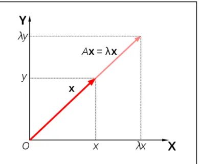
Eigen means unique or belonging [9]. Eigenvectors are also called as characteristic vectors. In linear algebra, if a non-zero vector 𝑥 satisfies the following equation for a square matrix 𝐴, then 𝑥 is called an eigenvector of 𝐴 and 𝜆 is called the eigenvalue associated with the eigenvector 𝑥. The equation
𝐴𝑥=𝜆𝑥
represents the eigenvector 𝑥 and 𝜆 , the eigenvalue is a scalar.
Figure 1: Eigenvalue and Eigenvector
Eigenvector and Eigenvalue are represented in the Figure 1. Matrix 𝐴 contains data points of 𝑛 files aligned in 𝑛 columns. The variation among all these data points is represented by covariance matrix. Eigenvectors helps in quantifying the similarity between the various data points. So eigenvectors and eigenvalues for this covariance matrix are calculated and when these eigenvectors are projected into space they enclose an area called as eigenspace. More the eigenvalue, more important is its
corresponding eigenvector in contributing to the variance among the data points of
𝑛 files. In facial recognition technique these 𝑛 files corresponds to 𝑛 different images and data points represents the pixel values.
3.2 Image Detection
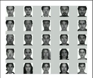
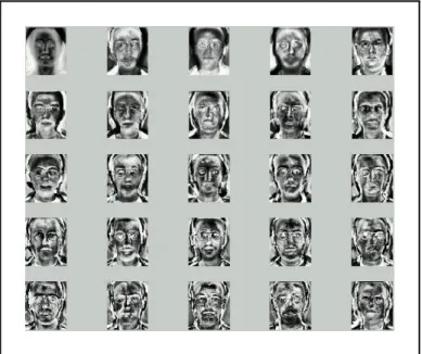
In the image detection technique eigenvectors of the covariance matrix are de-termined [8]. These eigenvectors when projected into the space they enclose an area called face space. When we project a known image on to this face space we can re-construct the original image in terms of eigenvectors associated with weights. Not all eigenvectors contributes to the original image. In facial recognition technique after constructing a column vector with pixels of each image we subtract the mean pixel value all the training input images at that position from the actual pixel value of all the images. Figure 2 represents the original face images and their ghost images in Figure 3 when projected on to this face space.
Figure 2 contains the original face images that are used for training. The equiv-alent eigenfaces are represented in Figure 3.
Figure 3: Eigenfaces of the Original Images
Each eigenvector has corresponding weight associated with it. When we sum up all the eigenvectors along with their weights we can reconstruct the original im-age. An image 𝑀 containing 𝑚 ×𝑛 pixels can be represented as a vector 𝑉. Let
𝐸1, 𝐸2, 𝐸3, . . . , 𝐸𝑛 are the eigenvectors constructed from a set of images where image
𝑀 is one among them. Now when we project vector 𝑉 on to this facespace con-structed by 𝐸1, 𝐸2, 𝐸3, . . . , 𝐸𝑛 we can construct the original image. Now the sum of
eigenvectors and their corresponding weights gives the vector
𝑉 =𝑤1𝐸1+𝑤2𝐸2 +𝑤3𝐸3+. . .+𝑤𝑛𝐸𝑛
where 𝑤1, 𝑤2, 𝑤3, . . . , 𝑤𝑛 represents the weights associated with the eigenvectors
𝐸1, 𝐸2, 𝐸3, . . . , 𝐸𝑛. Weights of known and unknown images are compared against
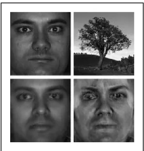
When a known image is projected on to the eigenspace we can reconstruct the original image and when an unknown image is projected on to the eigenspace we cannot construct the original image. The Figure 4 represents the projection of known and unknown images on to the eigenspace. This Figure 4 is taken from CMU PIE database of images.
Figure 4: Projection of known and unknown images into the eigenspace
3.3 Singular Value Decomposition
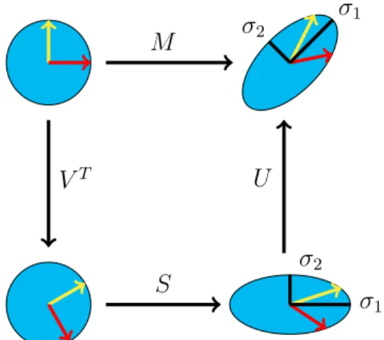
Singular Value Decomposition [24] is a factorization of a real matrix. The basic idea behind SVD is taking high variable set of data points and reducing it to a lower dimensions set that better exposes the substructure of the original data more clearly by ordering the lower dimensional data from most variance to the least. SVD of a real 𝑚*𝑛 matrix 𝐴 is a factorization of the form
𝐴=𝑈 𝑆𝑉𝑇
Matrix 𝑈 contains left singular vectors of 𝐴 which are generated by calculating the eigenvectors of 𝐴𝐴𝑇. Matrix 𝑉 contains right singular vectors of 𝐴, generated by
calculating eigenvectors of 𝐴𝑇𝐴. Matrix 𝑆 is a diagonal matrix with square root of
eigenvalues common to the matrices 𝑈 and 𝑉. 𝑈 𝑈𝑇 and 𝑉𝑇𝑉 are identity matrices.
Here the eigenvectors of the matrix 𝑈 are normalized by dividing each eigenvector with square root of its corresponding eigenvalue. That is why the eigenvectors of the matrix 𝑈 are called as singularvectors.
The matrix𝑈 contains eigenvectors sorted according to the singular values in the matrix 𝐴. Figure 5 represents the Singular Value Decomposition on a 𝑚×𝑛 matrix
𝐴. 𝜎1 𝜎2 𝜎1 𝜎2 𝑀 𝑆 𝑉𝑇 𝑈
CHAPTER 4
Singular Value Decomposition for Malware
We discussed about Singular Value Decomposition and its implementation in Image Recognition in the previous Chapter 3. Similar technique was implemented in the paper Eigenviruses [12]. This serves as the basis for our implementation. In this Chapter we describe about the SVD algorithm implemented in training and testing malware files. The goal of the training phase is to determine the weights of the training input files by projecting them on to the eigenspace. In the testing phase we project the virus and benign test files on to this eigenspace to determine their weights and then calculate the euclidean distance between the weights of the training files and test files.
SVD is represented as 𝐴 =𝑈 𝑆𝑉𝑇. Eigenspace is determined by projecting the
eigenvectors of the covariance matrix 𝐴𝐴𝑇, which are represented by the matrix 𝑈.
Matrix𝑆 is a diagonal matrix with square root of eigenvalues common to the matrices
𝑈 and 𝑉. We are considering singular vectors of the matrix 𝑈 for calculating the weights of training and testing files.
4.1 Algorithm
The training and testing phases follow a step by step process. The algorithm implemented in these phases is described below.
4.1.1 Training Phase
In the training phase first extract the raw bytes from the text or code sections of all the input training files and construct a column vector for each file. Then
deter-mine the eigenvectors of the covariance matrix. These covariance matrix eigenvectors represents the eigenspace. We do not consider all the eigenvectors for generating the eigenspace as vectors with low eigenvalue are less important. Then we project each input training file on to this eigenspace to get set of weights. Implementation of this phase is explained below.
1. Acquire a set of 𝑀 virus replicates of a particular malware family 2. Extract raw bytes from the text or code section of each virus replicate
3. Construct a matrix 𝐴 = [Φ1,Φ2,Φ3, . . . ,Φ𝑀] with vectors where each vector
represents the raw bytes of a particular virus replicate arranged in a column. Let us say that the maximum number of bytes in a particular replicate among all replicates are𝑁, then the number of rows in matrix𝐴 will be𝑁. Append zeros to other columns which has less than 𝑁 bytes. In case of image recognition we subtract the mean image (obtained by taking average of pixel values of all the training images) from each image vector. However in case of malware detection we are ignoring this as subtracting byte values does not make any sense. 4. Now in order to identify the variance between different malware replicates find
the eigenvectors of the covariance matrix𝐶.
𝐶 = 1 𝑀 𝑀 ∑︁ 𝑖=1 Φ𝑖Φ𝑖𝑇 (1) =𝐴𝐴𝑇
where 𝑀 = number of files
5. Matrix 𝐴 dimensions are 𝑁 × 𝑀. Covariance matrix 𝐶 dimensions will be
general computing power and moreover all the eigenvectors are not important. So alternatively we can calculate eigenvectors from another matrix 𝐿 which is generated from𝐴𝑇𝐴. The dimensions of𝐿are𝑀×𝑀. Let𝜈
𝑖be the eigenvector
of the matrix𝐿. Then the following equation gives the eigenvectors of the matrix
𝐿.
𝐿𝑣𝑖 =𝜆𝑖𝑣𝑖 (2)
𝐴𝑇𝐴𝑣𝑖 =𝜆𝑖𝑣𝑖
where 𝜆𝑖 is the eigenvalue.
Multiplying both sides of the above equation with 𝐴 gives us the eigenvectors of the covariance matrix 𝐶.
𝐴𝐴𝑇𝐴𝑣𝑖 =𝜆𝑖𝐴𝑣𝑖 (3)
𝑖.𝑒., 𝐶𝐴𝑣𝑖 =𝜆𝑖𝐴𝑣𝑖
𝐴𝑣𝑖 is the eigenvector of the covariance matrix𝐶. If 𝑣 is the set of eigenvectors
of 𝐿 then 𝐴𝑣 is the set of eigenvectors of𝐶. where𝑣 = 𝑣1, 𝑣2, . . . , 𝑣𝑖.
This reduced output of covariance matrix is called as Reduced Singular Value Decomposition. Therefore the multiplication of matrix 𝐴with the eigenvectors matrix 𝑣 gives the eigenvectors of covariance matrix 𝐶. We can represent it as 𝑢=𝐴𝑣. The eigenvectors in the matrix 𝑢 are normalized by dividing each eigenvector with square root of its corresponding eigenvalue.
6. Sort the eigenvectors 𝑢 according to their associated eigenvalue in descending order. The higher the eigenvalue the more important is its corresponding eigen-vector.
7. We consider only 𝑀‘ eigenvectors out of 𝑀, where 𝑀‘< 𝑀. We project these eigenvectors in to the space and the space spanned by these vectors is called eigenspace. As eigenvectors with small eigenvalue does not contribute much to the eigenspace. We determine the value of 𝑀‘ heuristically by conducting experiments for different value of𝑀‘.
8. We can construct the original virus replicate from these𝑀‘vectors when added with their corresponding weights. Lets us say for a virus file “𝜑” in the training set with eigenvectors𝑢1, 𝑢2, 𝑢3, . . . , 𝑢𝑛 we can get back the virus files as below
𝜑=𝑤1*𝑢1+𝑤2*𝑢2+. . .+𝑤𝑀‘*𝑢𝑀‘ (4) 𝜑 = 𝑀‘ ∑︁ 𝑖=1 𝑤𝑖𝑢𝑖 (5)
where 𝑀‘ represents important eigenvectors.
Then we can determine weights of a particular virus replicate ’𝜑’ as follows
𝑤𝑖 = 𝑀‘
∑︁
𝑖=1
𝑢𝑖𝑇𝜑 (6)
We represent the set of weights of a virus replicate𝜑𝑖 as
Ω𝑇𝑖 = [𝑤1, 𝑤2, . . . , 𝑤𝑀‘] (7)
Similarly we project all the training dataset virus replicates on to this eigenspace and determine their corresponding weight vectors.
9. The weights of all the virus replicates together are represented as ∆.
∆ = [Ω1,Ω2, . . . ,Ω𝑀‘] (8)
The set of weights of all the virus replicates after projecting them on to the eigenspace is the output of training phase.
4.1.2 Testing Phase
In this phase we construct a column vector for each test file and project on to this eigenspace generated in the previous section. For training phase any file with total bytes less than𝑁 is appended with zeros and files with bytes more than𝑁 bytes are chopped off from the bottom to make the column vector size to𝑁 rows. Once we determine the weights of test file we compare these weights against weight vector of each virus replicate generated in the training phase. We calculate euclidean distance between these weight vectors. If the test file is close to the training data set virus replicates then we get a score below the predetermined threshold score. Here are the steps in the training phase
1. Project the test file 𝜑𝑛 on to the eigenspace or singularspace to determine its
weights. 𝑤𝑖 = 𝑀 ∑︁ 𝑖=1 𝑢𝑖𝑇𝜑𝑛 Ω𝑇𝑛 = [𝑤1, 𝑤2, . . . , 𝑤𝑀‘] (9)
2. Now calculate the euclidean distance between this vectorΩ𝑛and weight vectors generated in the training phase. IfΩ𝑖 is the weight vector of a training file then the euclidean distance is calculated as below.
𝜖𝑖 =
√︁
(𝜔2
1 −𝜌21) + (𝜔22−𝜌22) +. . .+ (𝜔2𝑀 −𝜌2𝑀)
where𝜔 represents weights of the training files and𝜌represents weights of test replicate.
3. First, few virus replicates that are close to the training data set are tested to determine a threshold score. Then we test benign files by calculating the euclidean score and checking if is below or above the threshold.
CHAPTER 5 Implementation
In this chapter we describe about preprocessing the input files that includes extracting raw bytes from the text or code section, diagramatic representation of the technique, the environment set up and JAMA linear algebra library.
5.1 Extract Raw Bytes
The code or text section code contains the actual application logic in any ex-ecutable file. In case of malware replicates this is the place where virus payload instructions are present. So we extract text section bytes and then construct our input training matrix. The number of bytes varies across the different malware fami-lies and also benign files. We converted these byte values to their equivalent decimal values and constructed the input training matrix as SVD can be implemented only on integer or float data points. The Singular Vectors are already normalized in the actual implementation of SVD.
Figure 6 represents the code section instructions of a highly morphed malware replicate NGVCK. We can clearly see that the middle colum represents the byte values of the correpsonding instructions in the third column. We constructed a column vector for each malware replicate by arranging the byte values in a sequnce. For example in the Figure 6 the sequence of bytes in the input training vector is c1, e0, 1e, e8, 00 and so on. Corresponding decimal values of thes bytes are inserted into the input matrix while implementing the SVD.
Figure 6: Text Section Bytes
5.2 Pictorial Representation of Technique
We extract raw bytes from the text section of all the training set malware files and construct a training input matrix 𝐴 [19]. If there are 𝑀 training files and the maximum number of bytes among all the files is 𝑁 then the matrix 𝐴 dimensions are 𝑁 *𝑀. We then pass this huge matrix to the JAMA API developed for Java to calculate the Singular Values and Singular Vectors of the covariance matrix. Once we obtain the Singular Vectors we calculate the weights of the training files by projecting them on to the singular space generated.
Similarly we project test files on to the singular space and determine their weights. Then we compute the euclidean distance between the weights of each test file and weights of all the training files. Here is the diagramatic representation of the whole process
Figure 7: Implementation
It is obvious from the Figure 7 that raw bytes are extracted from both test and train files. To generate eigenvalues and vectors we consider bytes from only the train files. Once these eigenvectors are determined the test and train files are projected on to this space to determine their weights between which euclidean distance is computed. First we test malware files agains this training dataset and we then determine a threshold. Later we calculate euclidean scores for benign files. Ideally the values for benign files should be above this threshold score.
It is not very easy to find the test files with exact size of the training files. So instead we considered files with more instruction bytes and then chopped off the bytes from the end. For the smaller files with less instructions we append zeroes. We tested files with more bytes than the maximum number of bytes in the input training files.
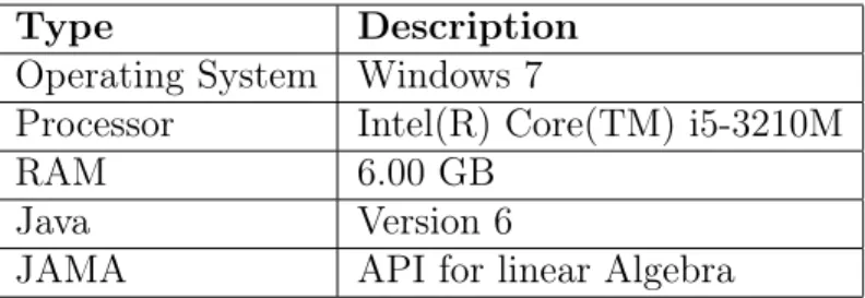
5.3 Environment Setup
Table 1: Software and Hardware configuration
Type Description
Operating System Windows 7
Processor Intel(R) Core(TM) i5-3210M
RAM 6.00 GB
Java Version 6
JAMA API for linear Algebra
In general it is not feasible to calculate the singular vectors for all the input training vectors as the covariance matrix is huge. Instead we calculate the eigenvec-tors for the reduced covariance matrix and then calculate singular veceigenvec-tors. Detailed implementation of this is explained in previous Chapter 3. SVD technique is imple-mented on the configuration in Table 1. The technique is quick enough in calculating the scores.
5.4 JAMA Library
JAMA [14] stands for Java Matrix. It is a linear algebra package that is devel-oped by National Institute of Standards and Technology(NIST). Modules in this API calculates the eigenvalues and eigenvectors as accurately as Matlab. Using this API we can solve complex matrix operations quickly. We used Jama-1.0.3.jar file for Java in calculating the singular values and vectors.
CHAPTER 6 Experimental Results
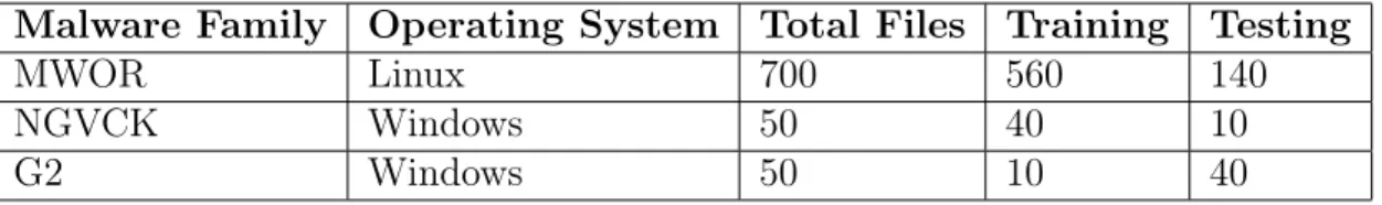
We carried our testing on different malware families and benign files as listed in Tables 2 and 3. We used the malware files efficiently by performing five fold cross technique i.e., by randomly shuffling the malware train and test datasets. For all the rounds we used 80% files for training and remaining 20% files for testing. For all the five folds the train and test files differs but the benign test files remain same. Table 2 tells about the number of virus replicates that are used for training and testing purposes.
Table 2: Malware Datasets
Malware Family Operating System Total Files Training Testing
MWOR Linux 700 560 140
NGVCK Windows 50 40 10
G2 Windows 50 10 40
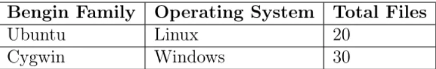
There are windows and linux based malware families in our training datasets. G2 malwar families are less morphed when compared with MWOR and NGVCK so we noticed that the technique could find better correlation between the data points for just ten training files in case of G2. The results section for G2 justifies this assumption. If the malware files are highly morphed then we consider more replicates of that malware family for training phase. For the benign test files we took files from both the operating systems and tested them against the type of malware. Table 3 describes the number of windows and linux files used for testing.
Table 3: Benign Datasets
Bengin Family Operating System Total Files
Ubuntu Linux 20
Cygwin Windows 30
6.1 Results
Following sub-sections shows the scores obtained for malware and benign files against the training dataset. These scores are obtained by calculating the euclidean distance between weights of the test files and train files after projecting them on to eigenspace.
6.1.1 MWOR
MWOR is highly metamorphic malware generated in a academic thesis [26]. The paper tells about experiments carried out in generating different padding ratio malware datasets. This malware replicates are linux based. The padding ratio at the end indicates that the percentage of dead code that has been inserted in to the malware replicates. For example MWOR_0.5 indicates that 50% of dead code has been inserted into the malware replicate, MWOR_4.0 says that 400% of malware replicates has dead code. This dead code is taken from 20 linux benign files.
From the experiments carried out on all the padding ratios we observed that a proper threshold can be set for the scores obtained for padding ratios upto 2.0. For padding ratios after 2.0, it is little hard to obtain a clear threshold between benign and malware test dataset scores. The reason for this is as the padding ratio increases most of the instructions in the malware replicates matches the instrutions in the
benign linux files.
Figure 8 represents the scores obtained for MWOR_1.0 virus replicates against the linux files.
Figure 8: Scatter Plot for MWOR_1.0
From the Figure 9 we can interpret that all the malware and benign files are classified properly. The AUC and ROC values mentioned in the below sections tells more about the false and true positives obtained for this dataset.
Figure 9: Scatter Plot for MWOR_1.5
The scatter plot for the MWO_1.5 also gives a proper threshold. We can clearly distinguish the scores of the benign linux files and malware replicate files. Out of the 20 files we tested against this padding ratio files we observed 0% false positives and 0% false positives. Scores for MWOR_2.0 are represented in the Figure 10. We could see that there are few false positives as the padding ratio increases.
Figures 11, 12 represents the scores for malware families MWOR_2.5 and MWOR_3.0. We observe that the few benign file scores are merging with the train files. The scores for few benign files are coming down because of the more number of matching instructions of malware and benign files as padding ration increased. This tells that the similarity between the files increases as the padding ratio increased. We noticed the scores for the benign files dropped as the padding ratio increased.
Figure 11: Scatter Plot for MWOR_2.5
From the scores for MWOR_4.0 in the Figure 13 we observe that there are false positivies identified in this set. The reason as said earlier more padding ratio indicates that more instructions match between malware and benign files.
Figure 13: Scatter Plot for MWOR_4.0
Another reason for false positives would be presence of noise in the train files. An explanation for possibility of noise in the files and the scores drop is given in the link [1].
For all the above experiments we considered only first singular vector. We pro-jected this singular vector into the space and then determined the weights for malware and test files. The reason we considered only one singular value is because the other singular values are very small when compared with the first singular value. So we ignored singular vectors with small singular value comparative to first singular value considering that they are not important in contributing to the Eigenspace.
The scores obtained for different Singular Values are further explained in the ROC section.
6.1.2 NGVCK
NGVCK is highly morphed malware. These virus replicates run on windows platform. Cygwin files are scored against this malware family. Figure 14 represents the scores for the NGVCK family. We considered only one singular value and its corresponding vector in calculating the euclidean score between the test and training datasets.
From the Figure 14 we observe that there are false negatives. It is little hard to set a proper threshold between benign and malware scores. But still the results are good as NGVCK is highly morphed.
Figure 14: Scatter Plot for NGVCK
In the NGVCK dataset there are few malware replicates with more number of instructions and these are highly morphed. Most of those byte instructions are NOP. We included these files in our training datasets. Most of the benign files are classified properly. There are few malware replicates for which the scores are almost above the scores of the benign files. But still the technique could seperate the malware and benign scores.
6.1.3 G2
G2 virus replicates run on windows. We tested cygwin files against this family and the Figure 15 represents the scores obtained.
Figure 15: Scatter Plot for G2
From the Figure 15 we can clearly separate the malware and benign scores. G2 is less morphed when compared with rest of the malware families described above. In case of G2 for the training phase we considered only 10 files and the technique indeed showed better results. We achieved 0% false positives.
6.2 Receiver Operating Characteristic (ROC) Curves
ROC curve is a graphical plot which helps in determining the accuracy of the test. It is a plot between true positive rate and false positive rate. ROC curves are used in signal detection systems, medical field etc., The accuracy of the test depends on how well the true positives are differentiated from false positivies. When an ROC curve is drawn an area is enclosed and it is called as Area Under Curve (AUC). AUC value 1 represents that there is a perfect separation of true positivies and and false
positives by the test. We calculate ROC curves for different malware families scores discussed above.
Also in our tests we performed experiments by considering 1, 2 and 3 singular vectors. We observed that considering only first singular vector with highest singular value gives efficient results than considering first two and three Singular Vectors. We have shown the AUC trend for the different Singular Vectors considered in our experiment.
Table 4 displays the AUC values for the G2 and NGVCK malware families when only first singular vector is considered in generating the eigenspace. The AUC for these two families shows that the malware and benign files are identified correctly with the SVD technique. In case of the G2 virus family 0% false positives are identified. In case of NGVCK there are few false positives.
Table 4: NGVCK and G2 AUC
Malware AUC Average AUC of all five sets
NGVCK 0.94552 0.91415
G2 1 0.98828
In case of MWOR there are different padding ratios ranging from 0.5 till 4.0. We mentioned AUC values for the entire MWOR family in Table 5. As said earlier we implemented five fold cross technique on this datasets. In MWOR there are different padding ratios, so in each padding ratio we mentioned the best set ROC value and also the average value for the entire padding ratio.
Almost all the padding ratios has AUC value near to 1 which tells that MWOR families are detected properly using SVD technique. Figures 17, 18 represents the AUC value for MWOR families with different padding ratios. We could see a drop in
Table 5: MWOR AUC values
Malware AUC Average AUC of all five sets
MWOR_1.0 1 0.99998 MWOR_1.5 1 0.999976 MWOR_2.0 0.99883 0.997464 MWOR_2.5 0.99890 0.9966 MWOR_3.0 0.99713 0.9935 MWOR_4.0 0.98803 0.98336
the AUC value as we move to higher padding ratios.
Figure 17: ROC for Mwor_3.0
Figure 18: ROC for Mwor_4.0
For MWOR_1.0 malware family the AUC value is 1. It means that there is a proper separation between false and true positives. But as the padding ratio increased
the AUC value decreased by a small fraction which indicates that there are few false positives. The average values of all the five folds is the best approximation score for the different mwor families.
Figure 19 represents the NGVCK malware family ROC curve. The AUC value in this case is 0.94552. NGVCK is highly morphed malware yet the technique shown good results with few false positives identified.
Figure 19: ROC for NGVCK
We also did experiments by considering first two and three singular vectors though there is a huge difference in their singular values when compared with the first singular value. In case of NGVCK we observed that there is a drop in the AUC value. Figure 20 represents the ROC curve for NGVCK family for two and three singular vectors used in generating the Eigenspace.
Figure 20: ROC for NGVCK
The trend in scores for NGVCK families for 2 and 3 eigenvectors is better when compared with scores for MWOR and G2. We noticed that the scores for two and three eigenvectors in case of NGVCK are good. G2 is less morphed when compared with NGVCK and MWOR. The AUC value when one singular vector considered in generating the eigenspace is 1. Figure 21 represents the ROC curve for G2 family.
From the Figure 21 we can say that we could separate the malware and benign test files scores.
6.3 AUC statistics
Tables in the previous section contains values for only one singular vector con-sidered in the implementation. Tables 6, 7, 8 and 9 contains AUC values for two and three singular vectors considered in the experiment. The comparison shows tells that it is always preferrable to consider only first singular vector when there is a huge difference between eigenvalues.
The Table 6 shows the average AUC values for G2 and NGVCK malware families when first two singular vectors are considered in the technique for generating the eigenspace.
Table 6: NGVCK and G2 AUC values using two eigenvectors
Malware AUC
G2 0.7012
NGVCK 0.915578
If we compare the AUC values of G2 and NGVCK in the Table 6 with the values in Table 6 we notice that the AUC values drop for both G2 and NGVCK which indicates that more number of false positives are identified if we consider first two singular vectors for generating the eigenspace.
For MWOR families also the AUC values decreased with two singular vectors. But we observed that as the padding ratio increased the AUC values didnot drop.The values in the Tables above represents the average of the AUC values for all the five sets.
Table 7: MWOR AUC values using two Eigenvectors Malware AUC MWOR_1.0 0.78965 MWOR_1.5 0.79961 MWOR_2.0 0.81975 MWOR_2.5 0.83083 MWOR_3.0 0.84405 MWOR_4.0 0.86579
The Tables 8, 9 shows the AUC values when first three singular vectors are considered in the technique. The values for G2 and NGVCK in the Table 8 shows that there is a drop in AUC value when compared with values generated by two singular vectors.
Table 8: NGVCK and G2 AUC values using three Eigenvectors
Malware AUC
G2 0.69592
NGVCK 0.90282
We notice that there is a drop in the AUC values for all the malware families when we consider two eigenvectors and three eigenvectors for projecting the mal-ware replicates on to the eigenspace. This concludes that considering the first few eigenvectors with more eigenvalue achieves best results.
Similarly we did experiments on malware family by considering first three eigen-vectors and we noticed a drop in the AUC value when compared with first eigenvecor. Table 9 represents the scores for all the mwor families with different padding ratios when first three eigenvectors are considered for scoring.
Table 9: MWOR AUC values using three Eigenvectors Malware AUC MWOR_1.0 0.76733 MWOR_1.5 0.72837 MWOR_2.0 0.75133 MWOR_2.5 0.77488 MWOR_3.0 0.79521 MWOR_4.0 0.8148
From the above AUC values for all the malware familes tested we observe that if we consider more singular vectors in generating the eigenspace more false positives are identified. The reason is that if we consider more eigenvectors there could be a probable chance of considering noise for finding the scores. So first singularvector with high singularvalue gives the best trained output.
6.4 Compiler Datasets
We implemented SVD technique to classify compiler datasets. We trained one compiler dataset files and then tested other compiler dataset executables against the trained dataset to check if SVD can classify the files correctly. Experiments have been done on windows and linux compiler datasets. Turobc and Mingw are windows compiler datasets, Gcc and Clang are linux compiler datasets. Following are the AUC values obtained for the compiler datasets:
Table 10: Turboc scores against different compiler datasets
Num of Eigenvalues 1 2 3
clang 0.70335 0.67431 0.64402
mingw 0.60605 0.59699 0.57555
Table 11: Clang scores against different compiler datasets
Num of Eigenvalues 1 2 3
turboc 0.60785 0.69871 0.73016
mingw 0.65196 0.72682 0.74319
gcc 0.50735 0.50381 0.4983
Table 12: Mingw scores against different compiler datasets
Num of Eigenvalues 1 2 3
clang 0.65687 0.54935 0.55955
turboc 0.5291 0.51023 0.50782
gcc 0.6716 0.57611 0.59054
Table 13: Gcc scores against different compiler datasets
Num of Eigenvalues 1 2 3
clang 0.52535 0.52359 0.52221
turbo 0.70485 0.7351 0.74377
mingw 0.69823 0.74984 0.71789
We infer that the scores for the compiler datasets are not good. Compiler datasets vary structurally a lot thought they remain statistically same, which is the reason for bad scores. Also for the training phase we considered different programs which have different functionality. Incase of malware files all the training dataset files have same functionality. Hidden Markov Model is a statistical approach and this technique would give good results in classifying the compiler datasets.
CHAPTER 7
Conclusion and Future Work
Many detection techniques have been proposed in the past to detect highly meta-morphic malware. One of the techniques to detect the malware family using eigen-values has been proposed in the paper [22]. The paper considered virus replicates of different malware families in the training data set. In our implementation we implemented singular value decomposition which is more similar to the eigenvalues technique. Here we considered virus replicates of a particular malware family in the training phase instead of considering different malware families virus replicates in the training phase. This assumption tells that all the virus replicates in the training phase will be of almost same size which is not the case in the eigenvalue decomposition technique. Also we implemented this technique on classifying the compiler datasets which is not done in previous implementations.
Our technique SVD worked well in detecting the highly metamorphic malware families NGCK, MWOR and also G2. Though the technique generates many singular vectors our technique showed good results for just first singular vector. In fact we did experiments using first two and three singular vectors for all the malware families but we observed that the score for malware and benign test files are almost converging except for NGVCK. So we conclude that first singular vector alone will give better results if there is huge difference between the eigenvalues of the first eigenvector and the rest of the eigenvectors.
This technique is very fast and efficient and it can be implemented along with traditional detection techniques that are present in current antivirus products.
We implemented this approach on only three malware families and the results obtained are satisfactory. As part of future work it is good to see how the technique works on other malware families like W95/Zmist, W95/Zperm or W95/Bistro.
Other techniques which works on the data points and vectors like Lattice Red-cution and Fisherface recognition can be implemented on the raw bytes to see its effectiveness. It is said that in case of eigenvectors some information might be lost while throwing away the eigenvectors [6]. So Fisherfaces technique can be imple-mented to see its effectiveness in detecting the malware. Another scoring technique like Mahabalonis Distance can be implemented which takes into account the correla-tion of the data set and also its scale-invariant.
LIST OF REFERENCES
[1] D. Austin, We recommend a singular value decomposition http://www.ams.org/samplings/feature-column/fcarc-svd
[2] T. Austin, E. Filiol, S. Josse, and M. Stamp, Exploring hidden Markov models for virus analysis: A semantic approach, 46th Hawaii International Conference on System Sciences (HICSS 46), pp. 5039–5048, 2012
[3] J. Aycock,Computer Viruses and Malware, Springer, 2006
[4] R. Babak, et al, Morphing engines classification by code
his-togram, Symposium on Information and Computer Sciences, 2011
http://eprints.sunway.edu.my/94/1/ICS2011_03.pdf
[5] D. Baysa, R. M. Low and M. Stamp, Structural entropy and metamorphic mal-ware, Journal in Computer Virology 9(4):179–192, April 2013
[6] P. N. Belhumeur, J. P. Hespanha, D. Kriegman, Eigenfaces vs. Fisherfaces: recog-nition using class specific linear projection,Pattern Analysis and Machine Intel-ligence, IEEE Transactions 19(7):711-720, August 2002
[7] J. Borello and L. Me, Code obfuscation techniques for metamorphic viruses,
Journal in Computer Virology 4(3):211–220, August 2008
[8] L. Cao., Singular value decomposition applied to digital image processing http://www.lokminglui.com/CaoSVDintro.pdf
[9] T. Croft, Eigenvalues and Eigenvectors, 2010
http://www.mathcentre.ac.uk/resources/uploaded/mccp-croft-0901.pdf [10] D. Danchev, Reasons for malware propagation, ZDNet
http://www.zdnet.com/blog/security/which-is-the-most-popular-malware-propagation-tactic/9638
[11] E. Daoud and I. Jebril, Computer virus strategies and detection methods, In-ternational Journal of Open Problems in Computer Science and Mathematics
1(2):29–36, 2006
[12] S. Deshpande, Y. Park, and M. Stamp, Eigenvalue analysis for metamorphic detection, to appear in Journal of Computer Virology and Hacking Techniques
[13] C. Hsu and C. Chen, SVD-based projection for face recognition
[14] JAMA, Java matrix package
http://math.nist.gov/javanumerics/jama/
[15] E. Konstantinou and S. Evgenios, Metamorphic virus: Analysis and detection, Technical Report RHUL-MA-2008-02, Royal Holloway University of London, February 2008
[16] M. Konstantinou and S. Wolthusen, Metamorphic virus analysis and detection, Royal Holloway University of London, 2008
http://media.techtarget.com/searchSecurityUK/downloads/RH5_Evgenios.pdf
[17] Norton study calculates cost of global cybercrime, Symantec Corporation
http://www.symantec.com/about/news/release/article.jsp?prid=20110907_02 [18] Original Images and Eigen Faces
http://www.pages.drexel.edu/~sis26/Eigenface%20Tutorial.htm [19] PE file structure
http://www.thehackademy.net/madchat/vxdevl/papers/winsys/pefile/pefile.htm
[20] L. R. Rabiner, A tutorial on hidden Markov models and selected applications in speech recognition, Proceedings of the IEEE 77(2):257–286, 1989
[21] N. Runwal, R. M. Low, and M. Stamp, Opcode graph similarity and metamorphic detection, Journal in Computer Virology 8(1-2):37–52, May 2012
[22] M. Saleh, A. Mohamed, and A. Nabi, Eigenviruses for metamorphic virus recog-nition, IET Information Security 5(4):191–198, 2011
[23] G. Shanmugam, R. M. Low, and M. Stamp, Simple substitution distance and metamorphic detection, Journal of Computer Virology and Hacking Techniques
9(3):159–170, August 2013
[24] Singular value decomposition, Wolfram MathWorld
http://mathworld.wolfram.com/SingularValueDecomposition.html
[25] I. Sorokin, Comparing files using structural entropy,Journal in Computer Virol-ogy 7(4):259–265, 2011
[26] S. Sridhara and M. Stamp : Metamorphic worm that carries its own morphing engine, Journal in Computer Virology9(2):49–58, May 2013
[27] M. Stamp : A revealing introduction to hidden Markov models, 2012 http://www.cs.sjsu.edu/~stamp/RUA/HMM.pdf
[28] A. H. Toderici and M. Stamp, Chi-squared distance and metamorphic virus de-tection,Journal of Computer Virology and Hacking Techniques9(1):1–14, Febru-ary 2013
[29] M. A. Turk and A. P. Pentland, Eigenfaces for recognition,Journal of Cognitive Neuroscience 3(1):71–86, 2007
[30] Virus Profile: W32/NGVCK, McAfee Inc.
http://home.mcafee.com/virusinfo/virusprofile.aspx?key=1090050 [31] W. Wong and M. Stamp, Hunting for metamorphic engines,Journal in Computer
Virology 2(3):211–229, December 2006
[32] I. You and K. Yim, Malware obfuscation techniques: A brief survey, Interna-tional Conference on Broadband, Wireless Computing, Communication and Ap-plications, pp. 297–300, 2010