Metamorphic Detection Using Function Call Graph Analysis

(1)

San Jose State University

SJSU ScholarWorks

Master's Projects Master's Theses and Graduate Research

Fall 2013

Metamorphic Detection Using Function Call

Graph Analysis

Prasad Deshpande

San Jose State University

Follow this and additional works at:https://scholarworks.sjsu.edu/etd_projects

This Master's Project is brought to you for free and open access by the Master's Theses and Graduate Research at SJSU ScholarWorks. It has been accepted for inclusion in Master's Projects by an authorized administrator of SJSU ScholarWorks. For more information, please contact [email protected].

Recommended Citation

Deshpande, Prasad, "Metamorphic Detection Using Function Call Graph Analysis" (2013).Master's Projects. 336. DOI: https://doi.org/10.31979/etd.t9xm-ahsc

(2)

Metamorphic Detection Using Function Call Graph Analysis

A Project Presented to

The Faculty of the Department of Computer Science San Jose State University

In Partial Fulfillment

of the Requirements for the Degree Master of Science

by

Prasad Deshpande December 2013

(3)

c

(4)

The Designated Project Committee Approves the Project Titled

Metamorphic Detection Using Function Call Graph Analysis

by

Prasad Deshpande

APPROVED FOR THE DEPARTMENTS OF COMPUTER SCIENCE

SAN JOSE STATE UNIVERSITY

December 2013

Dr. Mark Stamp Department of Computer Science Dr. Thomas Austin Department of Computer Science Dr. Richard Low Department of Mathematics

(5)

ABSTRACT

Metamorphic Detection Using Function Call Graph Analysis by Prasad Deshpande

Well-designed metamorphic malware can evade many commonly used malware detection techniques including signature scanning. In this research, we consider a score based on function call graph analysis. We test this score on several challenging classes of metamorphic malware and we show that the resulting detection rates yield an improvement over previous research.

(6)

ACKNOWLEDGMENTS

I would like to thank Dr. Mark Stamp, my project advisor, for his guidance and support throughout my Master’s project. I would like to thank my committee members, Dr. Thomas Austin and Dr. Richard Low for providing suggestions without which this project would not have been possible.

(7)

TABLE OF CONTENTS CHAPTER 1 Introduction . . . 1 2 Malware . . . 3 2.1 Malware Types . . . 3 2.1.1 Virus . . . 3 2.1.2 Worms . . . 5 2.2 Detection Techniques . . . 6

2.2.1 Signature Based Detection . . . 6

2.2.2 Anomaly Based Detection . . . 7

2.2.3 Hidden Markov Model Based Detection . . . 7

3 Metamorphic Techniques . . . 10

3.1 Register Swap . . . 10

3.2 Subroutine Permutation . . . 10

3.3 Dead Code Insertion . . . 12

3.4 Instruction Substitution . . . 12

3.5 Transposition . . . 13

3.6 Formal Grammar Mutation . . . 13

3.7 Host Code Mutation . . . 14

3.8 Code Integration . . . 15

4 Design and implementation . . . 16

(8)

4.2 Overview of the function call graph . . . 17

4.2.1 Defining the function call graph . . . 17

4.2.2 Construction of function call graph . . . 17

4.3 Function Call Graph Similarity . . . 20

4.3.1 Matching External Functions . . . 20

4.3.2 Finding similar local functions based on same external func-tions . . . 22

4.3.3 Matching local functions based on opcode sequence . . . . 23

4.3.4 Matching local functions based on matched neighbors . . . 27

4.3.5 Similarity between function call graph . . . 29

5 Experiments . . . 30

5.1 Test Data . . . 30

5.2 Test Results . . . 31

5.2.1 NGVCK Testing Results . . . 31

5.2.2 MWOR Testing Results . . . 31

5.2.3 Comparison with other detection systems . . . 43

6 Conclusion and future work . . . 45

APPENDIX Additional Experiments . . . 51

A.1 Experiment 1 . . . 51

(9)

LIST OF TABLES

1 HMM Notations [28] . . . 8

2 Two generations of RegSwap [6] . . . 11

3 Example of dead code [31] . . . 12

4 Function call graph construction . . . 21

5 Algorithm to match external functions . . . 22

6 Algorithm to match local functions based on external functions . . . 23

7 x86 instruction classification [17] . . . 24

8 The function from MWOR virus . . . 25

9 The color variable and the vector of MWOR virus . . . 25

10 Algorithm to find color similarity between two functions . . . 26

11 Algorithm to match local functions based on color similarity . . . 27

12 Algorithm to match local functions based on matched successor . . . 28

13 ROC AUC statistics for different padding ratios of MWOR . . . 35

(10)

LIST OF FIGURES

1 Encrypted virus before and after decryption. . . 4

2 Multiple shapes of a metamorphic virus body [14] . . . 6

3 Generic Hidden Markov Model [28] . . . 8

4 Example of extracted opcode . . . 9

5 Subroutine Permutation [6] . . . 11

6 A simple polymorphic decryptor and two variants [42] . . . 14

7 Formal grammar for decryptor mutation [42] . . . 14

8 A function from NGVCK virus . . . 18

9 Part of the function call graph in MWOR virus . . . 19

10 Successor of vertex A and B are candidate vertices for matching . . . 27

11 Similarity score NGVCK virus family . . . 32

12 ROC Curve for NGVCK virus family . . . 33

13 Similarity scores of MWOR with padding ratio of 0.5 . . . 34

20 ROC Curves of MWOR different padding ratios . . . 41

(11)

(12)

CHAPTER 1 Introduction

Attack and defense are two important topics of discussion in the field of computer security. With the popularity of Internet, number of malicious software have been in-creased drastically. According to Symantec’s Annual Security Report in 2011, unique variants of malware have been increased from 286 million to 403 million as compared to 2010 [30]. In 2011, Symantec has blocked more than 5.5 billion attacks [30].

Malware is a software designed for performing malicious activity [19]. Malware are written to perform activities like system crash, collection of sensitive data. There are different types of malware which include trojan horse, worm, logic bomb, back door, rabbit and spyware [2]. Some viruses require user permissions to execute while others don’t [10]. In this paper, we used the term virus and malware interchangeably. Code obfuscation is used to obscure the information so that others could not find its true meaning [17]. Virus writers invented different code obfuscation techniques. One of the well known techniques is metamorphism. Metamorphic copies of same soft-ware are structurally different, but their functionality remains the same [24]. To make metamorphic virus generation faster and easier, attackers wrote different metamor-phic generators and distributed them so that novice virus writers can create viruses which are hard to detect. Due to this, large number of new malware threats have been introduced in recent years. Some of the notable metamorphic generators include

1. NGVCK (Next Generation Virus Creation Kit) [35] 2. MPCGEN (Mass Code Generator) [36]

(13)

3. G2 (Second generation virus generator) [37] 4. VCL32 (Virus Creation Lab for Win32) [1] 5. MetaPhor [33]

6. NRLG (NuKE’s Random Life Generator) [35] 7. NEG (NoMercy Excel Generator) [35]

Traditionally signature based technique is used for malware detection [2]. This technique extracts common byte pattern from various malware samples and it only works well for known malware. However, in case of metamorphic malware no common signature is extracted which makes the malware hard to detect.

Function call graph is widely used in malware detection [3, 17, 24]. Bilar pro-posed a mechanism to generate call graph to detect malware [3]. Shang et al. propro-posed an algorithm to determine similarity between function call graphs [24]. Karnik and Goswami used cosine similarity metric to obtain overall similarity between two mal-ware [11]. Christodorescu et al. proposed a mining algorithm to construct the graph via dynamic analysis [7].

The rest of the paper is organized as follows. Chapter 2 provides evolution and background on different types of malware and their detection techniques. Chapter 3 gives details about different types of metamorphic techniques. In Chapter 4, we discussed our implementation technique. Chapter 5 presents our experimental results. Chapter 6 provides conclusion and possible future work.

(14)

CHAPTER 2 Malware

Malware is a software which performs malicious activity [2]. An antivirus is a software used to detect malware. Once a malware is detected, appropriate action (such as removing it from the system, quarantine) is taken by an antivirus. To make the detection harder, malware use code obfuscation techniques. The most commonly used obfuscation techniques are encryption, polymorphism and metamorphism [2]. In this chapter, we briefly discuss these obfuscation techniques along with some malware detection techniques.

2.1 Malware Types

Different types of malware include virus, worm, back door, spyware, logic bomb and rabbit [2]. Out of that there are two main types of malware depending on their ability to spread infection, virus and worm. Depending on their concealment strate-gies, viruses are divided in categories like encrypted, stealth, oligomorphic, polymor-phic, metamorphic and strong encryption [2]. Some of these strategies are discussed in following subsections.

2.1.1 Virus

Virus is a type of malware that replicates by inserting copies of itself (possibly modified) into other computer programs, data files, or the boot sector of the hard drive. The affected areas are then said to be infected [2]. For example, a virus can insert itself into a spreadsheet program. When user opens a spreadsheet, virus gets executed along with spreadsheet program. Then it performs required infection, may

(15)

change its appearance and attach itself to other programs [15]. Following subsection describes different types of viruses.

2.1.1.1 Encrypted Virus

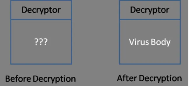
One of the simplest ways to hide virus signature is encryption.Virus body is en-crypted with different key so that no common signature is identified [23]. The simplest way to perform encryption is XORing virus body with a key. Virus has to decrypt itself before the execution and hence decryption routine exists in the virus. Cascade was the first DOS virus that implemented encryption [31]. Detection of such virus is possible without decrypting virus body. The decryptor routine remains common across all the generation of virus, so it is used as signature in virus definition [8]. Figure 1 shows before and after decryption status of encrypted virus.

Figure 1: Encrypted virus before and after decryption.

2.1.1.2 Polymorphic Virus

Polymorphic virus overcomes the drawback of constant decryption routine. It can create endless number of different decryption routines. Since the decryption routine along with the virus body varies from generation to generation, no common signature is identified [15]. Win95/Marburg and Win95/HPS were the first viruses that used 32-bit polymorphic engines [31]. Virus like Win32/Coke used multiple layer of encryption [31].

(16)

Code emulation can be used to detect polymorphic malware [22]. Virus code is executed in a virtual machine which leads to its decryption. Since all variants carry same virus body, once the virus is decrypted, it can be used as a signature for detection of other variants [20].

2.1.1.3 Metamorphic Virus

Metamorphic virus consists of an important part called mutation engine [18]. Instead of using encryption and decryption routine, entire body of a virus is changed using mutation engine while keeping the functionality intact. Mutation engine can be a part of a virus body or it can be separate from virus [33]. If mutation engine is a part of virus body, it needs to be morphed. This places restriction on the level of metamorphism that can be achieved. On the other hand, if mutation engine is separate from virus body, high degree of metamorphism can be achieved as muta-tion engine need not be morphed [34, 39]. We explained some of the metamorphic techniques in Chapter 3. Figure 2 shows different generations of the metamorphic virus.

2.1.2 Worms

Worms are self replicating malware. They are standalone [19]. Unlike viruses, worms intentionally spread themselves from one computer to other across the network. Viruses require human interaction (such as program execution) to spread, but worms don’t. Like viruses, worms rely on obfuscation techniques (such as metamorphism, polymorphism) to hide their presence.

Due to less human interaction, worms spread much faster as compared to viruses. For example, Melissa worm spreads very quickly as compared to other viruses [29].

(17)

Figure 2: Multiple shapes of a metamorphic virus body [14]

2.2 Detection Techniques

With the increase in number of malware, its detection technique has been evolved. Some detection techniques rely on static analysis while others depend on dynamic analysis. This section describes virus detection mechanisms used in an anti-virus software.

2.2.1 Signature Based Detection

Signature based detection is most commonly used malware detection technique. It involves searching for a known pattern (called as signature) in an executable. Antivirus software maintains large database consisting of unique signature for each virus [2]. When scanner scans an executable, it compares signature of the executable with the database and if any match is found, executable is considered to be infected. Signature based detection scheme is accurate, simple and fast [27]. The drawback

(18)

of this technique is that it requires up-to-date malware signature database. Also it cannot detect new virus because the signature of such virus is not present in the database. Simple obfuscation techniques like metamorphism, polymorphism can be used to evade signature based detection [20].

2.2.2 Anomaly Based Detection

In anomaly based detection, static and dynamic heuristics are used to detect malware. Static heuristic looks for suspicious structure like undocumented API calls, decryption loops [2, 38]. Dynamic heuristic such as code emulation analyzes suspicious activity of a program at runtime [38]. There are two phases in this technique -training and detection. In -training, scanner is trained to learn characteristics of normal and malicious program. In detection phase, it detects malicious program based on information gathered in the training phase [33]. Compared to signature based detection, anomaly based detection technique does a better job in detecting new virus. However, it has high number of false positives and false negatives [10].

2.2.3 Hidden Markov Model Based Detection

Hidden Markov Model (HMM) is a relatively new detection technique. Significant research has been done on Hidden Markov Model to detect metamorphic virus [1, 15, 40]. HMM is a probabilistic model and can be viewed as a machine learning technique. The notations used in HMM are shown in Table 3 [28]. A generic Hidden Markov Model is explained in Figure 3 whereXt andOtrepresents hidden state sequence and observation respectively. The Markov process is determined by the current state and the A matrix. We are able to observeOtwhich are related to the state of the Markov process by the matrix B.

(19)

Table 1: HMM Notations [28]

Symbol Description

T Length of the observed sequence N Number of states in the model

M Number of distinct observation symbols

O Observation sequence (O0,O1, . . . ,OT−1)

A State transition probability matrix

B Observation probability distribution matrix π Initial state distribution matrix

Figure 3: Generic Hidden Markov Model [28]

Research shows that HMMs are used in speech recognition [21] and software piracy detection [12]. There are two phases in HMM - training and detection. HMM is trained on input data and a training model is constructed. This training model is used to determine whether new observations are similar to the training model. Opcode sequence is extracted from same virus family and it is used to train HMM. Example of an extracted opcodes is shown in Figure 4. A long observation sequence is generated by concatenating opcode sequences from all virus files within same family [33]. Then this concatenated sequence is used to train HMM which is then used to detect and differentiate malware and benign files [15, 26, 40].

(20)

(21)

CHAPTER 3 Metamorphic Techniques

As mentioned in Chapter 2, the important part of metamorphic malware is a mutation engine. Mutation engine is capable of generating large number of differ-ent generations of virus whose functionality remains the same. Code obfuscation depends on program data and control flow [4, 41]. Data flow obfuscation consists of instruction substitution, dead code insertion, instruction permutation while control flow obfuscation consists of changing the control flow [4]. Virus writers employ differ-ent obfuscation techniques to avoid the detection of metamorphic virus. This chapter explains some of those techniques in detail.

3.1 Register Swap

Register swap is one of the simplest metamorphic technique. It changes regis-ter operand with an equivalent regisregis-ter without changing the opcode. Hence opcode sequence remains the same. The RegSwap metamorphic virus used register swap technique [6]. It used various registers in each generation without changing the func-tionality. Table 2 shows code fragment from some generation of W95/RegSwap virus.

3.2 Subroutine Permutation

Subroutine Permutation technique achieves code obfuscation by rearranging sub-routines from generation to generation. If there are n subroutines then there will be n! generations. Viruses like BadBoy, W32/Ghost implemented this technique [6]. BadBoy has 8 subroutines, so it can create 8! = 40320 generations. Figure 5 shows an example of BadBoy with 8 subroutines.

(22)

Table 2: Two generations of RegSwap [6]

a)

pop edx

mov edi, 0004h mov esi, ebp mov eax, 000Ch add edx, 0088h mov ebx, [edx]

mov [esi+eax*4+00001118], ebx

b)

pop eax

mov ebx, 0004h mov edx, ebp mov edi, 000Ch add eax, 0088h mov esi, [eax]

mov [edx+edi*4+00001118], esi

(23)

3.3 Dead Code Insertion

Dead code instructions may or may not get executed. In any case, it has no effect on the functionality of the program. Table 3 shows some kinds of dead code insertions.

Table 3: Example of dead code [31]

Instruction Description

add Reg,0 Add value 0 to register

mov Reg,Reg Transfer register value to itself

or Reg, 0 Logical OR operation of register with 0

NOP No operation

None of the below mentioned instructions in Table 3 change the value of the register. Dead code insertion is useful in evading malware detection which is based on statistical properties of the program. Dead code can create an unlimited number of virus copies. Dead code insertion technique is used in virus like Win95/Zperm [6] and metamorphic worm implemented in [26].

3.4 Instruction Substitution

In Instruction Substitution, an instruction or group of instructions is substi-tuted by another equivalent instruction or group of instructions. For example, the instruction xor eax, eaxwill be replaced by sub eax, eax. Both instructions zero contents of eax register but they use different opcodes. Instruction substitution is a powerful technique to evade signature based detection. However it is difficult to implement. Instruction substitution technique is used in W32/MetaPhor virus [6] and metamorphic worm implemented in [26].

(24)

3.5 Transposition

Transposition reorders instruction sequence without changing the overall func-tionality of the program. If two instructions are independent of each other then their order can be changed. For example :

1. mul Op1 Op2

2. mul Op3 Op4

Since these instructions are not dependent on each other, we can swap their order without affecting functionality of the code.

1. mul Op3 Op4

2. mul Op1 Op2

Similar technique is applied on group of instructions which are independent. This technique helps to evade signature based detection as order of execution is different.

3.6 Formal Grammar Mutation

Classic morphing engines can be considered as nondeterministic automata, since transitions are possible from every symbol to every other symbol [42]. A symbol is considered as a set of all possible instructions. In morphing engine, any instruction can be followed by any other instruction. By formalizing mutation techniques, we can apply formal grammar rules and create malicious copies with large amount of variation [33]. Figure 6 shows a simple polymorphic decryptor template and its two mutations using the formal grammar shown in Figure 7. With this decryptor template and formal grammar combination, it is possible to generate 960 decryptors [42].

(25)

Figure 6: A simple polymorphic decryptor and two variants [42]

Figure 7: Formal grammar for decryptor mutation [42]

3.7 Host Code Mutation

Some viruses mutate the code of host along with its own code in new genera-tion [13]. This is done by executing random code morphing routine. Win95/Bistro

(26)

virus uses host code emulation technique. The code morphing routine of Bistro uses morphing techniques like dead code insertion, instruction substitution, transposition etc. Win95/Bistro can be hard to repair, because the entry point of an application can be changed [32].

3.8 Code Integration

Win95/Zmist virus implemented code integration technique. Zmist virus decom-piles portable executable(PE) file to their smallest element, insert itself into code of PE file, regenerate code and data references and recompile the executable [31]. Due to this, Zmist integrate itself perfectly in an application and becomes hard to detect [31]

(27)

CHAPTER 4

Design and implementation

In this chapter we discuss the previous work on malware detection using function call graph analysis technique. Then we explain an algorithm to determine similarity between malware variants using the same technique.

4.1 Previous work

Traditional malware detection techniques depend on byte pattern or signature of the virus. The signature based detection ignores high level functionality of the virus. This technique can be easily defeated using obfuscation methods seen in Chapter 3. Function call graph technique relies on high level structure of the virus such as basic blocks and function calls [17]. Once call graph is created it can be treated as a malware signature and can be used to detect its variants.

The function call graph is created from the disassembled code of a malware ex-ecutable where vertices represent functions in the program and edges represent the caller-callee relationship between functions [17]. Then caller-callee relation, opera-tional code and graph coloring techniques are combined to measure similarity be-tween variants of known malware samples. A function call graph describes overall characteristics of a malware. Thus finding similarity between malware is equivalent to finding similarity between graphs. Ming et al. explained a technique to deter-mine a similarity between two malware variants using function call graph [17]. Their technique was tested on malicious software such as virus, backdoor, worms.

(28)

like NGVCK and MWOR. MWOR is a metamorphic worm generator that carries its own metamorphic engine. We used this technique to find similarity between malware variants as well as to differentiate malware and benign samples. Our testing results are explained in Chapter 5.

4.2 Overview of the function call graph

This section explain definition of function call graph and terminologies used in the paper. Then we explain function call graph construction technique.

4.2.1 Defining the function call graph

Function call graph G= (V, E) consists of vertices V and edges E where vertices represent functions and edges represent relationship between functions [17]. In an executable, functions are classified in two types as local functions and external func-tions. Local functions are written to perform specific task. External functions are system or library functions. In our experiment, local function starts withsub xxxxxx proc near and ends with sub xxxxxx endp where sub xxxxxx represents name of the function. Local functions carry different names in different programs even though their functionality is same. However, name of the external function is consistent in different programs.

4.2.2 Construction of function call graph

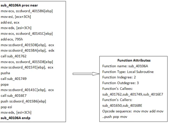
As a first step, a malware sample is disassembled using IDA Pro. Then we obtain the assembly code where all function names are labeled. Figure 8 shows snapshot of one function in NGVCK virus after its disassembly. It also shows attributes of the function added as vertex of the graph.

(29)

Figure 8: A function from NGVCK virus

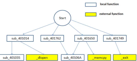
Then function call graph is built from assembly code. Figure 9 shows part of a function call graph for MWOR virus. As shown in Figure 9, the graph consists of local functions with the name pattern as sub xxxxxx and external function like

dlopen. Note that local function can call external functions but external functions cannot call local functions.

Breadth First Search (BFS) and Depth First Search (DFS) techniques are used in graph construction depending on the requirement. In the BFS technique, you start from first level nodes (root nodes) and continue scanning second level nodes and so on. In our technique we first go through all the entry point functions in a program and then traverse non - entry point functions called from each entry point functions. That means, entry point functions are at first level in the graph and non - entry point functions start from second level of the graph. Hence, in our technique Breadth

(30)

Figure 9: Part of the function call graph in MWOR virus

First Search approach is suitable for construction of the graph. The algorithm uses caller-callee relationship starting from the entry point function [24]. The algorithm starts with entry point functions and traverses each function’s instruction sequence to determine subroutine calls. Once all functions are processed, the function call graph is generated. Table 4 describes an algorithm used to generate the function call graph. First of all, algorithm traverses assembly code and determines function boundaries. All non - entry functions are stored in Functionset and all entry func-tions are stored inEntryFunctionSet. ThenFunctionQueueis initialized with entry functions. While queue is not empty, the algorithm dequeues from the front of the queue, stores the vertex in tailVertex and treats it as a caller. Then tailVertex

is inserted in the graph and its enqueFlagis set to true, to make sure that the same vertex is not enqueued again. Then the algorithm traverses instruction sequence of

tailVertex and determines its callee set.

Once the callee set is acquired, it is traversed one by one and stored in

headVertex. For each headVertex, it is checked whether the graph has an edge from tailVertex to headVertex. If there is an edge then caller’s out-degree and

(31)

callee’s in-degree is increased by one. Else, headVertex and its corresponding edge with tailVertex is inserted into graph. At the end, if enqueFlag of headVertex is not true, then it is set to true and headVertex is inserted at the end of the queue. The time complexity of this algorithm isO(|V| ∗ |E|) where V is the total number of vertices and E is the total number of edges [24].

4.3 Function Call Graph Similarity

Once function call graphs are constructed then similarity between two malware variants is determined by checking similarity between two graphs. The vertices of the graph are constructed from functions in the assembly code. Hence to find out similar-ity between two graphs we have to determine similar vertices in the graphs. Finding similar vertices in the graph is equivalent to finding similar function pairs in two mal-ware variants. The function matching based on string pattern is not useful because it can be easily defeated using different code obfuscation techniques. The external functions are easier to match as compared to local functions. The external functions are matched using their symbolic names. The local functions are not matched using symbolic names because two identical local functions from two different malware vari-ants have different names [17]. Also virus writer uses obfuscation techniques like dead code insertion, simple substitution to avoid detection. We propose a technique based on the opcode sequence and graph coloring mechanism to find similar local functions. This section explains algorithms used to match external and local functions.

4.3.1 Matching External Functions

External functions are provided by the operating system. They are also called as atomic functions. These functions make no further calls and have same names across

(32)

Table 4: Function call graph construction

// Input: Assembly file M, Output: Function call graph GM // Initializations

GM.V =φ and GM.E=φ

EntryFunctionSet =φ, FunctionSet = φ, FunctionQueue =φ, VertexSet =φ FunctionSet = ExtractFunction(M)

EntryFunctionSet = ExtractEntryFunction(M) FunctionQueue = InitQueue(EntryFunctionSet) while(FunctionQueue is not empty)

tailVertex = Dequeue(FunctionQueue) Insert tailVertex in GM

tailVertex.enqueFlag = true VertexSet = getCallee(tailVertex) for each vertex in VertexSet

if(vertex is not in FunctionSet) continue

endif

headVertex = vertex

// Construct an edge between tailVertex and headVertex if(e ∈GM.E) tailVertex.outdegree++ headVertex.indegree++ else Insert headVertex in GM Insert edge e inGM endif if(headVertex.enqueFlag == false)

Enqueue headVertex in FunctionQueue headVertex.enqueFlag = true endif next vertex end while return GM end

all executables [5]. In the graph theory, external functions are the leaf nodes with in-degree 1 and out-degree 0 [5]. External functions can be matched based on their symbolic names. For example, GetVersion function in one program can be matched

(33)

with same function in other program. Table 5 shows an algorithm used to match external functions [17].

Table 5: Algorithm to match external functions

// Input: Function call graph G1 and G2 Output: common vertex(G1, G2) ExternalfuncSet1 ←External function from G1

ExternalfuncSet2 ←External function from G2 Copy vertices from G1 intoUs

Copy vertices from G2 intoVs

foreach vertex Usi ExternalfuncSet1 do foreach vertex Vsj ExternalfuncSet2 do

if(Usi.name = Vsj.name)

common vertex(G1, G2)← common vertex(G1, G2)∪ (Usi,Vsj) Remove Usi fromUs

Remove Vsj fromVs end

end end

External functions are extracted from graph G1, G2 and copied into

ExternalfuncSet1 and ExternalfuncSet2 respectively. Then both sets are tra-versed to find out same symbolic names. If there is match in name, then that vertex is copied into common vertex pair.

4.3.2 Finding similar local functions based on same external functions

Two local functions are considered to be matching if they call two or more similar external functions [5]. Table 6 shows an algorithm used to find matching function pair [17].

All local functions in graph G1, G2 are traversed and checked if they call same external functions. If the count of these common external functions is greater than or equal to 2, then those local functions are copied into common vertex pair.

(34)

Table 6: Algorithm to match local functions based on external functions

// Input: Function call graph G1 and G2,Us,Vs,common vertex(G1, G2) //Output: common vertex(G1, G2)

foreach vertex Usi Us do foreach vertex Vsj Vs do

if(ExternalFunction(Usi)∩ ExternalFunction(Vsj) ≥ 2) then common vertex(G1, G2) ←common vertex(G1, G2) ∪ (Usi,Vsj) Remove Usi from Us

end end

4.3.3 Matching local functions based on opcode sequence

Each vertex in the call graph is colored depending on the instructions used in this function. Then cosine similarity method along with color similarity is used to find similar functions. All x86 instructions are classified in 15 classes according to their function as shown in Table 7.

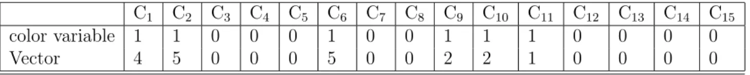
A 15 bit color variable is used to color a vertex in the graph. This variable is initialized to 0. When an instruction from a particular class appears in the function, corresponding bit of color variable is set to 1. We have also created a vector which holds number of corresponding class instructions appearing in a local function. Ta-ble 8 contains function from MWOR virus and TaTa-ble 9 shows corresponding class variable and vector.

(35)

Table 7: x86 instruction classification [17]

Class Data Description

C1 Data data transfer such as mov

C2 Stack Stack Operation

C3 Port In and out

C4 Lea Destination address trans-mit

C5 Flag Flag transmit

C6 Arithmetic shift, rotate etc.

C7 Logic bitbyte operation

C8 String String operation

C9 Jump Unconditional transfer

C10 Branch Conditional transfer

C11 Loop Loop control

C12 Halt Stop instruction execution

C13 Bit Bit test and bit scan

C14 Processor Processor control

C15 Float Floating point operation

We created two vectors X = (x1, x2, ..., x15) and Y = (y1, y2, ..., y15) from two function pairs. Then cosine similarity between these two vectors is calculated as shown in formula (1) [17]: sim(X, Y) = P15 i=1xi.yi q P15 i=1x2i. q P15 i=1yi2 (1)

When cosine similarity is greater than or equal to certain threshold value α and two color variables are same then two function pairs from two different executables are considered to be color similar function pairs. Table 10 describes an algorithm used to find the color similarity between two function pairs [17].

The algorithm takes functions f1 and f2 as input and calculates the cosine sim-ilarity. First, it generates two color variables color1 and color2 from f1 and f2. If

(36)

Table 8: The function from MWOR virus

sub 40448C proc near push rbp

mov rbp, rsp push rbx sub rsp, 8

mov rax, cs:CTOR LIST

cmp rax, 0FFFFFFFFFFFFFFFFh jz short loc 4051AF

mov ebx, offset CTOR LIST sub rbx, 8

call CTOR LIST mov rax, [rbx]

cmp rax, 0FFFFFFFFFFFFFFFFh jnz short loc 4051A0

add rsp, 8 pop rbx pop rbp call sub 40238C pop esi retn sub 40448C endp

Table 9: The color variable and the vector of MWOR virus

C1 C2 C3 C4 C5 C6 C7 C8 C9 C10 C11 C12 C13 C14 C15 color variable 1 1 0 0 0 1 0 0 1 1 1 0 0 0 0

Vector 4 5 0 0 0 5 0 0 2 2 1 0 0 0 0

these two variables are similar then two vectors are generated from f1 and f2. Then cosine similarity between vector1 and vector2 is calculated using the formula de-scribed above. In order to get more accurate results, two extra constraints are added as length of the function (number of bytes of instruction in the function) and degree of the function (total of in-degrees and out-degrees in function). The in-degree of

(37)

Table 10: Algorithm to find color similarity between two functions

// Input: Functions f1 and f2

//Output: color similarity betweenf1 and f2 color1← getColorSequence from f1

color2← getColorSequence from f2 if(color1=color2)

vector1← getVector fromf1 vector2← getVector fromf2

color sim← calculate cosine similarity between vector1 and vector2 end

return color sim

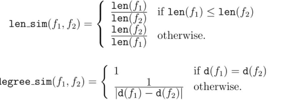
a function A is total number of functions calling A. The out-degree of function A is total number of functions called from A. Therefore, two functions are said to be similar if, cosine similarity is greater than or equal to α, length similarity(len sim) is greater than or equal to β and degree similarity(degree sim) is greater than or equal to γ where len sim and degree sim are calculated using equation (2) and (3) respectively. len sim(f1, f2) =      len(f1) len(f2) if len(f1)≤len(f2) len(f2) len(f1) otherwise. (2) degree sim(f1, f2) = ( 1 if d(f1) =d(f2) 1 |d(f1)−d(f2)| otherwise. (3) where len(f1) is number of bytes of instructions in the function f1, len(f2) is number of bytes of instructions in the function f2, d(f1) is degree of function f1 and

d(f2) is degree of function f2. Value of α, β and γ were taken as 0.98, 0.83 and 0.5 respectively based on experiments. Table 11 describes an algorithm used to find matching function pair based on color similarity [17].

(38)

Table 11: Algorithm to match local functions based on color similarity

foreach vertex Usi Us do foreach vertex Vsj Vs do

if(color sim(Usi,Vsj)≥ α ∩ len sim(Usi,Vsj) ≥β ∩

degree sim(Usi,Vsj) ≥ γ) then

common vertex(G1, G2) ←common vertex(G1, G2) ∪ (Usi,Vsj) Remove Usi from Us

end end

4.3.4 Matching local functions based on matched neighbors

When two vertices match then, it is more likely that their neighbors will match too [17]. In a graph, neighbors of vertex are its successors and predecessors. As shown in Figure 10 vertex A of one graph is matched with vertex B of other. Then chances are that vertices U,V and W from one graph can match with vertices X,Y and Z from other graph because they are direct neighbors to previously matched vertices. In Figure 10 vertices of same color are treated as similar.

(39)

Table 12 describes algorithm is used to find matching function pairs based on matched successor [17].

Table 12: Algorithm to match local functions based on matched successor

vertexQueue ← InitvertexQueue(common vertex(G1, G2)) while (vertexQueue is not empty)

(u,v)← vertexQueue.dequeue()

foreach vertex Usi successor(u) ∩ Us do foreach vertex Vsj successor(v) ∩ Vs do

if(color relaxed sim(Usi,Vsj) ≥ δ) then

common vertex(G1, G2) ← common vertex(G1, G2)∪ (Usi,Vsj) Remove Usi fromUs Remove Vsj from Vs vertexQueue.enqueue(Usi,Vsj) end end end end

return common vertex(G1, G2)

A queue is initialized with the common vertex. Then the algorithm runs until the queue becomes empty. The head of the queue is removed. As shown in line 6,7 successor vertices are traversed one by one from common vertex pair. If their color relaxed similarity score is greater than or equal to δ then successor vertices pair is considered to be similar. Finding color relaxed similarity score is same as finding color similarity between two function pairs except the constraint of similar color variable is removed. Here δ is equal to 0.97 based on experiments. The algorithm for finding matched predecessor is similar to above except for the fact that instead of successors, predecessors are traversed from common vertex pair.

(40)

4.3.5 Similarity between function call graph

Once we have found common vertex pairs from two call graphs, common edges between graphs are calculated. When vertices A, B from one graph are similar to vertices C, D from other graph respectively and there is an edge between A,B in first graph and between C,D in other then that edge is said to be common in two graphs. Similarity between two function call graph is calculated as shown in Formula (4) [17]:

sim(G1, G2) =

2|common edge(G1, G2)|

|E(G1)|+|E(G2)|

∗100 (4) where |common edge(G1, G2)| represents common edges between call graph G1 and

G2. |E(G1)|+|E(G2)| represents total number of edges in graph G1 and G2. If similarity score is closer to 1, then there is more similarity between two virus files.

(41)

CHAPTER 5 Experiments

We used Java to implement the algorithm mentioned in Chapter 4. The Next Generation Virus Generation kit (NGVCK) and Metamorphic Worm (MWOR) are used to test our implementation. Cygwin and Linux library files are used as benign files during the testing. The metamorphic worm has been developed to defeat Hidden Markov Model (HMM) detection technique [26]. It uses two morphing techniques:

• Dead code insertion

• Instruction substitution

The metamorphic generator produces copies of the same virus which are different across all generations. Since the dead code is inserted directly from benign files, they look similar. The metamorphic generator uses padding ratios to generate viruses. The padding ratio is a number of dead code instructions to number of instructions in virus which constitute its functionality [25].

5.1 Test Data

Our test data consists of 50 NGVCK virus files, total 140 MWOR virus files with padding ratios of 0.5, 1.0, 1.5, 2.0, 2.5, 3.0 and 4.0. In benign files we used 50 Cygwin and 20 Linux library files.

(42)

5.2 Test Results

The algorithm takes two files as input and calculates similarity between them. Firstly, we calculate similarity score between two virus files. If the similarity score is closer to 1, the two copies are similar. Secondly, we calculate similarity score between virus and benign file. Thus, we are not only able to find out similar copies of virus but also differentiate between virus and benign files. We used scatter graph and Area under ROC curve (AUC) to evaluate performance of the detection system. AUC of 1 represents a perfect system and an AUC of 0.5 or less represents worst system. This section describes test results obtained from the experiments.

5.2.1 NGVCK Testing Results

We tested our detection system on NGVCK virus. Results show that our detec-tion system is not only able to find similar copies of NGVCK virus but also differen-tiate between virus and benign files.

Figure 11 shows similarity scores obtained by detection system on NGVCK viruses. It shows 0.95 as maximum and 0.46 as minimum score for metamorphic virus files. Figure 12 shows area under curve (AUC) statistics for NGVCK virus family.

5.2.2 MWOR Testing Results

We tested our detection system on MWOR with different padding ratios. Results show that, when padding ratio is greater than or equal to 2.5 there is misclassification between virus and benign files. Figures 13 to 19 show similarity scores obtained by detection system for various padding ratios in MWOR virus.

(43)

Figure 11: Similarity score NGVCK virus family

Figure 13 is a scatter graph and it shows 0.87 as maximum and 0.56 as minimum score of metamorphic virus files for padding ratio 0.5. In Figure 13 we can clearly see a separation between virus vs. virus scores and virus vs benign scores.

As more and more dead code is inserted into virus file from benign files, similarity scores between virus files start reducing. Figure 15 shows 0.47 as minimum score of metamorphic virus files for padding ratio 1.5. As per the results, we are able to separate virus vs. virus score from virus vs. benign score.

Figure 16 shows that the minimum score of metamorphic virus files is 0.44 for padding ratio 2.0. As per the results, we are still able to separate virus vs. virus

(44)

Figure 12: ROC Curve for NGVCK virus family

score from virus vs. benign score.

Figure 17 shows that there is misclassification between virus and benign files for padding ratio 2.5. As shown in Table 13 the area under curve for 2.5 padding ratio is 0.9999 , which confirms the misclassification.

Figure 18 also shows that there is a higher degree of misclassification between virus and benign files for padding ratio 3.0 as compared to 2.5. As shown in Table 13 the area under curve for 3.0 padding ratio is 0.9989, which confirms the misclassifi-cation.

Figure 19 also shows that there is a higher degree of misclassification between virus and benign files for padding ratio 4.0 as compared to 3.0. As shown in Table 13 the area under curve for 4.0 padding ratio is 0.9979, which confirms the

(45)

misclassifi-Figure 13: Similarity scores of MWOR with padding ratio of 0.5

cation.

Figure 20 and 21 show area under ROC curves (AUC) for MWOR virus with different padding ratios. Table 13 represents ROC AUC statistics for different padding ratios.

(46)

Figure 14: Similarity scores of MWOR with padding ratio of 1.0

Table 13: ROC AUC statistics for different padding ratios of MWOR

Padding-ratio AUC 0.5 1 1.0 1 1.5 1 2.0 1 2.5 0.9999 3.0 0.9989 4.0 0.9979

(47)

(48)

(49)

(50)

(51)

(52)

(53)

(54)

5.2.3 Comparison with other detection systems

5.2.3.1 Comparison with opcode based graph detection system

We compared our detection technique with the opcode based graph detection technique mentioned in [23]. As mentioned in [26], opcode based graph similarity technique misclassified benign files and MWOR virus with padding ratio greater than or equal to 1.5. In our proposed technique, this misclassification starts from padding ratio greater than or equal to 2.5.

5.2.3.2 Comparison with HMM Detection Technique

Hidden Markov Model detection technique was tested on MWOR virus with different padding ratio [26]. After comparing our results with the result obtained from HMM, our technique performs better. ROC statistics for both techniques is shown in Table 14.

Table 14: ROC AUC statistics of function call graph and HMM technique

Padding-ratio AUC call graph AUC HMM AUC simple substitution

0.5 1 1 1 1.0 1 0.99 1 1.5 1 0.9625 0.9980 2.0 1 0.9725 0.9985 2.5 0.9999 0.8325 0.9859 3.0 0.9989 0.8575 0.9725 4.0 0.9979 0.8225 0.9565

Figure 22 is a line graph showing comparison of area under curve statistics for HMM and function call graph based malware detection techniques.

(55)

(56)

CHAPTER 6

Conclusion and future work

We designed and implemented function call graph technique for the metamorphic malware detection. This technique makes use of cosine similarity based on opcodes and graph coloring technique to identify similarity between two malware variants. This technique finds out similar function pairs from two executables. The func-tion matching is based on four parts - matching external funcfunc-tions with same name, matching local functions based on identical external functions, matching local func-tions based on opcode sequence and matching local funcfunc-tions based on their matched neighbors. Then at the end similarity between two call graphs is calculated based on common edges. This is also helpful in differentiating malware from benign files. We tested our implementation on NGVCK and MWOR family viruses.

Results show that we can easily set threshold for NGVCK family that clearly separates NGVCK viruses and the benign files. Our detection technique achieves 100% accuracy when tested on MWOR family virus with padding ratio 2.0 and below. The misclassification starts from the padding ratio 2.5 onwards as shown in figure 13. We also found that our detection technique performs better than other graph based and HMM based detection techniques mentioned in [23] and [26] respectively.

Currently the function call graph detection technique detects NGVCK and MWOR metamorphic viruses. Going forward, it would be beneficial to consider more recent malware. The results clearly indicates that in case of MWOR family virus, misclassification between malware and benign file starts when a block of code from benign files is used for morphing. Therefore, some modifications are necessary to

(57)

deal with this limitation. In this paper, we concentrated on the metamorphic viruses as they are harder to detect. We can extend this detection technique on the other types of malware like rootkit, backdoor. Also it might be useful to create the hybrid model based on proposed technique and opcode graph similarity technique to gener-ate stronger metamorphic virus detector.. In the future this detection technique can be tested on metamorphic generator designed from LLVM IR byte code [33].

(58)

LIST OF REFERENCES

[1] S. Attaluri, S. McGhee and M. Stamp, Profile hidden markov models and meta-morphic virus detection, Journal in Computer Virology, 5(2):151–169, 2009 [2] J. Aycock, Computer Viruses and Malware, Advances in Information Security,

Springer-Verlag, New York, 2006

[3] D. Bilar, On callgraphs and generative mechanisms,Journal in Computer Virol-ogy, 3(4):285–297, 2007

[4] J. Borello, Code obfuscation techniques for metamorphic viruses, Journal in Computer Virology, 4(3):211–220, 2008

[5] E. Carrera and G. Erdelyi, Digital genome mapping-advanced binary malware analysis, In: Proceeding Virus Bulletin Conference, 187–197, 2004

[6] Computer Virus Creation Kit,

http://www.informit.com/articles/article.aspx?p=366890&seqNum=6

[7] M. Christodorescu, S. Jha and C. Kruegel, Mining specifications of malicious behavior, Proceedings of the 6th joint meeting of the European Software Engi-neering Conference and the ACM SIGSOFT Symposium on the Foundations of Software Engineering, 5–14, 2007

[8] E. Filiol, Computer Viruses: From Theory to Applications, Volume 1, Birkhauser, pp.19–38, 2005

[9] Hex-Rays, S.A.:IDA Pro 5.5

http://www.hex-rays.com/products/ida/index.shtml

[10] N. Idika and A. Mathur, A Survey of Malware Detection Techniques, Technical report, Department of Computer Science, Purdue University, 1969

http://www.serc.net/systems/files/SERC-TR-286.pdf

[11] A. Karnik, S. Goswami and R. Guha, Detecting obfuscated viruses using cosine similarity analysis, Proceedings of the First Asia International Conference on Modelling Simulation, 165–170, 2007

[12] S. Kazi and M. Stamp, Hidden Markov Models for Software Piracy Detection, Information Security Journal: A Global perspective, 22(3):140–149, 2013

(59)

[13] E. Konstantinou and S. Wolthusen, Metamorphic Virus: Analysis and Detection, Technical Report

http://www.ma.rhul.ac.uk/static/techrep/2008/RHUL-MA-2008-02.pdf

[14] A. Lakhotia, Are Metamorphic Viruses Really Invincible?, Virus Bulletin, De-cember 2004

http://www.iscas2007.org/~arun/papers/invincible-complete.pdf

[15] D. Lin and M. Stamp, Hunting for undetectable metamorphic viruses, Journal in Computer Virology, 7(3):201–214, August 2011

[16] M. Masrom and B. Rad, Metamorphic Virus Variants Classification using Op-code Frequency Histogram,

http://arxiv.org/ftp/arxiv/papers/1104/1104.3228.pdf

[17] X. Ming, W. Lingfei, Q. Shuhui, X. Jian, Z. Haiping, R. Yizhi and Z. Ning, A similarity metric method of obfuscated malware using function-call graph, Journal in Computer Virology and Hacking Techniques, 9(1):35–47, 2013

[18] C. Nachenberg, Computer virus-antivirus coevolution, Communications of the ACM, 40(1):46–51, 1997

[19] Panda Security, Virus, worms, trojans and backdoors: Other harmful relatives of viruses, 2011,

http://www.pandasecurity.com/homeusers-cms3/security-info/about-malware/

generalconcepts/concept-2.html

[20] S. Priyadarshi, Metamorphic Detection via Emulation, Master’s Projects, Paper 177

http://scholarworks.sjsu.edu/etd_projects/177

[21] L.R.Rabiner, A tutorial on hidden Markov Model and selected applications in speech recognition, Proceeding of the IEEE, 77(2):257–286, February 1989 [22] B. Rad, M. Masrom and S. Ibrahim, Evolution of Computer Virus Concealment

and Anti-Virus Techniques: A Short Survey, IJCSI International Journal of Computer Science Issues, 8(1):113–121, 2011

[23] N. Runwal, R. Low and M. Stamp, Opcode Graph Similarity and Metamorphic Detection, Journal in Computer Virology, 8(1-2):37–52, May 2012

[24] S. Shang,N. Zhen, J. Xu, M. Xu and H. Zhang, Detecting malware variants via function-call graph similarity, 5th International Conference Malicious and Unwanted Software, 113–120, 2010

(60)

[25] G. Shanmugam, R. Low and M. Stamp, Simple substitution distance and metamorphic detection, Journal in Computer Virology and Hacking Techniques, 9(3):159–170, August 2013

[26] S. Sridhara and M. Stamp, Metamorphic worm that carries its own morphing engine,Journal in Computer Virology and Hacking Techniques, 9(2):49–58, 2012 [27] M. Stamp,Information Security: Principles and Practice, second edition, Wiley,

2011

[28] M. Stamp, A revealing introduction to hidden markov model, 2012 http://www.cs.sjsu.edu/~stamp/RUA/HMM.pdf

[29] Symantec, Learn More About Viruses and Worms, Symantec Antivirus Research Center,

http://www.symantec.com/avcenter/reference/worm.vs.virus.pdf

[30] Symantec, Internet Security Threat Report, Volume 17, Technical report, Symantec Corporation

http://www.symantec.com/content/en/us/enterprise/other_resources /b-istr_main_report_2011_21239364.en-us.pdf

[31] P. Szor and P. Ferrie, Hunting For Metamorphic, In Virus Bulletin Conference, September 2001

[32] P. Szor, The new 32-bit medusa Virus Bulletin 8–10, December 2000

[33] T. Tamboli, T. Austin and M. Stamp, Metamorphic Code Generation from LLVM IR Bytecode, to appear in Journal in Computer Virology and Hacking Techniques

[34] The Mental Driller, Metamorphism in practice or “How I made MetaPHOR and what I’ve learnt”, 2002

http://vx.netlux.org/lib/vmd01.html [35] Virus Construction Kit

http://computervirus.uw.hu/ch07lev1sec7.html [36] Virus Creation Tools, VX Heavens

http://oktridarmadi.blogspot.com/2009/09/virus-creation-tools-vx-heavens.html [37] VX Heavens

http://download.adamas.ai/dlbase/Stuff/VX%20Heavens %20Library/static/vdat/creatrs1.htm

[38] G. Wagener, R. State and A. Dulaunoy, Malware behaviour analysis, Journal in Computer Virology, 4(4): 279–287, 2008

(61)

[39] A. Walenstein, R. Mathur, M. Chouchane and A. Lakhotia, The design space of metamorphic malware,In Proceedings of the 2nd International Conference on Information Warfare, 2007

[40] W. Wong and M. Stamp, Hunting for metamorphic engines,Journal in Computer Virology, 2(3):211–219, 2006

[41] I. You and K. Yim, Malware obfuscation techniques: a brief survey, Interna-tional Conference on Broadband, Wireless Computing, Communication and Ap-plications, 297-300, 2010

[42] P. Zbitskiy, Code mutation techniques by means of formal grammars and au-tomatons. Journal in Computer Virology, 5(3):199-207, August 2009

(62)

APPENDIX

Additional Experiments

A.1 Experiment 1

Function call graph detection technique is based on analyzing functions. If we insert dead code from benign files into MWOR files, it should degrade the score. We inserted up to 5 dead code functions and for each function made up to 5 calls. In these 25 cases we calculated area under the curve as shown in Table A.15.

A.2 Experiment 2

We performed in-line and out-line of functions in MWOR files. In-lining is done by replacing function call with actual function. Out-lining is done by taking a section of code and writing it into the function. In-line and out-line makes the function call graph of MWOR different from each other. We did an experiment on MWOR with dead code ratio 2.0. We did up to 5 function in-lining and for each in-line made up to 5 function out-line. In these 25 cases we calculated area under the curve as shown in Table A.16.

(63)

Table A.15: AUC values of function calls Number of Functions 1 2 3 4 5 1 call/function 0.999907 0.999253 0.993304 0.989721 0.991989 2 call/function 0.999907 0.992879 0.992678 0.993026 0.993506 3 call/function 0.999659 0.993962 0.992763 0.99243 0.994481 4 call/function 0.999458 0.993931 0.989806 0.992082 0.993653 5 call/function 0.999551 0.993544 0.990023 0.991586 0.993204

Table A.16: AUC values of function in-line and out-line

Number of in-line functions 1 2 3 4 5

1 outline/in-line function 0.994 0.986888 0.982111 0.961444 0.954111 2 outline/in-line function 0.988222 0.982555 0.981777 0.973555 0.960444 3 outline/in-line function 0.972222 0.972888 0.965888 0.964333 0.96 4 outline/in-line function 0.967823 0.965788 0.976045 0.962912 0.973555 5 outline/in-line function 0.964545 0.962698 0.97239 0.965861 0.977333