Joint Emotion Analysis via Multi-task Gaussian Processes
Daniel Beck† Trevor Cohn‡ Lucia Specia†
†Department of Computer Science, University of Sheffield, United Kingdom {debeck1,l.specia}@sheffield.ac.uk
‡Computing and Information Systems, University of Melbourne, Australia [email protected]
Abstract
We propose a model for jointly predicting multiple emotions in natural language sen-tences. Our model is based on a low-rank coregionalisation approach, which com-bines a vector-valued Gaussian Process with a rich parameterisation scheme. We show that our approach is able to learn correlations and anti-correlations between emotions on a news headlines dataset. The proposed model outperforms both single-task baselines and other multi-single-task ap-proaches.
1 Introduction
Multi-task learning (Caruana, 1997) has been widely used in Natural Language Processing. Most of these learning methods are aimed for Do-main Adaptation (Daum´e III, 2007; Finkel and Manning, 2009), where we hypothesize that we can learn from multiple domains by assuming sim-ilarities between them. A more recent use of multi-task learning is to model annotator bias and noise for datasets labelled by multiple annotators (Cohn and Specia, 2013).
The settings mentioned above have one aspect in common: they assume some degree of posi-tive correlation between tasks. In Domain Adap-tation, we assume that some “general”, domain-independent knowledge exists in the data. For an-notator noise modelling, we assume that a “ground truth” exists and that annotations are some noisy deviations from this truth. However, for some set-tings these assumptions do not necessarily hold and often tasks can be anti-correlated. For these cases, we need to employ multi-task methods that are able to learn these relations from data and correctly employ them when making predictions, avoiding negative knowledge transfer.
An example of a problem that shows this be-haviour is Emotion Analysis, where the goal is to
automatically detect emotions in a text (rava and Mihalcea, 2008; Mihalcea and Strappa-rava, 2012). This problem is closely related to Opinion Mining (Pang and Lee, 2008), with sim-ilar applications, but it is usually done at a more fine-grained level and involves the prediction of a set of labels (one for each emotion) instead of a single label. While we expect some emotions to have some degree of correlation, this is usually not the case for all possible emotions. For instance, we expectsadnessandjoyto be anti-correlated.
We propose a multi-task setting for Emotion Analysis based on a vector-valued Gaussian Pro-cess (GP) approach known as coregionalisation
( ´Alvarez et al., 2012). The idea is to combine a GP with a low-rank matrix which encodes task corre-lations. Our motivation to employ this model is three-fold:
• Datasets for this task are scarce and small so we hypothesize that a multi-task approach will results in better models by allowing a task to borrow statistical strength from other tasks;
• The annotation scheme is subjective and very fine-grained, and is therefore heavily prone to bias and noise, both which can be modelled easily using GPs;
• Finally, we also have the goal to learn a model that shows sound and interpretable correlations between emotions.
2 Multi-task Gaussian Process Regression
Gaussian Processes (GPs) (Rasmussen and Williams, 2006) are a Bayesian kernelised framework considered the state-of-the-art for regression. They have been recently used success-fully for translation quality prediction (Cohn and Specia, 2013; Beck et al., 2013; Shah et al., 2013)
and modelling text periodicities (Preotiuc-Pietro and Cohn, 2013). In the following we give a brief description on how GPs are applied in a regression setting.
Given an input x, the GP regression assumes that its output y is a noise corrupted version of a latent function evaluation, y = f(x) +η, where
η ∼ N(0, σ2
n) is the added white noise and the functionfis drawn from a GP prior:
f(x)∼ GP(µ(x), k(x,x0)), (1)
whereµ(x)is themeanfunction, which is usually the 0 constant, and k(x,x0) is the kernel or co-variancefunction, which describes the covariance between values off at locationsxandx0.
To predict the value for an unseen inputx∗, we
compute the Bayesian posterior, which can be cal-culated analytically, resulting in a Gaussian distri-bution over the outputy∗:1
y∗ ∼ N(k∗(K+σnI)−1yT, (2)
k(x∗,x∗)−kT∗(K+σnI)−1k∗),
where K is the Gram matrix
corre-sponding to the covariance kernel evalu-ated at every pair of training inputs and k∗ = [hx1,x∗i,hx2,x∗i, . . . ,hxn,x∗i] is the
vector of kernel evaluations between the test input and each training input.
2.1 The Intrinsic Coregionalisation Model By extending the GP regression framework to vector-valued outputs we obtain the so-called coregionalisation models. Specifically, we employ a separable vector-valued kernel known as Intrin-sic Coregionalisation Model(ICM) ( ´Alvarez et al., 2012). Considering a set ofDtasks, we define the corresponding vector-valued kernel as:
k((x, d),(x0, d0)) =kdata(x,x0)×Bd,d0, (3)
where kdata is a kernel on the input points (here a Radial Basis Function, RBF),dandd0 are task
or metadata information for each input and B ∈ RD×D is the coregionalisation matrix, which en-codes task covariances and is symmetric and posi-tive semi-definite.
A key advantage of GP-based modelling is its ability to learn hyperparameters directly from data
1We refer the reader to Rasmussen and Williams (2006,
Chap. 2) for an in-depth explanation of GP regression.
by maximising the marginal likelihood:
p(y|X,θ) =
Z
fp(y|X,θ, f)p(f). (4) This process is usually performed to learn the noise variance and kernel hyperparameters, in-cluding the coregionalisation matrix. In order to do this, we need to consider how B is parame-terised.
Cohn and Specia (2013) treat the diagonal val-ues of B as hyperparameters, and as a conse-quence are able to leverage the inter-task trans-fer between each independent task and the global “pooled” task. They however fix non-diagonal val-ues to 1, which in practice is equivalent to assum-ing equal correlation across tasks. This can be lim-iting, in that this formulation cannot model anti-correlations between tasks.
In this work we lift this restriction by adopting a different parameterisation ofB that allows the learning of all task correlations. A straightforward way to do that would be to consider every corre-lation as an hyperparameter, but this can result in a matrix which is not positive semi-definite (and therefore, not a valid covariance matrix). To en-sure this property, we follow the method proposed by Bonilla et al. (2008), which decomposesB us-ing Probabilistic Principal Component Analysis:
B=UΛUT +diag(α), (5) where U is an D×R matrix containing the R
principal eigenvectors and Λ is a R ×R diago-nal matrix containing the corresponding eigenval-ues. The choice ofRdefines therankofUΛUT, which can be understood as the capacity of the manifold with which we model theDtasks. The vectorα allows for each task to behave more or less independently with respect to the global task. The final rank of B depends on both terms in Equation 5.
For numerical stability, we use the incomplete-Cholesky decomposition over the matrixUΛUT, resulting in the following parameterisation forB:
to additional non-convexities in the log likelihood objective. In our experiments we evaluate this be-haviour empirically by testing a range of ranks for each setting.
The low-rank model can subsume the ones pro-posed by Cohn and Specia (2013) by fixing and tying some of the hyperparameters:
Independent: fixing˜L=0andα=1; Pooled: fixing˜L=1andα=0;
Combined: fixing ˜L = 1 and tying all compo-nents ofα;
Combined+: fixing˜L=1.
These formulations allow us to easily replicate their modelling approach, which we evaluate as competitive baselines in our experiments.
3 Experimental Setup
To address the feasibility of our approach, we pro-pose a set of experiments with three goals in mind:
• To find our whether the ICM is able to learn sensible emotion correlations;
• To check if these correlations are able to im-prove predictions for unseen texts;
• To investigate the behaviour of the ICM model as we increase the training set size. Dataset We use the dataset provided by the “Af-fective Text” shared task in SemEval-2007 (Strap-parava and Mihalcea, 2007), which is composed of1000news headlines annotated in terms of six emotions: Anger, Disgust, Fear, Joy, Sadnessand
Surprise. For each emotion, a score between0and
100is given,0meaning total lack of emotion and
100maximum emotional load. We use 100 sen-tences for training and the remaining900for test-ing.
Model For all experiments, we use a Radial Ba-sis Function (RBF) data kernel over a bag-of-words feature representation. Words were down-cased and lemmatized using the WordNet lemma-tizer in the NLTK2toolkit (Bird et al., 2009). We then use the GPy toolkit3 to combine this kernel with a coregionalisation model over the six emo-tions, comparing a number of low-rank approxi-mations.
2http://www.nltk.org
3http://github.com/SheffieldML/GPy
Baselines and Evaluation We compare predic-tion results with a set of single-task baselines: a Support Vector Machine (SVM) using an RBF kernel with hyperparameters optimised via cross-validation and a single-task GP, optimised via like-lihood maximisation. The SVM models were trained using the Scikit-learn toolkit4 (Pedregosa et al., 2011). We also compare our results against the ones obtained by employing the “Combined” and “Combined+” models proposed by Cohn and Specia (2013). Following previous work in this area, we use Pearson’s correlation coefficient as evaluation metric.
4 Results and Discussion
4.1 Learned Task Correlations
Figure 1 shows the learned coregionalisation ma-trix setting the initial rank as 1, reordering the emotions to emphasize the learned structure. We can see that the matrix follows a block structure, clustering some of the emotions. This picture shows two interesting behaviours:
• Sadnessandfearare highly correlated.Anger
and disgust also correlate with them, al-though to a lesser extent, and could be con-sidered as belonging to the same cluster. We can also see correlation betweensurpriseand
joy. These are intuitively sound clusters based on the polarity of these emotions.
• In addition to correlations, the model learns anti-correlations, especially between
joy/surpriseand the other emotions. We also note thatjoyhas the highest diagonal value, meaning that it gives preference to indepen-dent modelling (instead of pooling over the remaining tasks).
Inspecting the eigenvalues of the learned ma-trix allows us to empirically determine its result-ing rank. In this case we find that the model has learned a matrix of rank 3, which indicates that our initial assumption of a rank 1 coregionalisa-tion matrix may be too small in terms of modelling capacity5. This suggests that a higher rank is justified, although care must be taken due to the local optima and overfitting issues cited in§2.1.
4http://scikit-learn.org
5The eigenvalues were592,62,86,4,3×10−3and9×
Anger Disgust Fear Joy Sadness Surprise All
SVM 0.3084 0.2135 0.3525 0.0905 0.3330 0.1148 0.2603
Single GP 0.1683 0.0035 0.3462 0.2035 0.3011 0.1599 0.3659
ICM GP (Combined) 0.2301 0.1230 0.2913 0.2202 0.2303 0.1744 0.3295
ICM GP (Combined+) 0.1539 0.1240 0.3438 0.2466 0.2850 0.2027 0.3723
ICM GP (Rank 1) 0.2133 0.1075 0.3623 0.2810 0.3137 0.2415 0.3988
[image:4.595.89.512.63.158.2]ICM GP (Rank 5) 0.2542 0.1799 0.3727 0.2711 0.3157 0.2446 0.3957
[image:4.595.77.280.241.399.2]Table 1: Prediction results in terms of Pearson’s correlation coefficient (higher is better). Boldface values show the best performing model for each emotion. The scores for the “All” column were calculated over the predictions for all emotions concatenated (instead of just averaging over the scores for each emotion).
Figure 1: Heatmap showing a learned coregional-isation matrix over the emotions.
4.2 Prediction Results
Table 1 shows the Pearson’s scores obtained in our experiments. The low-rank models outper-formed the baselines for the full task (predicting all emotions) and for fear, joy and surprise sub-tasks. The rank 5 models were also able to out-perform all GP baselines for the remaining emo-tions, but could not beat the SVM baseline. As expected, the “Combined” and “Combined+” per-formed worse than the low-rank models, probably due to their inability to model anti-correlations.
4.3 Error analysis
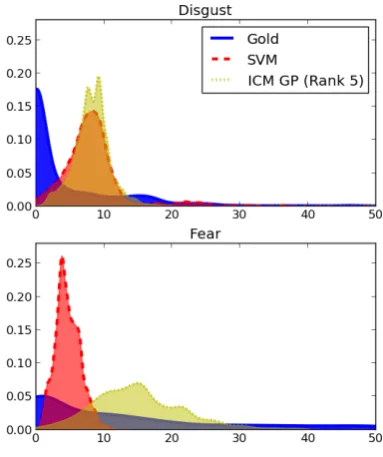
To check why SVM performs better than GPs for some emotions, we analysed their gold-standard score distributions. Figure 2 shows the smoothed distributions fordisgust and fear, comparing the gold-standard scores to predictions from the SVM and GP models. The distributions for the training set follow similar shapes.
We can see that GP obtains better matching score distributions in the case when the
gold-Figure 2: Test score distributions for disgust and
fear. For clarity, only scores between 0 and 50 are shown. SVM performs better ondisgust, while GP performs better onfear.
[image:4.595.317.509.242.471.2]more narrow coverage of the SVM.
More importantly, Figure 2 also shows that both SVM and GP predictions tend to exhibit a Gaus-sian shape, while the true scores show an expo-nential behaviour. This suggests that both mod-els are making wrong prior assumptions about the underlying score distribution. For SVMs, this is a non-trivial issue to address, although it is much easier for GPs, where we can use a different like-lihood distribution, e.g., a Beta distribution to re-flect that the outputs are only valid over a bounded range. Note that non-Gaussian likelihoods mean that exact inference is no longer tractable, due to the lack of conjugacy between the prior and likeli-hood. However a number of approximate infer-ence methods are appropriate which are already widely used in the GP literature for use with non-Gaussian likelihoods, including expectation prop-agation (Jyl¨anki et al., 2011), the Laplace approx-imation (Williams and Barber, 1998) and Markov Chain Monte Carlo sampling (Adams et al., 2009).
4.4 Training Set Influence
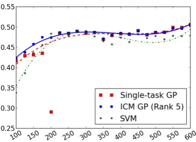
We expect multi-task models to perform better for smaller datasets, when compared to single-task models. This stems from the fact that with small datasets often there is more uncertainty associated with each task, a problem which can be alleviated using statistics from the other tasks. To measure this behaviour, we performed an additional exper-iment varying the size of the training sets, while using100sentences for testing.
Figure 3 shows the scores obtained. As ex-pected, for smaller datasets the single-task mod-els are outperformed by ICM, but their perfor-mance become equivalent as the training set size increases. SVM performance tends to be slightly worse for most sizes. To study why we obtained an outlier for the single-task model with200 sen-tences, we inspected the prediction values. We found that, in this case, predictions for joy, sur-priseanddisgustwere all around the same value.6 For larger datasets, this effect disappears and the single-task models yield good predictions.
5 Conclusions and Future Work
This paper proposed an multi-task approach for Emotion Analysis that is able to learn correlations
6Looking at the predictions for smaller datasets, we found
[image:5.595.319.510.71.209.2]the same behaviour, but because the values found were near the mean they did not hurt the Pearson’s score as much.
Figure 3: Pearson’s correlation score according to training set size (in number of sentences).
and anti-correlations between emotions. Our for-mulation is based on a combination of a Gaussian Process and a low-rank coregionalisation model, using a richer parameterisation that allows the learning of fine-grained task similarities. The pro-posed model outperformed strong baselines when applied to a news headline dataset.
As it was discussed in Section 4.3, we plan to further explore the possibility of using non-Gaussian likelihoods with the GP models. An-other research avenue we intend to explore is to employ multiple layers of metadata, similar to the model proposed by Cohn and Specia (2013). An example is to incorporate the dataset provided by Snow et al. (2008), which provides multiple non-expert emotion annotations for each sentence, ob-tained via crowdsourcing. Finally, another possi-ble extension comes from more advanced vector-valued GP models, such as the linear model of coregionalisation ( ´Alvarez et al., 2012) or hierar-chical kernels (Hensman et al., 2013). These mod-els can be specially useful when we want to em-ploy multiple kernels to explain the relation be-tween the input data and the labels.
Acknowledgements
Daniel Beck was supported by funding from CNPq/Brazil (No. 237999/2012-9). Dr. Cohn is the recipient of an Australian Re-search Council Future Fellowship (project number FT130101105).
References
Inference in Poisson Processes with Gaussian Pro-cess Intensities. InProceedings of ICML, pages 1–8, New York, New York, USA. ACM Press.
Mauricio A. ´Alvarez, Lorenzo Rosasco, and Neil D. Lawrence. 2012. Kernels for Vector-Valued Func-tions: a Review. Foundations and Trends in Ma-chine Learning, pages 1–37.
Daniel Beck, Kashif Shah, Trevor Cohn, and Lucia Specia. 2013. SHEF-Lite : When Less is More for Translation Quality Estimation. InProceedings of WMT13, pages 337–342.
Steven Bird, Ewan Klein, and Edward Loper. 2009. Natural Language Processing with Python. O’Reilly Media.
Edwin V. Bonilla, Kian Ming A. Chai, and Christopher K. I. Williams. 2008. Multi-task Gaussian Process Prediction. Advances in Neural Information Pro-cessing Systems.
Rich Caruana. 1997. Multitask Learning. Machine Learning, 28:41–75.
Trevor Cohn and Lucia Specia. 2013. Modelling Annotator Bias with Multi-task Gaussian Processes: An Application to Machine Translation Quality Es-timation. InProceedings of ACL.
Hal Daum´e III. 2007. Frustratingly easy domain adap-tation. InProceedings of ACL.
Jenny Rose Finkel and Christopher D. Manning. 2009. Hierarchical Bayesian Domain Adaptation. In Pro-ceedings of NAACL.
James Hensman, Neil D Lawrence, and Magnus Rat-tray. 2013. Hierarchical Bayesian modelling of gene expression time series across irregularly sam-pled replicates and clusters. BMC Bioinformatics, 14:252.
Pasi Jyl¨anki, Jarno Vanhatalo, and Aki Vehtari. 2011. Robust Gaussian Process Regression with a Student-t Likelihood. Journal of Machine Learning Re-search, 12:3227–3257.
Rada Mihalcea and Carlo Strapparava. 2012. Lyrics, Music, and Emotions. InProceedings of the Joint Conference on Empirical Methods in Natural guage Processing and Computational Natural Lan-guage Learning, pages 590–599.
Bo Pang and Lillian Lee. 2008. Opinion Mining and Sentiment Analysis. Foundations and Trends in In-formation Retrieval, 2(1–2):1–135.
Fabian Pedregosa, Ga¨el Varoquaux, Alexandre Gram-fort, Vincent Michel, Bertrand Thirion, Olivier Grisel, Mathieu Blondel, Peter Prettenhofer, Ron Weiss, Vincent Duborg, Jake Vanderplas, Alexan-dre Passos, David Cournapeau, Matthieu Brucher, Matthieu Perrot, and ´Edouard Duchesnay. 2011. Scikit-learn: Machine learning in Python. Journal of Machine Learning Research, 12:2825–2830.
Daniel Preotiuc-Pietro and Trevor Cohn. 2013. A tem-poral model of text periodicities using Gaussian Pro-cesses. InProceedings of EMNLP.
Carl Edward Rasmussen and Christopher K. I. Williams. 2006. Gaussian processes for machine learning, volume 1. MIT Press Cambridge.
Kashif Shah, Trevor Cohn, and Lucia Specia. 2013. An Investigation on the Effectiveness of Features for Translation Quality Estimation. InProceedings of MT Summit XIV.
Rion Snow, Brendan O’Connor, Daniel Jurafsky, and Andrew Y. Ng. 2008. Cheap and Fast - But is it Good?: Evaluating Non-Expert Annotations for Natural Language Tasks. In Proceedings of EMNLP.
Carlo Strapparava and Rada Mihalcea. 2007. SemEval-2007 Task 14 : Affective Text. In Pro-ceedings of SEMEVAL.
Carlo Strapparava and Rada Mihalcea. 2008. Learning to identify emotions in text. InProceedings of the 2008 ACM Symposium on Applied Computing. Christopher K. I. Williams and David Barber. 1998.