Scholarship@Western
Scholarship@Western
Electronic Thesis and Dissertation Repository
2-13-2018 2:30 PM
Modelling the Common Risk among Equities Using a New Time
Modelling the Common Risk among Equities Using a New Time
Series Model
Series Model
Jingjia ChuThe University of Western Ontario Supervisor
Kulperger, Reg
The University of Western Ontario Joint Supervisor Yu, Hao
The University of Western Ontario
Graduate Program in Statistics and Actuarial Sciences
A thesis submitted in partial fulfillment of the requirements for the degree in Doctor of Philosophy
© Jingjia Chu 2018
Follow this and additional works at: https://ir.lib.uwo.ca/etd
Part of the Longitudinal Data Analysis and Time Series Commons, Multivariate Analysis Commons, Statistical Models Commons, and the Statistical Theory Commons
Recommended Citation Recommended Citation
Chu, Jingjia, "Modelling the Common Risk among Equities Using a New Time Series Model" (2018). Electronic Thesis and Dissertation Repository. 5223.
https://ir.lib.uwo.ca/etd/5223
This Dissertation/Thesis is brought to you for free and open access by Scholarship@Western. It has been accepted for inclusion in Electronic Thesis and Dissertation Repository by an authorized administrator of
A new additive structure of multivariate GARCH model is proposed where the
dy-namic changes of the conditional correlation between the stocks are aggregated by the
common risk term. The observable sequence is divided into two parts, a common risk
term and an individual risk term, both following a GARCH type structure. The
condi-tional volatility of each stock will be the sum of these two condicondi-tional variance terms.
All the conditional volatility of the stock can shoot up together because a sudden peak
of the common volatility is a sign of the system shock.
We provide sufficient conditions for strict stationarity and ergodicity of the model.
The ergodicity of the model cannot be studied in the standard way because of the
non-linearity. After reforming the original mathematical representation of the model into a
complicated Markovian structure, the systematic theory for Markov chain from Meyn
and Tweedie (2009) is applied.
All the parameters in the model are identifiable in terms of the second conditional
moments under mild assumptions. Then there exists a unique solution of parameters in
the domain which maximizes the likelihood function for a sufficiently large sample size.
The choice of starting values is unimportant within the parameter space defined by the
ergodicity theorem. Under some general assumptions we proposed, without specifying
the distribution of the innovation, different initial values will lead to the same estimates
asymptotically. Once both assumptions for ergodicity and identifiability are satisfied,
the quasi maximum likelihood (QML) has become a reasonable method to estimate
pa-rameters in practice. The sufficient conditions for the strong consistency and asymptotic
normality of the QML estimator are proposed.
The Monte Carlo simulation example is included in this thesis to demonstrate how to
verify the assumptions in the strict stationarity and asymptotic normality theorems. The
numeric issues for the estimating process in practice are addressed with possible solutions.
ity, GARCH, Multivariate Time Series, Underlying Driven Process, Asymptotic
Normal-ity, Consistency.
The research included in this dissertation could not have been performed without the
assistance and support of many individuals. I would like to extend my gratitude first and
foremost to my thesis supervisors, Dr. Reg Kulperger and Dr. Hao Yu, for mentoring me
over my Ph.D. research. Their everlasting patience, academic enthusiasm, and immense
knowledge sustain the cumulative progress of my research. Their guidance helped me in
all the time of my study and work.
I would like to take this opportunity to thank my examiners: Dr. Adam Kolkiewicz,
Dr. Stephen Sapp, Dr. Marcos Escobar-Anel and Dr. Rogemar Mamon for their
willing-ness and effort to my defense.
I am grateful for the advice I received from Dr. Duncan Murdoch during my Master’s
program. I am also indebted to my instructors at the University of Western Ontario,
including but not limited to Dr. John Braun, Dr. Ian McLeod, Dr. Wenqing He,
Dr. David Stanford and Dr. Mark Reesor. It was them who showed me the path into
the kingdom of statistics when I started my graduate study. I also want to convey my
appreciation to my mentors of statistical consultation, Dr. David Bellhouse and Dr.
Bethany White. Their encouragement and assistance are highly appreciated and will
always be remembered.
Besides that, I would also like to extend my deepest gratitude to my parents,
grand-parents and Tianwei without whose love, support, and understanding I could never have
completed this doctoral degree.
Last but not least, I would like to thank all my friends and colleagues, Na Li, Bin
Luo, Xin Liu, Xin Wang, Jiang Wu, Yaofei Xiong, Yuzhou Zhang, Heng Xiong, Shen
Shan, Chen Yang and others.
Special thanks to two of my non-human friends, Bilbo and Rosie. They have been
playing a very important role during my journey at Western.
Abstract i
Dedication iii
Acknowlegements iv
List of Figures vii
List of Tables ix
1 Introduction 1
1.1 Heteroskedasticity Models . . . 3
1.2 Factor models . . . 8
1.3 Model Specification . . . 11
1.4 Statistical Theory of multivariate models . . . 16
1.5 Organization of the Thesis . . . 18
2 Ergodicity and Stationarity 19 2.1 Introduction . . . 19
2.2 Markovian Process and Nonlinear State Space Model . . . 22
2.3 Ergodicity and Stationarity Theorem . . . 26
2.4 Proof of the Theorem . . . 28
3 Gaussian QMLE and its Asymptotic Theory 38 3.1 Gaussian Quasi-Maximum Likelihood Estimator . . . 38
3.2.1 Proof of Theorem 3.2.2 . . . 44
3.2.2 Lemmas . . . 46
3.3 Asymptotic Normality . . . 61
3.3.1 Proof of Theorem 3.3.1 . . . 62
3.3.2 Lemmas . . . 72
4 Simulation Study 114 4.1 Introduction . . . 114
4.2 Monte Carlo Study Preparation . . . 115
4.3 Simulated Results . . . 119
4.4 Numeric Issues with Solutions . . . 129
4.4.1 The Scale Difference . . . 129
4.4.2 Computational Speed . . . 134
4.4.3 Initial values and Starting Point . . . 135
5 Concluding Remarks 140
Bibliography 142
A Useful algebra results 149
B Some Definitions in Markov Chain 152
C Other Mathematical definitions 154
Curriculum Vitae 155
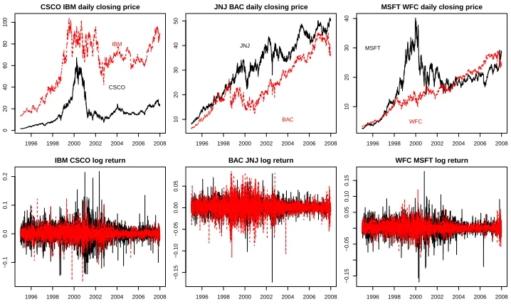
1.1 The original daily closing prices and the log returns . . . 2
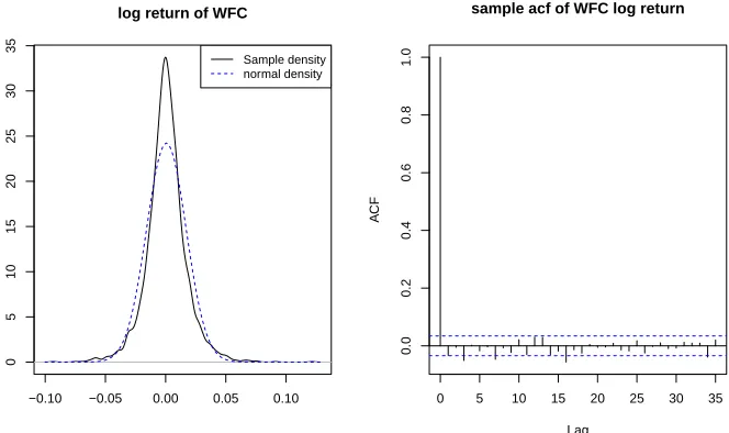
1.2 The plot on the left: the solid black line shows the sample density of WFC
log return, the blue dashed line shows the corresponding normal density.
The plot on the right: the sample autocorrelation of WFC log return. . . 3
1.3 The sample autocorrelation plots of transformed WFC log returns
(abso-lute values on the left and squared values on the right). . . 4
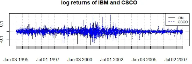
4.1 Log return of IBM and CSCO from 1995-01-01 to 2007-12-31 . . . 116
4.2 The simulated paths: the top three are the simulated xt (the black solid
line represents x1,t and the red dashed line represents x2,t) and the three
below are the correspondingσt (the black line representsσ21,t, the red line
representsσ2
2,t and the blue line representsσ
2
0,t) . . . 121
4.3 The histogram of αˆ1,αˆ2,βˆ1,βˆ2 when K2 = 1000. The blue lines represent
the true values. . . 121
4.4 The histogram of ρ,ˆ ωˆ1,ωˆ2,βˆ0 when K2 = 1000. The blue lines represent
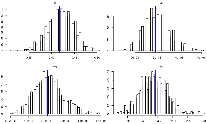
the true values. . . 122
4.5 The histogram ofαˆ1,αˆ2,βˆ1,βˆ2 when K2 = 20000. The blue lines represent
the true values. . . 122
4.6 The histogram of ρ,ˆ ωˆ1,ωˆ2,βˆ0 when K2 = 20000. The blue lines represent
the true values. . . 123
4.7 qqnorm of rescaledρ1,2ˆ with different sample sizes K2 . . . 129
4.8 qqnorm of rescaledωˆ1 with different sample sizes K2 . . . 130
4.10 qqnorm of rescaled βˆ0 with different sample sizes K2 . . . 131
4.11 The black solid line: kernel density of rescaled ρˆ1,2 with different sample
sizes K2. The blue dashed line: standard normal using the same mean and
sd from the estimates . . . 131
4.12 The black solid line: kernel density of rescaled ωˆ1 with different sample
sizes K2. The blue dashed line: standard normal using the same mean and
sd from the estimates . . . 132
4.13 The black solid line: kernel density of rescaled βˆ1 with different sample
sizes K2. The blue dashed line: standard normal using the same mean and
sd from the estimates . . . 132
4.14 The black solid line: kernel density of rescaled βˆ0 with different sample
sizes K2. The blue dashed line: standard normal using the same mean and
sd from the estimates . . . 133
4.15 Violin plot for 1000 computation time using the same target function
writ-ten in R and Rcpp . . . 136
4.1 The numeric estimate from IBM and CSCO centered log return and the
‘True’ value used for the bootstrap simulations (rounded to two decimal
digits) . . . 119
4.2 The absolute biases with different sample sizes (rounded to two decimal
digits) . . . 125
4.3 The relative absolute biases with different sample size (%) . . . 125
4.4 RMSE of the estimates (rounded to two decimal digits) . . . 126
4.5 SD of √K2(ˆθK2−θ0)and estimated asymptotic SD (rounded to two decimal
digits) . . . 128
4.6 RASY with different sample sizes (%) . . . 128
4.7 Kurtosis (skewness) of √K2(ˆθK2 −θ0) (rounded to one decimal digits) . . 133
4.8 Estimates and corresponding values of the negative likelihood from
Win-dows and Linux system: θˆ1 is the estimate from Windows system and θˆ2
is the estimate from Windows system. . . 137
4.9 Estimates and corresponding values of the negative likelihood from
Win-dows and Linux system usingθstart,a and θstart,b. . . 138
Introduction
The log returns are commonly used in econometrics for some reasons. The raw prices are
restricted to be positive whereas the log returns can be any real numbers. Let S0,S1, . . .
be a sequence of daily stock closing prices. Then the log return xt (or return in the
following sections) is defined as
xt = log(St/St−1)≈
St −St−1
St−1
.
The right hand side of the approximation sign is obtained by Taylor expansion. The
log returns can be interpreted as continuously compounded returns and the log return
values do not depend on monetary units of the original asset prices (see Figure 1.1 and
4.1). Moreover, the weekly or monthly log returns can be easily computed by summing
up the daily returns. Most of the observations plotted in Figure 4.1 fall into a relatively
narrow range with only few above 5% or below -5%.
As a measure of riskiness in financial securities, it is necessary to estimate the volatility
of the log returns instead of the raw prices for the financial modeling. Though the
volatility of the log returns does not tell which direction the log return goes, it can tell
us how far on average the returns move. It can be used in derivative pricing and risk
control.
1996 1998 2000 2002 2004 2006 2008
0
20
40
60
80
100
CSCO IBM daily closing price
CSCO IBM
1996 1998 2000 2002 2004 2006 2008
−0.1
0.0
0.1
0.2
IBM CSCO log return
1996 1998 2000 2002 2004 2006 2008
10
20
30
40
50
JNJ BAC daily closing price
JNJ
BAC
1996 1998 2000 2002 2004 2006 2008
−0.15
−0.10
−0.05
0.00
0.05
BAC JNJ log return
1996 1998 2000 2002 2004 2006 2008
10
20
30
40
MSFT WFC daily closing price
MSFT
WFC
1996 1998 2000 2002 2004 2006 2008
−0.15
−0.05
0.05
0.10
0.15
WFC MSFT log return
Figure 1.1: The original daily closing prices and the log returns
In early studies of financial models, the log returns are assumed to be independent
and identically distributed with a mean and a variance which remain the same over time.
This type of structure is motivated by the Black-Scholes-Merton (BSM) model (Black
and Scholes, 1973; Merton, 1973) which is an important framework to derive the option
prices. In the BSM model,
dSt/St =µdt+σdWt.
After discretizing the time interval in this formula, this formula leads to the conclusion
that the daily log returns follow an independent and identically normal distribution with
mean (µ− 1 2σ
2) and variance σ2. Therefore, the volatility of the log returns can be
estimated by the sample standard deviation. If x¯= 1 n
Pn
i=1xi, then
σ=
v t
1 n
n
X
i=1
(xi −x)¯ 2.
Such an assumption does not hold in practice for all kinds of different reasons. If
the log returns are normally distributed, the sample density will be close to the normal
−0.10 −0.05 0.00 0.05 0.10
0
5
10
15
20
25
30
35
log return of WFC
Sample density normal density
0 5 10 15 20 25 30 35
0.0
0.2
0.4
0.6
0.8
1.0
Lag
A
CF
sample acf of WFC log return
Figure 1.2: The plot on the left: the solid black line shows the sample density of WFC log return, the blue dashed line shows the corresponding normal density. The plot on the right: the sample autocorrelation of WFC log return.
compared to the corresponding theoretical normal density. This phenomenon is known
as leptokurtosis. Another noticeable violation is that a large value tends to be followed
by another large value, and a small value tends to be followed by another small value,
regardless of signs. This characteristic of financial time series is called volatility clustering.
One more evidence of such a feature is based on the sample autocorrelation functions.
Though the sample autocorrelations of the log return sequence are mostly within the
confidence bands around 0, the sample autocorrelations of the transformed sequences,
both the absolute values and the squared values, decay to 0 slowly in Figures 1.2 and 1.3.
All of these suggest that the second order of the log returns or volatilities is changing
dynamically depending on the previous values.
1.1
Heteroskedasticity Models
The conditional heteroskedasticity models have played an important role in financial
0 5 10 15 20 25 30 35
0.0
0.2
0.4
0.6
0.8
1.0
Lag
A
CF
sample acf of absolute log return
0 5 10 15 20 25 30 35
0.0
0.2
0.4
0.6
0.8
1.0
Lag
A
CF
sample acf of squared log return
Figure 1.3: The sample autocorrelation plots of transformed WFC log returns (absolute values on the left and squared values on the right).
Assume {xt : t > 0} is the observed process and let Ft be a set (σ-field) generated by
{xt,xt−1, . . .}, then the general form of the conditional heteroskedasticity model is written
in a multiplicative structure. The variance of the log return depends on the observations
up to one-step before the current time. In mathematical equations,
xt =tσt
E(xt|Ft−1)=0
E(x2t|Ft−1)=σ2t .
(1.1)
The innovations{t :t∈T}are i.i.d. random noise with mean 0 and variance 1. Moreover,
the innovations are independent ofFt−1, and σt’s are Ft−1 adapted.
Engle (1982) introduced the autoregressive conditional heteroskedasticity (ARCH)
model with the unique ability of capturing volatility clustering in financial time series at
the time. The ARCH(q) model defines the conditional variance of xt to be
σ2
t = ω+ q
X
i=1
However, the selected lag q tends to be large when the model is applied to real market
data. Subsequently, Bollerslev (1986) extended the formula of σ2
t by adding its
autore-gressive terms, then the number of terms on the right hand side can be notably reduced.
The conditional variance of the univariate GARCH(p,q) model is defined as
σ2
t = ω+ q
X
i=1
αix2t−i+ p
X
j=1
βjσ2t−j.
If the backshift operator is used in the representation, the univariate GARCH(p,q) model
can be written as an ARCH(∞) model. The ARCH(∞) model is
σ2
t =φ0+
∞
X
i=1
φit2−i.
The detailed equalities of the coefficients can be found in Francq and Zakoian (2010).
Other extensions of the univariate GARCH model try to characterize the
asymme-try effect, which include exponential GARCH model (Nelson, 1991), threshold GARCH
model (Zakoian, 1994), double threshold (G)ARCH model (Li and Li, 1996), dynamic
asymmetric GARCH model (Caporin and McAleer, 2006). The theories and applications
of univariate (G)ARCH type models are well developed, while the multivariate cases are
much harder in general.
When there is more than one time series, it becomes necessary to understand the
co-movements of the returns. It is well known that the volatilities of stock returns are
correlated with each other. In contrast to the univariate cases, the multivariate volatility
estimations based on a GARCH dependence are much more flexible. There are two
possible ways to build a parametric model in the multivariate GARCH models. One
is to model the conditional second moment directly and the other one is to model the
conditional correlation along with the marginal conditional variance for each sequence
together.
moments as well as the univariate cases. A multivariate volatility model, called half-Vec
(vech) GARCH model (Bollerslev et al., 1988), is also one of the most general forms of
multivariate GARCH models. Let vechdenote the vector-half operator, which stacks the
lower triangular elements of anm×mmatrix as a vector with lengthm×(m+1)/2. Then
xt =Ht1/2t,
ht = c+
q
X
i=1
Aiηt−i+
p
X
j=1
Bjht−j,
(1.2)
where
ht = vech(Ht),
ηt−i = vech(tt|),
t i.i.d.∼ (0,Im),
and Ai, Bj are m×m coefficient matrices.
In this class of models, the conditional covariance matrix is modeled directly. The
number of parameters in the generalm-dimensional case is
(p+q)
"
m(m+1) 2
#2
+ m(m+1)
2
.
It increases at a rate proportional to m4, which makes it difficult to get the estimations.
Another famous class of the multivariate GARCH models built on Ht is the BEKK
model (Bollerslev et al., 1988; Engle and Kroner, 1995). The conditional covariance
matrix is considered as
Ht =CC|+ K
X
k=1
q
X
i=1
Aiktt|A|ik+ K
X
k=1
p
X
i=1
BikHt−iB|ik
where C, Aik and Bik are m bym matrices. C is a triangular matrix, Aik and Bik are not
necessarily symmetric. The number of parameters is (p+q)Km2 + m(m+1)
2 , which is much smaller than theVech version.
mentioned above. The constant correlation coefficient (CCC) GARCH model is presented
by Bollerslev (1990), who assumes that the conditional correlation matrix R is
time-invariant, where
R=
1 ρ1,2 . . . ρ1,m
ρ1,2 1 . . . ρ2,m
... ... ... ... ρ1,m ρ2,m . . . 1
m×m
The number of parameters is reduced to O(m2) from O(m4) in theVech GARCH model.
The model is defined as
xt = Ht1/2t,
Ht =StRSt,
∆t =c+
q
X
i=1
Aixt−i2+
p
X
j=1
Bj∆t−j,
(1.3)
where ∆t is a m dimensional vector of diagonal elements of the conditional covariance
matrix Ht, St is the diagonal matrix of the elements in √
∆t, and the square vector xt−i2
is (x2
1,t−i,· · · ,x
2
m,t−i)|.
A less restrictive time-variant conditional correlation version, called the dynamic
cor-relation coefficient (DCC) GARCH, is studied by Engle (2002), Tse and Tsui (2002).
The conditional correlation is changed to be dynamic in the structure of Ht.
Ht =StRtSt
where the elements in Rt, ρi j,t =
qi j,t √
qii,tqj j,t
. The terms in both the denominator and the
numerator can be written as a weighted average of their past values and the element in
matrix tt|, may or may not with a constant. In matrix form,
or
Qt =S(1−α−β)+α(tt|)+βQt−1.
Both CCC-GARCH and DCC-GARCH models are built by modelling the conditional
variance of each series and the conditional correlation between series.
There are additional extensions to the multivariate GARCH models as described
above, e.g. the generalized orthogonal GARCH (Van der Weide, 2002) and the vector
ARMA-GARCH model (Ling and McAleer, 2003).
1.2
Factor models
The strong positive association between the equity variance and several explanatory
vari-ables is confirmed by Christie (1982). The volatilities of equities are driven by the same
underlying process which is related to some variables besides the returns. A successful
class of the multivariate models is the capital asset model and its extension, factor
mod-els. The asset pricing model (Treynor, 1962, 1961; Sharpe, 1964) has been introduced by
economists by comparing the sensitivity, β’s, of the series with the overall market risk.
Later, Fama and French expanded the variables in the asset returns model to a three
factor model (Fama and French, 1993) and a five factor model (Fama and French, 2015).
In the earliest setup, there is only one factor which is the market return. The model is
Exi = xf +βi(Exm− xf)
where xi is the return of asseti, xf is the risk-free rate of interest and βi is the sensitivity
of the expected excess asset returns to the expected excess market returns. In such a
setup, the correlation between two expected returns, ρi,j = βiβj, is a constant over time.
These models only consider the relative risk between the individual series and the general
the common risk factors which do not take the dynamic change along with time into
consideration.
One way to improve the model is to change the static factors into hidden dynamic
factors. The generalized factor model (Forni et al., 2000) assumes the individual log
return is a linear combination of K factors with an idiosyncratic risk,
xi,t = K
X
j=1
βjft,j+ηi,t, i= 1,2, . . . ,m.
or in a matrix form
xt = Bft+ηt
where B is a loading matrix withmrows and K columns, the idiosyncratic risk are
corre-lated with a covariance matrixΩ. The factors have the following conditional specification
Et−1(ft)=0,
Et−1(ftft|)= Λt where Λt is a positive definite matrix.
The conditional covariance matrix of xt is
Ht = BΛtB| + Ω.
The identifiability in the dynamic factor models is a problem since any full rank square
matrix T can be used to premultiply the factor ft, then the conditional second moment
remains the same which means
Ht =(BT)(T−1Λt(T|)−1)(BT)|.
moment. The number of parameters increases at a rate proportional to m2 because the
number of elements in Bis m(m+1)/2.
The factor GARCH model (Vrontos et al., 2003) is a special case of the factor model
with Ω =0 and the number of factors equals to the dimensions of the observed process,
K = m. Moreover,Λt is assumed to be a diagonal matrix with GARCH specified diagonal
elements σ2
i,t where
σ2
i,t =ωi+αifi2,t−1+βiσ2i,t−1, i=1, . . . ,m.
Hafner and Preminger (2009a) solve the identification problem by putting constraints on
the constant terms ωi’s in the GARCH structure such that all of them are set to be one
in the equation above.
Though the dynamic factor model has many good features, it has some problems in
practice. In the general dynamic factor model settings, the number of factors K need to
be specified at the beginning (see Hallin and Liˇska, 2007). As in the principal component
analysis, the factors may lack practical interpretations.
Another way to improve the static factor model is to build the model with economic
reasoning. The risk can be divided in to systematic and idiosyncratic risk factors with
an additive structure. Using the idea from Vasicek (1987),
xi,t = ρi0,t+
q
1−ρ2
ii,t
where 0,t is the systematic risk and i,t’s are the idiosyncratic risks. The systematic risk
and each of the idiosyncratic risks are independent of each other. In this setting, the
correlation between assets i and j remains constant over time, which is ρiρj. Berd et al.
(2007) modified the model into a one-factor (G)ARCH model that
whereb≥0andr0,t is the market risk factor (systematic risk). The market risk factorr0,t
has a conditional distribution with mean 0 and variance σ2
0,t, whereσ
2
0,t has the structure
of a univariate GARCH conditional variance. The model has been introduced without
any statistical property.
Generally speaking, the factor models with loading matrices have identifiability
prob-lem. If the conditional distribution of the factors remains the same over time (e.g. the
constant conditional mean and variance), then the loadings can be simply determined
by the unique solution of a linear regression. However, if the conditional distribution of
the factors is changing dynamically, the number of solutions of the loading matrix can
be infinity without additional constraints.
1.3
Model Specification
With information flowing around the world instantaneously, most markets (Asian,
Euro-pean, and American) will react to the same events (good news or bad news). Currently,
most stock prices will go up or down together following big events (random shocks).
Carr and Wu (2009) found that a common stochastic variance risk factor exists among
the stocks by using the market option premiums. We want to introduce a simple common
risk model which keeps the GARCH structure and involves the stock returns only. We
propose a new additive GARCH type model by using a common risk term to characterize
the internal relationship among series explicitly. The common risk term could be used as
an indicator of the shock among series. The conditional correlations aggregated by this
common risk term are changing dynamically.
The univariate GARCH model has a huge success in financial practice, while most
of the multivariate GARCH models extensions do not have a simple way to capture the
common risk among different stocks. The goal of this section is to propose a model which
similar to the univariate GARCH model, and it will also have characteristics similar to
the univariate GARCH model. The idea is borrowed from the factor models to use an
additive structure. Not like the class of DCC GARCH models, asymptotic theorems can
be provided in this new setting.
Some empirical studies show that GARCH model with p = q = 1 is the most
com-monly used one in applied econometrics, so we only define the model as an extension of
GARCH(1,1) process here. The model could be easily generalized based on GARCH(p,q)
case, although the statistical study of the generalized model will be much harder.
Consider an Rm-valued stochastic process {x
t,t ∈Z} on a probability space (Ω,A,P)
and a multidimensional parameterθ in the parameter space Θ where
θ= (ρ1,2,· · · , ρm−1,m, ω1,· · · , ωm, α1,· · · , αm, β1,· · · , βm, β01,· · · , β0m)|,
which belongs to a parameter space of the form
Θ⊂ [−1,1]m(m2−1) ×[0,∞)4m.
Denote a m+1 dimensional real valued innovation process by {t,t ∈ Z}, and the
infor-mation set (σ-field) denote the information set available at time t byFt = σ(t,t−1, . . .).
Assume that the innovations are independent and identically distributed with mean 0
and covariance matrix Σ which is also a correlation matrix,
Σ =
Rm×m 0m×1
01×m 1
where R is the same matrix defined above. The elements in the R matrix represent the
internal connections between shocks. When R is an identity matrix, the model becomes
a two factor model with the loading coefficients set to be 1.
t,ind=(1,t, 2,t, . . . , m,t)|.The first part is an m-dimensional vector of correlated individual
shocks t,ind and the second part is a univariate independent common shock term 0,t.
We say that xt is a common risk model with an additive GARCH structure if, for all
t∈Z, we have
x1,t = 1,tσ1,t+0,tσ0,t
x2,t = 2,tσ2,t+0,tσ0,t
· · · ·
xm,t = m,tσm,t +0,tσ0,t
(1.4)
where σ1,t, . . . , σm,t are following a GARCH structure and σ0,t is related to all of them,
σ2
1,t = ω1+α1x1,2t−1+β1σ21,t−1
σ2
2,t = ω2+α2x2,2t−1+β2σ22,t−1
· · · ·
σ2
m,t = ωm+αmx2m,t−1+βmσ2m,t−1
σ2
0,t = β01σ21,t+· · ·+β0mσ2m,t.
(1.5)
Introduce the following notations,
Dt =diag{σ1,t, σ2,t· · · , σm,t},1=(1,1,· · · ,1)|.
Then (1.4) could be written in a matrix form:
xt = Dtt,ind+σ0,t0,t1. (1.6)
So the model could either be specified by (1.5) and (1.6) together or (1.4) and (1.5)
together.
The main idea of this setup has been published in Chu et al. (2016) but in a slightly
also included in that proceeding manuscript without proof, whereas this thesis gives
additional details. Aside from the reason to obtain the parameter identifiability, the
structure of the covariance matrixΣ has its own interpretation. For a bivariate case, this
model allows two stock returns to be correlated through the individual innovations even
in the absence of the common shock. An independent external shock is applied to the
two stocks in the same way which drives the returns simultaneously.
The number of parameters is increasing at the rate O(m2) which is similar to the
CCC-GARCH model. We could partition the vector of unknown parameters into two
parts: the parameters in the innovations correlation matrix Σ and the coefficients in
(1.5). The number of total parameters is s = s1 +3m+1, where s1 =
m(m−1)
2 is the number of parameters in R. There is no redundancy in defining the dependency among
the returns through the matrixΣ and the common factor σ2
0,t in the model. The process
is the same as a CCC-GARCH(1,1) process when β01 = β02 = · · · = β0m = 0. Therefore,
CCC-GARCH(1,1) is a special case of this process. Note that for ρ1,2 = · · ·= ρm−1,m =0, the process further reduces to m independent univariate GARCH(1,1) series.
The conditional covariance matrix of xt, Ht =cov(xt|Ft−1), can be computed from the
definition,
Ht =
σ2 0,t +σ
2
1,t σ
2
0,t+ρ1,2σ1,tσ2,t . . . σ
2
0,t +ρ1,mσ1,tσm,t
σ2
0,t+ρ1,2σ1,tσ2,t σ
2 0,t+σ
2
2,t . . . σ
2
0,t +ρ2,mσ2,tσm,t
... ... ... ...
σ2
0,t+ρ1,mσ1,tσm,t σ
2
0,t +ρ2,mσ2,tσm,t . . . σ
2 0,t+σ
2
m,t
.
Ht can be written as the sum of two parts: Ht = σ2
0,tJ+DtRDt where
J =
1 1 . . . 1
... ... ... ...
1 1 . . . 1
m×m
Each term on the left hand side (1.5) has its own lower bound,
σ2
1,t ≥ ω1, . . . , σ2m,t ≥ ωm and σ0,2t ≥β01ω1+· · ·+β0mωm.
Hence, the conditional variance of each component in xt at time t has different lower
bound as well.
The conditional correlation between series i and series j can be represented by the
elements in Ht matrix
ρi j,t =
cov(xi,t,xj,t)
p
var(xi,t) var(xj,t)
= σ
2
0,t+ρi,jσi,tσj,t
q
(σ2 0,t+σ
2
i,t)(σ
2 0,t +σ
2
j,t)
=
1+ρi,j
σi,t
σ0,t
σj,t
σ0,t
v u u u u u u t
1+
σi,t
σ0,t
2vu u u u u u t
1+
σj,t
σ0,t
2.
From the equations above, the conditional correlation matrix tends to be J when the
common term σ0,t is much larger than both σi,t and σj,t. In this case, the common risk
term is dominant, and all the log return series are nearly perfectly correlated. On the
contrary, the conditional correlation matrix will be approaching the constant correlation
matrix R when the common risk term is much smaller thanσi,t and σj,t or is really close
to 0. Then, the conditional correlation will become time invariant which is the same as
a CCC-GARCH model. Mathematically,
Rt → J when σ0,t → ∞,
Based on the specification in (1.5), Rt cannot be neither J or R as σ2
0,t is a linear
com-bination of σ2
i,t for i = 1,2,· · · ,m. Nonetheless, the expression for σ
2
0,t can have other
possibilities which might involve terms like σ2 0,t−1, x
2
i,t−1 or σ 2
i,t−1. This is only a
demon-stration of the potential of the model with the additive structure in (1.4).
1.4
Statistical Theory of multivariate models
Since the model proposed in the previous section follows a GARCH type structure, the
main tool used in this thesis can be borrowed from the GARCH models. The theories in
this thesis include the stationarity and ergodicity theorem, the consistency theorem and
the asymptotic normality theorem.
The strict stationarity of the univariate GARCH(1,1) model is proved in Kl¨uppelberg
et al. (2004) by rewriting the conditional variance σ2i,t as an infinite sum of the past
squared innovations {t2}. Whether the process is strictly stationary depends on γ where
γ =Elogαη2t +β. The necessary and sufficient conditions for a univariate GARCH(p, q)
model is provided in Nelson and Cao (1992) and Tsai and Chan (2008). In the general
univariate GARCH (p,q), the latest pconditional variance can be combined with the last
qobserved points to construct a linear representation in vector form. The top Lyapunov
exponent of the spectral radius of the coefficient matrix in the new form is used to control
the strong consistency.
The local consistency and asymptotic normality theorem of the QMLE in the
uni-variate GARCH(1,1) model is provided in Lumsdaine (1996). A local neighbourhood of
the true parameter is defined, then the consistency theorem is built inside this
neigh-bourhood under very restrictive assumptions. Lee and Hansen (1994) provide the strong
consistency among the whole parameter space in the univariate GARCH(1,1) setting
un-der the strictly stationary and ergodic assumption. The finite moment requirement is
and asymptotic normality theorems in a univariate GARCH(p,q) model is very similar to
the GARCH(1,1) case which uses the top Lyapunov exponent and the finite 4th moment
plus some other conditions (see Berkes et al., 2003; Francq and Zako¨ıan, 2004).
The theories of the multivariate GARCH models are very complicated. The
method-ology in univariate cases cannot be extended to multivariate GARCH models. The results
of the multivariate models are studied case by case including both the stationary theory
and the asymptotic normality theory. Jeantheau (1998) proves the strong consistency
theory of the estimator under the strict stationary and the identifiable assumptions. As
an example, the detailed conditions to check the strict stationarity and the identifiability
for the CCC-GARCH model are included in the paper. Comte and Lieberman (2003)
con-tinues the next stage of the asymptotic theory which is the normality of the QMLE with
the finite 8th moment. The Markov chain theory in Meyn and Tweedie (2009) is used
to prove the stationarity and ergodicity of the BEKK GARCH model (Boussama et al.,
2011), the Vech GARCH model (see Hafner and Preminger, 2009b for the GARCH(1,1)
case, Jiang (2011) for the general GARCH (p,q) case) and the factor GARCH model
(Hafner and Preminger, 2009a). For the asymptotic normality, both Hafner and
Pre-minger (2009b) and Jiang (2011) prove it under the finite 6th moment while Hafner and
Preminger (2009a) requires only the finite 4th moment with the factor GARCH setting.
All of the proof of the asymptotic normality mentioned above follow the framework in
Chapter 4 of Amemiya (1985).
Francq and Zakoian (2010) provide a comprehensive summary of some multivariate
GARCH models in Chapter 11, including the BEKK, Vech and CCC GARCH models.
The stationarity theory is proved forVech and CCC GARCH model while the estimation
theory with asymptotic results is only provided for CCC GARCH. For the DCC-GARCH
model, the theoretically sound statistical inference procedures do not yet exist, as noted
1.5
Organization of the Thesis
The notations and the new common underlying risk model have been introduced in
Section 1.3 above as well as some properties. The terms on the left hand side of (1.5) can
have other specifications. The main idea in this class of models is that both of these parts
are determined by the previous values iteratively. The similar theoretical derivation in
this thesis can be followed under moderately varying assumptions.
Chapter 2 states the stationarity and ergodicity theorem of our model, which is crucial
in time series. The sufficient but not necessary conditions are provided in the theorem. In
Chapter 3, the parameter estimation method using Gaussian quasi-maximum likelihood
is discussed. The strong consistency and the asymptotic normality of the estimator, two
important large sample results, are provided in this chapter. One of the assumptions
in this chapter can be substituted by the conditions in the previous chapter. Chapter 4
addresses the results of the Monte Carlo simulation study based on a bivariate
exam-ple. The example chosen in this chapter satisfies all the assumptions in Chapter 2 and
Chapter 3. Furthermore, some numeric issues and possible solutions are discussed in this
Ergodicity and Stationarity
2.1
Introduction
The asymptotic theory of the quasi maximum likelihood estimator needs to be established
if the observed time series is stable in some kind of form. Moreover, the reliability of the
forecasting highly depends on this kind of stability. If a process is stable, the statistics
obtained from the sample could be used to describe the future behavior of the process.
In addition, some of the statistical properties of the process will remain the same in the
future as the observed past. The type we would like to choose to describe the stability
in this multivariate time series model is the stationarity and geometric ergodicity.
The stationarity of a stochastic process has two different forms, the strict (or strong)
stationarity and the weak (or second order) stationarity. The strong stationarity is defined
in terms of the joint distribution while the weak one is based on the first and second
moments. Their definitions can be found in almost any textbook on time series analysis,
see Tsay (2010) and Francq and Zakoian (2010) as examples.
Definition 2.1 (Weak Stationarity)
The process {Yt} is weakly stationary if,
1. the mean of the process does not change over time which means
EYt =µ for all t∈Z,
2. the autocovariance of the process is finite and it does not change when time is shifted
cov(Yt,Yt+l)=γ(l) for all l,t ∈Z and γ(0)<∞.
Definition 2.2 (Strict Stationarity)
The process {Yt} is said to be strictly stationary if the joint distribution of (Yt1,· · · ,Ytk)is
identical to that of (Yt1+l,· · · ,Ytk+l) for all l∈Z , where k is an arbitrary positive integer
and (t1, ...,tk) is any collection of k integers. It is written as
(Yt1,· · · ,Ytk)=d (Yt1+l,· · · ,Ytk+l),
where =d means equal in distribution.
On the one hand, the weak stationarity does not imply strict stationarity since the
higher moments of the process may depend on time t, but on the other hand, a strictly
stationary process with a finite second moment is weakly stationary. A measurable
function of a strictly stationary variable is still strictly stationary, but this is not true for
the weakly stationary variables. In this section, we will prove the strict stationarity of
the process in Section 1.3.
The definition of an ergodic process is very technical. Intuitively, if a process is
ergodic, the initial values will be irrelevant in the long run. The ergodicity is the requisite
to apply the ergodic theorem, which is a law of large numbers of the stochastic process.
By the ergodic theorem, the average of time series converges to the same limit as the
ensemble average when the sample size gets large, and this limit could be considered as
the center of the process, then the process will return to the center in a finite time on
The form of ergodicity used in Hafner and Preminger (2009b) is the V-geometric
er-godicity which means that the difference between the t-step transition probability
mea-sure Pt(y,·) and the stationary probability measure converges at a geometric rate under
the V-norm distance measure. The form we choose here is the V-uniform ergodicity which
is a special case of the V-geometric ergodicity.
Definition 2.3 (V-Uniform Ergodicity, Ch16 in Meyn and Tweedie (2009))
Consider an ergodic Chain Y on the state space S, and let P(y,·)be the transition
proba-bility,π(·)be its stationary distribution. V is a positive function such that V :S →[1,∞).
The chain is said to be V-uniform ergodic if
P
t
(y,·)−π(·)
V →0, t → ∞
where Pt(y,·) is the t-step transition probability and the V-norm distance between P
1 and
P2 is defined as
k|P1−P2|kV := sup y∈S
kP1(y,·)−P2(y,·)kV V(y) =supy∈S
sup|g|≤V|P1(y,g)−P2(y,g)|
V(y) .
From the definitions listed above, we could see that both the stationarity and
er-godicity require the process to remain unchanged but in different ways. The stationarity
requires that some properties of the process do not change over time, while the ergodicity
demands the behavior of the sequence stays the same not only over time but also over the
defined state space. Hence the stationarity is a necessary but not a sufficient condition
for ergodicity (Bendat and Piersol, 2010).
When the parameters in our defined model satisfy certain conditions, they will
gen-erate the process which has the desired statistical properties. We provide the sufficient
conditions for a common risk process to be stationary and ergodic in this chapter.
In the appendix of Hafner and Preminger (2009b), a technique is provided to show
expres-sion when they prove Theorem 1, and Jiang (2011) extends this theorem into a general
multivariate GARCH(p,q) model. The same methodology in their paper is used to proof
the stationarity and ergodic theorem in this thesis. The observed process is combined
with the unobservable conditional volatility terms to form a higher dimensional recursive
formula. Then, this specification can be reduced to a lower dimensional representation
which depends on the volatilities and innovations only. Therefore, the new specification
can be treated as a chain to use the theorems in Meyn and Tweedie (2009).
2.2
Markovian Process and Nonlinear State Space
Model
The first step is to change the model in Section 1.3 into a special form such that the
classical well-developed theory of Markov Chains can be applied.
The general model specified by (1.5) and (1.4) can be rewritten in a different form
in order to apply the standard theory of Markovian structures. The last term in (1.5),
σ2
0,t−1, is replaced by other terms. Hence, the stochastic process at time t, xt, can be
written as a function of previous conditional variances σ2 1,t−1, σ
2
2,t−1,· · · , σ 2
m,t−1 and the
current innovation variables t.
x1,t =0,t
q
β01[ω1+α1x21,t−1+β1σ21,t−1]+· · ·+β0m[ωm+αmx2m,t−1+βmσ2m,t−1]
+1,t
q
ω1+α1x21,t−1+β1σ
2 1,t−1
· · · ·
xm,t =0,t
q
β01[ω1+α1x21,t−1+β1σ21,t−1]+· · ·+β0m[ωm+αmx2m,t−1+βmσ2m,t−1]
+m,t
q
ωm+αmx2m,t−1+βmσ2m,t−1
σ2
1,t =ω1+α1x
2
1,t−1+β1σ21,t−1
· · · ·
σ2
m,t =ωm+αmx2m,t−1+βmσ2m,t−1,
Then, a2m-dimensional Markovian process{Zt}is formed whereZt =(Z1,t,· · · ,Z2m,t)| =
(x1,t,· · · ,xm,t, σ21,t,· · · , σ2m,t)| at each time pointt. Then
Zt =G(Zt−1,t)=
g1(Zt−1,t) ...
gm(Zt−1,t)
gm+1(Zt−1,t) ...
g2m(Zt−1,t)
.
(2.2)
where g1,· · · ,g2m are some deterministic non-linear functions.
Meyn and Tweedie (2009) summarized the tools to study stochastic processes
follow-ing different kinds of chain structures. Our model written in (2.1) fits into the framework
of a multidimensional nonlinear state space model defined in Chapter 2.2.2 of Meyn and
Tweedie (2009).
Definition 2.4 (Nonlinear State Space Model or NSS(F))
A stochastic process Y = {Yt} is called a nonlinear state space model driven by F with
control set Ow or NSS(F) if
NSS1 for eacht≥0, Yt andWt are random variables onRn andRprespectively, satisfying
inductively for t ≥1,
Yt = F(Yt−1,Wt)
for some smooth (C∞) function F : S ×Ow → S, where S is an open subset of Rn and Ow is an open subset of Rp;
NSS2 the random variables {Wt} form an i.i.d. disturbance sequence on Rp, whose
marginal distribution Γ possesses a density γw which is supported on an open set
Define the sequence of inductive mappings: {Ft :S ×Ow →S :t≥0}:
F0(y0)= y0, F1(y0,u1)= F(y0,u1),
Ft(y0,u1,u2,· · · ,ut)= F(Ft−1(y0,u1,u2,· · · ,ut−1),ut) for t >1
At each time t, the latter half of the multivariate function G in (2.2) from gm+1 tog2m is
completely determined by the past Zt−1 which does not involve any randomness from the
innovation in any sense. We could use the relationship between Zt and (Zt−1,t) in the
first half of this G function and substitute the corresponding terms in the second half.
Therefore,
σ2
1,t =ω1+α1
1,t−1σ1,t−1+0,t−1
q
β01σ21,t−1+· · ·+β0mσ 2
m,t−1
2
+β1σ21,t−1
σ2
2,t =ω2+α2
2,t−1σ2,t−1+0,t−1
q
β01σ21,t−1+· · ·+β0mσ 2
m,t−1
2
+β2σ22,t−1
· · · ·
σ2
m,t =ωm+αm
m,t−1σm,t−1+0,t−1
q
β01σ21,t−1+· · ·+β0mσ2m,t−1
2
+βmσ2m,t−1.
(2.3)
After all these operations, the original 2m dimensional Markov model above is reduced
into an m dimensional formulation. This new m dimensional representation still follows
a Markovian structure.
Define
Yt = F(Yt−1,Wt), (2.4)
where Yt = (σ1,t, σ2,t,· · · , σm,t)| and Wt = t−1. This process can be treated as a
homoge-neous Markov chain. The process{Yt}written in (2.4) is an NSS(F) whereF is a smooth
function with S ∈ (0,∞)m and an m+ 1 dimensional innovation process Wt satisfying
NSS2 on the control set.
CM1 The deterministic system
yt =Ft(y0,u1,u2,· · · ,ut), t∈N+,
where the sequence of maps {Ft : S × Ot
w → S,t ∈ N} has been defined above,
is called the associated control system for the NSS(F) model, denoted by CM(F),
given the deterministic control sequence{u1,u2,· · · ,ut−1,ut,t∈N+}lies in the control
set Ow ⊆Rp.
For an m dimensional vector Y =(Y1,Y2,· · · ,Ym)| and another m+1 dimensional vector
U= (U1,· · · ,Um,Um+1), we define functions f1, . . . , fm as
f1(Y,U)=
s
ω1+α1
U1Y1+Um+1
q
β01Y12+· · ·+β0mYm2
2
+β1Y12
f2(Y,U)=
s
ω2+α2
U2Y2+Um+1
q
β01Y12+· · ·+β0mYm2
2
+β2Y22
· · · ·
fm(Y,U)=
s
ωm+αm
UmYm+Um+1
q
β01Y12+· · ·+β0mYm2
2
+βmY2
m.
It is easy to see that these functions are the components of the function F in (2.4), which
means
Yt =F(Yt−1,Wt)=
f1(Yt−1,Wt) ...
fm(Yt−1,Wt)
. (2.5)
The irreducibility of the original stochastic process could be studied based on the
associ-ated control model driven by F. The control model associated with F defined in (2.4) is
denoted by yt given the control sequence{u1,u2,· · · ,ut−1,ut}whereyt =(y1,t,y2,t,· · · ,ym,t).
F1(y0,u1)=F(y0,u1),
yt = Ft(y0,u1,u2,· · · ,ut−1,ut) t>1.
If we could prove the geometric ergodicity of the process {Yt}, then it is natural that
{Zt−1} and the original process {xt} are ergodic as well (Proposition 4 of Carrasco and
Chen 2002).
2.3
Ergodicity and Stationarity Theorem
The main result of this chapter is included in this section. The observable process xt
will be stationary and ergodic under the four assumptions. These four assumptions are
sufficient but not necessary for the conclusion in this theory.
Theorem 2.3.1 (Geometric Ergodicity)
Consider the stochastic process Xt defined by (1.4) and (1.5) and its matching dimension
reduced form in (2.5). Assume that:
A1 The marginal distribution of {t}is given by a lower semi continuous density ft w.r.t.
the Lebesgue measure which has support of an open set on Rm+1. The initial value
Y0 in (2.5) is independent of {t};
A2 αi >0 and ωi >0 for i=1,2, . . . ,m;
A3 αi+βi < 1 for i=1,2, . . . ,m;
A4 There exist a positive integer p1 and a positive number s3 ≤2 such that
sup
¯
y
E h
kB(¯y,t)ks3p1
i
< 1, where B is the partial derivative of function F(Y,W) with
respect to the first variable Y, and the matrix norm k·k is the operator norm
Under Assumptions A1−A4, the process{Yt} is geometrically ergodic and a time
invari-ant measure π exists. Then the original process {Xt} is also geometrically ergodic. If
the process {Xt} starts from the stationary distribution, it becomes a strictly stationary
process.
The first assumption, A1, is a regular constraint with respect to the distribution of
the innovations. It is easily satisfied by all well defined continuous densities such as the
normal density and the student-t density. AssumptionsA1and A2are needed for forward
accessibility which means the chain can be controlled using a certain control sequence for
all possible states in the space defined. In addition, Assumptions A2 and A3 lead to the
conclusion that a universal attracting point exists for any starting state.
The last assumption is associated with the drift of the chain. When this assumption
is satisfied, the mean of the one-step drift is controlled by the current state. If the current
state is far from the attracting state, the chain has a tendency to pull the process back
near the attracting point in the next step. The last assumption seems really abstract and
the verification of such an assumption is not easy. The detailed steps of verification are
included in Chapter 4, which includes performing a Monte Carlo simulation.
There are two existence conditions included in the last assumption, s3 and p1. This
assumption could be modified. The existence of p1 might be weakened by using the
spectral radius of the matrix since it is the lower bound of the matrix induced norm.
Both Hafner and Preminger (2009b) and Jiang (2011) proposed the ergodic theory for
multivariate Vech GARCH model based on similar assumptions. Assumption 2.3 in
Hafner and Preminger (2009b) and Assumption A4 in Jiang (2011) are special cases of
AssumptionA4here. In their setting, the integer p1 has been set to be 2 and the existence
of s3 was proved by the continuity of an exponential function.
The moment conditions, Assumption 2.2 in Hafner and Preminger (2009b) and
As-sumption A2in Jiang (2011), are needed here as well. These conditions are embedded in
2.4
Proof of the Theorem
Some of the definitions from Meyn and Tweedie (2009), which are used in this chapter,
are provided in Appendix B.
The drift condition V4 as (15.28) in Meyn and Tweedie (2009) is essential when we
want to prove the theorem in this chapter. We start this section by introducing the
concept of geometric drift towards some set C which is the drift condition V4 in Meyn
and Tweedie (2009).
Geometric Drift Towards C
There exist an extended-real values function V : Z →[1,∞], a measurable set C,
and constants δ >0, ν <∞, such that
∆V(z)≤ −δV(z)+ν1C(z), z∈ Z, (2.6)
where ∆V(z) is the one step ‘mean-drift’ on a chain which is defined as
∆V(z) :=
Z
P(z,dy)V(y)−V(z)= E[V(Xt+1)|Xt = z]−V(z), z∈Z. (2.7)
The proof of Theorem 2.3.1 will be divided into two main parts,
the NSS(F) model is a ψ-irreducible aperiodic T-chain in Lemma 2.4.1 below,
there is a V function which satisfies the drift condition above on a petite setC in
Lemma 2.4.4 below.
The existence of such aV function will lead to the geometric ergodicity of the process
{Yt}, given that {Yt} is a ψ-irreducible aperiodic chain (Theorem 15.0.1 and Theorem
16.0.1 of Meyn and Tweedie, 2009).
If the functionV used in the geometric drift condition is unbounded on the whole state
measure π (Theorem 15.0.10 of Meyn and Tweedie, 2009). As in (i) of Theorem 15.0.10
of Meyn and Tweedie (2009), for all x∈C, P
t
(y,C)−P∞(C)
→ 0when t→ ∞such that
P∞ = π.
The same assumptions lead to the V-uniform ergodicity of the process {Yt}, which is
a more general form of ergodicity than the geometric ergodicity (see Chapter 16 of Meyn
and Tweedie, 2009 and Jiang (2011)).
Lemma 2.4.1 Under Assumptions A1−A3, the CM(F) associated with NSS(F) in (2.4)
is a ψ-irreducible aperiodic T-chain.
Proof Under Assumptions A1 and A2, the NSS(F) is a T-chain (Definition B.1 in
Ap-pendix B) since the CM(F) is forward accessible by Proposition 7.1.4 of Meyn and
Tweedie (2009) (the proof of forward accessibility refers to Lemma 2.4.2 below). An
equivalent form of the M-irreducibility of the CM(F) (Definition B.4 in AppendixB),
which is the existence of a fixed globally attracting point y∗ (Theorem 7.2.5 of Meyn and Tweedie, 2009), has been proved in Lemma 2.4.3 under Assumption A3. The control
sequence {yt} will converge to this y∗ as
t → ∞ under a control sequence {ut = u∗} from any possible initial state y0. So the M-irreducible CM(F) leads to the conclusion that the
NSS(F) isψ-irreducible (Theorem 7.2.5 and Theorem 7.2.6 of Meyn and Tweedie, 2009).
Such a control model has a minimal set M (the same set in M-irreducible) which can
be uniquely (in some sense) partitioned into finite disjoint closed sets Q={Qi : 1≤ i≤l}
for an integerl ≥1 (i.e. M = Sl
i=1Qi) and Q is a periodic orbit (Theorem 7.3.3 of Meyn
and Tweedie, 2009). Since there is a globally attracting pointy∗contained in the minimal
set M, y∗ is reachable at almost any time. In other words, y∗ belongs to each Qi, so we conclude that l is 1 and the minimal set is aperiodic.
By Theorem 7.3.5 of Meyn and Tweedie (2009), the NSS(F) model is a ψ-irreducible
aperiodic T-chain if the CM(F) is an M-irreducible chain and its unique minimal set M
Therefore, the proof of Theorem 2.3.1 is equivalent to verifying the following conditions:
1. The associated control model driven by F, yt, is forward accessible under
Assump-tions A1 and A2.
2. The globally attracting point of the CM(F) y∗ exists if Assumption
A3 is satisfied.
3. The drift condition (2.6) is satisfied under Assumption A4with an unbounded drift
function V with a petite setC.
These three conditions are verified in different lemmas below.
Lemma 2.4.2 If AssumptionsA1and A2are satisfied, then the associated control model
driven by F defined in (2.5) is forward accessible.
Proof For a given initial value in the support, y0 ∈ S, and a control sequence {ut :
ut ∈ Ow,t ∈ N+}, let {Bt+1 : t ∈ N} denote the partial derivative matrix of function F
with respect to the first variable and let {At+1 : t ∈ N} denote the partial derivative
matrix of function F with respect to the second variable, both evaluated at (yt,ut+1).
Mathematically,
Bt+1 = Bt+1(y0,u1,u2,· · · ,ut+1)= B(yt,ut+1) := "∂
F
∂y #
(yt,ut+1)
,
At+1 = At+1(y0,u1,u2,· · · ,ut+1)= A(yt,ut+1) := "∂
F
∂u #
(yt,ut+1)
,
where yt = Ft(y0,u1,u2,· · · ,ut).
A short notation γ(yt) is used to replace the expression
q
β01y21,t+· · ·+β0my
2
m,t in all
the equations below. Hence, the complicated expressions contained in the elements of
the matrices At+1 and Bt+1 can be simplified in writing.
As we can see, the elements of At+1 and Bt+1 are functions of yt and ut+1. Bt+1 is
can be divided into an m dimensional diagonal matrix AA(yt,ut+1) and a column vector
AB(yt,ut+1).
Specifically,
B(yt,ut+1)=
bb1,1 bb1,2 . . . bb1,m−1 bb1,m bb2,1 bb2,2 . . . bb2,m−1 bb2,m
... ... ... ... ...
bbm−1,1 bbm−1,2 . . . bbm−1,m−1 bbm−1,m bbm,1 bbm,2 . . . bbm,m−1 bbm,m
and
A(yt,ut+1)=
AA(yt,ut+1)m×mAB(yt,ut+1)m×1
=
aa1,1 0 . . . 0 ab1,m+1
0 aa2,2 . . . 0 ab2,m+1
... ... ... ... ...
0 0 . . . aam,m abm,m+1
,
where
bbi,i =
αi(ui,t+1yi,t+um+1,t+1γ(yt))(ui,t+1+
um+1,t+1β0iyi,t
γ(yt)
)+βiyi,t
fi(yt,ut+1)
for i=1,· · · ,m,
bbi,j =
αi(ui,t+1yi,t+um+1,t+1γ(yt))um+1,t+1β0jyj,t fi(yt,ut+1)γ(yt)
for i, j and i, j=1,· · · ,mand
aai,i =
αi(ui,t+1yi,t+um+1,t+1γ(yt))yi,t fi(yt,ut+1)
. (2.8)
abi,m+1 =
αi(ui,t+1yi,t+um+1,t+1γ(yt))γ(yt)
fi(yt,ut+1)
Denote the generalized controllability matrix along with the control sequenceu1,u2, . . . ,ut
byCty0,t=1,2,3, . . .,
Cty0 := [Bt· · ·B2A1|Bt· · ·B3A2| · · · |BtAt−1|At].
The non-linear control model driven byFis forward accessible if and only if for each initial
value y0 ∈S, there exist t ∈N+ and a sequence of control variables→−u0 = (u10,· · · ,ut0)∈
Otw such that the rank ofC t
y0 is full ( Proposition 7.1.4 of Meyn and Tweedie, 2009).
In this transformed setup, we need to find a t and a control sequence which satisfies
rankCty0(→−u0)=m. (2.9)
Starting from t=1, we will move on to t =2 if we cannot find a→−u0= (u1)to satisfy the
rank condition in (2.9) under Assumption A2.
When t=1,
Cty0 = (A1)m×(m+1) =(AA(y0,u1)m×mAB(y0,u1)m×1),
where AA is the diagonal matrix. If AA is a full rank matrix with rank m, we could
conclude that the CM(F) is forward accessible because the condition in (2.9) is met.
Then, the sufficient condition for the forward accessibility is changed to find a suitable
u1such that the diagonal elements of matrixAAdefined above in (2.8) are non-zero. From
the model setup and Assumption A2, it is easy to see αi > 0, yi,0 > 0 and fi(y0,u1) > 0.
Hence, any m+1 dimensional u1 satisfies
(ui,1yi,0+um+1,1γ(y0)),0 for i=1,2, . . . ,m (2.10)
would work here.
so that it can serve the purpose of both the 1st and the 2nd conditions in the proof of
this theorem.
In the rest of this chapter, we are going to measure the distances between vectors and
work with the mean value theorem in multivariate cases. The partial derivative of the
multidimensional functionF with respect to a vector is a matrix. Thus, the first question
we need to answer is how to define an appropriate vector norm as well as a matrix norm.
The vector norm used in this thesis is the Lp norm and the matrix norm is chosen
to be the corresponding induced operator norm. For p ≥ 1, the Lp norm of a vector
y=(y1, . . . ,yn) is
kykp :=
n
X
i=1
|yi|p
1/p
.
The operator norm of a m×n matrix A corresponding to a given vector p-norm is
defined as
kAkp:= sup
y
(kAyk
p
kykp : y∈R n,k
ykp ,0
)
= sup
y n
kAykp : y∈Rn,kykp= 1o.
There is no easy way to calculate the induced matrix norm for a general p except
for these special values, 1,2 and ∞. However, if A is a diagonal matrix, the p-norm of
A is always the absolute value of the largest diagonal element by the definition of the
operator norm. The searching process in this section takes advantage of this property,
which helps reduce the complication of the induced matrix norms.
Lemma 2.4.3 There exists a globally attracting point in the associated control model
driven by F under Assumption A3.
Proof Given an induced matrix normk·kp, the mean value theorem of multidimensional
variables has been applied on the difference between the control points yt+1 and yt under
two points, such that
kyt+1−ytkp =kF(yt,u∗)−F(yt−1,u∗)kp
=
(yt −yt−1)· "∂
F
∂y #
(yt∗,u∗) p
=k(yt −yt−1)·B(yt∗,u∗)kp ≤ kyt −yt−1kpkB(yt∗,u∗)kp.
(2.11)
where p is a fixed positive integer.
If
kB(yt,u∗)kp <1 (2.12) is true for any yt in the space with a fixed u∗, then we can find a constantρ0 on the cord
of sup
y
kB(yt,u∗)kp and 1, and apply the inequality in (2.11) iteratively. So,
kyt+1− ytkp ≤ kyt −yt−1kpρ0≤ . . .≤ ρt0ky1−y0kp.
The change between time steps kyt+1−ytkp, given the control variable u
∗
, is approaching
0 when t goes to infinity, i.e.
yt → y∗ as t→ ∞.
This proves the existence of the globally attracting point y∗ in the control model.
In order to prove the existence of the globally attracting point, we only need to find
a control variable u∗ which satisfies the condition in (2.12). Since both
p and u∗ are
unknown, a straightforward way to simplify the condition is to set the last element ofu∗,
u∗
m+1, to be zero. Then the matrixBis changed to be a diagonal matrix, the value ofpwill
not have any effect on the result ofkB(yt,u∗)kp. Therefore, the condition in (2.12) becomes
kB(yt,u∗)kp =max
α1u∗12y1+β1y1
q
ω1+α1u∗12y21+β1y21
, . . . , αmu∗m2ym+βmym
p
ωm+αmu∗m2y2m+β1y2m