Numerical Simulation Using GEM for the Optimization Problem as a System of FDEs

http://www.scirp.org/journal/am ISSN Online: 2152-7393

ISSN Print: 2152-7385

DOI: 10.4236/am.2017.812126 Dec. 14, 2017 1761 Applied Mathematics

Numerical Simulation Using GEM for the

Optimization Problem as a System of FDEs

Mohamed Adel

1

, Mohamed M. Khader

2

1_{Department of Mathematics, Faculty of Science, Cairo University, Giza, Egypt} 2_{Department of Mathematics, Faculty of Science, Benha University, Benha, Egypt}

Abstract

In this paper, we introduce a numerical treatment using generalized Euler method (GEM) for the non-linear programming problem which is governed by a system of fractional differential equations (FDEs). The appeared frac-tional derivatives in these equations are in the Caputo sense. We compare our numerical solutions with those numerical solutions using RK4 method. The obtained numerical results of the optimization problem model show the sim-plicity and the efficiency of the proposed scheme.

Keywords

Nonlinear Programming, Penalty Function, Dynamic System, Caputo Fractional Derivative, Generalized Euler Method, RK4 Method

1. Introduction

Fractional differential equations (FDEs) have recently been applied in various areas of engineering, science, finance, applied mathematics, bio-engineering and others. However, many researchers remain unaware of this field [1]. Consequently, considerable attention has been given to the solutions of FDEs of physical interest. Most FDEs do not have exact solutions, so approximate and numerical techniques ([2], [3]), must be used. Recently, several numerical methods to solve FDEs have been given, such as collocation method [4].

Definition 1.

The Caputo fractional operator Dν of order

ν

is defined in the following

form

( )

(

)

( )

( )

(

)

1

0

1

d , 0, 1 , , 0

m x

m

t

D x t m m m x

m _{x t}

ν

ν

ψ

ψ

ν

ν

ν

− +

= > − < ≤ ∈ >

Γ −

∫

₋ 

How to cite this paper: Adel, M. and Khader, M.M. (2017) Numerical Simula-tion Using GEM for the OptimizaSimula-tion

Problem as a System of FDEs. Applied

Mathematics, 8, 1761-1768.

https://doi.org/10.4236/am.2017.812126

Received: November 6, 2017 Accepted: December 11, 2017 Published: December 14, 2017

Copyright © 2017 by authors and Scientific Research Publishing Inc. This work is licensed under the Creative Commons Attribution International License (CC BY 4.0).

http://creativecommons.org/licenses/by/4.0/

DOI: 10.4236/am.2017.812126 1762 Applied Mathematics For more details on fractional derivatives definitions and its properties see [5]. Optimization theory is aimed to find out the optimal solution of problems which are defined mathematically from a model arise in wide range of scientific and engineering disciplines. Many methods and algorithms have been developed for this purpose. The penalty function techniques are classical methods for solving non-linear programming (NLP) problem [6]. In this type of methods the optimization problem is formulated as a system of FDEs so that the equilibrium point of this system converges to the local minimum of the optimization problem ([7] [8] [9]).

2. Mathematical Formulation

In this section, we will reformulate the optimization problem as a system of FDEs. For achieve this propose, we will consider the non-linear programming problem with equality constraints defined by

( )

minimize

ψ

x , subject tox∈ (1)

with

( )

{

m: 0

}

x h x

= ∈ℜ =



where

ψ

:ℜ → ℜm and h=

(

h h₁, ₂,,h_p

)

T:ℜ → ℜm p (p≤m). It is assumed

that the functions in the problem are at least twice continuously differentiable, that a solution exists, and that ∇h x

( )

has full rank. To obtain a solution of (1),

the penalty function method solves a sequence of unconstrained optimization problems. The well-known penalty function for this problem can be defined as follows

(

)

( )

(

( )

)

1

1 ;

p

x µ ψ x µ h x θ

θ =

Ψ = +

∑

_

 (2)

for some constant θ >0 and µ >0 is an auxiliary penalty variable.

The corresponding unconstrained optimization problem of (2) is defined as follows

(

)

minimize Ψ x;µ , s.t.x∈ℜn (3)

Now, we consider the unconstrained optimization problem (3), an approach based on fractional dynamic system can be described by the following FDEs

( )

_x

(

;

)

, 0 1

D x tν = −∇ Ψ x µ < ≤ν (4)

with the initial conditions x t

( )

0 =a ii, =1, 2,,m.

Note that, a point xe is called an equilibrium point of (4) if it satisfies the

right hand side of the Equation (4). Also, we can rewrite the fractional dynamic system (4) in more general form as follows

( )

(

, ; 1, 2, ,

)

, 1, 2, ,

i i m

D x tν =χ t µ x x  x i=  m (5)

DOI: 10.4236/am.2017.812126 1763 Applied Mathematics the uniqueness of this system of FDEs are studied in more papers [10]. For more details about NLP problem, see [11].

3. The Proposed Methods

3.1. Generalized Taylor’s Formula

In this subsection, we give the generalization of Taylor’s formula that involves Caputo fractional derivatives [12]. Suppose that

( )

(

0,

]

, for 0,1, , 1, where 0 1

k

Dνψ x ∈C a k=  n+ < ≤ν

Then we have

( )

(

)

( )

(

(

(

( )

)

)

( )

)

( )

(

]

1

1

0

0 , 0 , 0,

1 1 1

n i n n i i D x

x D x x x a

i n

ν ν

ν

ν ψ ξ

ψ ψ ξ

ν ν + + + = = + ≤ ≤ ∀ ∈

Γ + Γ + +

∑

(6)

The generalized Taylor’s Formula (6) can be reduced to the classical Taylor’s formula in case of ν =1 [13].

3.2. Generalized Euler Method

In this subsection, we will introduce a generalization of the classical Euler’s method with Caputo derivatives. To achieve this aim, we consider the following IVP in its general form:

( )

(

,

( )

)

,

( )

0 0, 0 1, 0

Dνϒ t =

ψ

t ϒ t ϒ = ϒ < ≤

ν

< <t a (7)

In the proposed method we will not find a function ϒ

( )

t that satisfies IVP (7)

but we will find a set of points

(

t_j,ϒ

( )

t_j

)

and use it for our approximation. For convenience we divide the interval

[ ]

0,a into n subintervals t tj, j+1 of equal width h=a n by using the nodes tj = jh, for j=0,1,,n. Assume that

( )

t ,Dν

( )

t

ϒ ϒ and 2

( )

Dνϒ t are continuous on

[ ]

0,a and use the generalized

Taylor’s Formula (6) to expand ϒ

( )

t about t= =t₀ 0. For each value t there is

a value c1 so that

( )

( )

(

( )

0

)

(

2

( )

1

)

2 0

1 2 1

D t D c

t t t t

ν ν

ν ν

ν ν

ϒ ϒ

ϒ = ϒ + +

Γ + Γ + (8)

Now, when D

( )

t0

(

t0,

( )

t0

)

ν_{ϒ =}

ψ

_{ϒ and}

1

h=t are substituted into

Equation (8), the result is an expression for ϒ

( )

t1

( )

( )

(

( )

)

(

)

( ) ( )

2 2

1 0 0, 0 1

1 2 1

h h

t t t t D c

ν ν

ν

ψ

ν

ν

ϒ = ϒ + ϒ + ϒ

Γ + Γ +

If the step size h is chosen small enough, then we may neglect the second-order term (involving 2

hν) and get

( )

1

( )

0

(

0,

( )

0

)

(

)

1

h

t t t t

ν

ψ

ν

ϒ = ϒ + ϒ

Γ +

DOI: 10.4236/am.2017.812126 1764 Applied Mathematics

( ) ( )

1

(

,

( )

)

(

)

, 0,1, , 1

1

j j j j

h

t t t t j n

ν

ψ

ν

+

ϒ = ϒ + ϒ = −

Γ +  (9)

Remark:

1) The generalized Euler’s method (9) is derived by Zaid and Momani for the numerical solution of IVPs with Caputo derivatives [12].

2) The generalized Euler’s method (9) can be reduced to the classical Euler’s method in the case ν =1 [12].

4. Numerical Simulation

In this section, we illustrate the effectiveness of the proposed method and validate the solution scheme for solving the system of FDEs which generated from the non-linear programming problem. To achieve this propose, we consider the following two cases of optimization problems.

Example 1:

Consider the following non-linear programming problem (Optimization problem) ([14], [15])

( )

(

)

(

)

( )

(

)

2 2

2

minimize 100 1 ,

subject to 4 2 12 0

x u v u

h x u u v

ψ = − + −

= − − + = (10)

The optimal solution is _x*₌

( )

_{2, 4} , where _x=

( )

_{u v,} . For solving the above

problem, we convert it to an unconstrained optimization problem with quadratic penalty function (2) for θ =2, then we have

(

)

(

2

)

2

(

)

2 1

(

(

)

)

2

; 100 1 4 2 12

2

x µ u v u µ u u v

Ψ = − + − + − − +

where

µ

_∈ℜ+ _{is an auxiliary penalty variable. The corresponding non-linear} system of FDEs from (5) is defined as

( )

(

)

(

)

(

)

(

)

( )

(

)

(

)

2 2

2 2

400 2 1 2 4 4 2 12 ,

200 2 4 2 12 , 0 1

D u t u v u u u u u v

D v t u v u u v

ν

ν

µ

µ ν

= − − − − − − − − +

= − + − − + < ≤ (11)

The initial conditions are u

( )

0 =0 and v

( )

0 =0.

Now, we solve numerically this system of non-linear FDEs using the GEM. In view of the GEM, the numerical scheme of the proposed model (11) is given in the following form

( ) ( )

(

( ) ( )

)

(

)

( ) ( )

(

( ) ( )

)

(

)

1 1 1 2 , , , 1 , , 1

j j j j j

j j j j j

h

u t u t t u t v t

h

v t v t t u t v t

ν ν ψ ν ψ ν + + = + Γ + = + Γ + (12)

where the quantities ψ1

(

t u tj,

( ) ( )

j ,v tj

)

and ψ2

(

t u tj,

( ) ( )

j ,v tj

)

are compu-

ted from the following functions, respectively, at the points t_j = jh j, =0,1,,n.

( ) ( )

(

)

(

)

(

)

(

)

(

)

( ) ( )

(

)

(

)

(

)

2 2 1 2 2 2

, , 400 2 1 2 4 4 2 12 ,

, , 200 2 4 2 12

t u t v t u v u u u u u v

t u t v t u v u u v

ψ µ

ψ µ

= − − − − − − − − +

DOI: 10.4236/am.2017.812126 1765 Applied Mathematics In Figure 1 and Figure 2, we presented the behavior of the numerical solution

( ) ( )

(

u t v t,

)

of the problem (11) using GEM and RK4 method at ν =1,

respectively. From Figure 1, we can see that for ν =1 our solutions obtained

using the proposed method are in excellent agreement with the solution using RK4 method and from Figure 2, we can note that the numerical solution takes the same behavior of the numerical solution as in the case ν =1. All

[image:5.595.224.526.191.420.2]

computations in this paper are done using Matlab 8.0.

Figure 1. The numerical solution using GEM with n=10,h=0.1, and RK4 method at 1

ν= .

[image:5.595.220.528.464.707.2]

DOI: 10.4236/am.2017.812126 1766 Applied Mathematics Example 2:

Consider the equality constrained optimization problem ([14], [15])

( ) (

) (

) (

)

(

) (

)

( )

( )

( )

2

2 2

1 1 2 2 3

4 4

3 4 4 5

2 3

1 1 2 3

2

2 2 3 4

3 1 5

minimize 1

,

subject to 2 3 2 0,

2 2 2 0,

2 0

x x x x x x

x x x x

h x x x x

h x x x x

h x x x

ψ = − + − + −

+ − + −

= + + − − = = − + + − = = − =

(13)

The solution of (13) is *

(

)

1.191127,1.362603,1.472818,1.635017,1.679081 x ≈

and this is not an exact solution. For solving the above problem, we convert it to an unconstrained optimization problem with quadratic penalty function (2) for

2

θ = _{, then we have}

(

)

( )

3

(

( )

)

₂ 1

1 ;

2

xµ ψ x µ h x

=

Ψ = +

∑

_

 (14)

where

µ

_∈ℜ+

is an auxiliary penalty variable. The corresponding non-linear system of FDEs from (5) is defined as

( )

( )

( ) ( )

, 0 1

D x tν = −∇ψ x − ∇µ h x h x < ≤ν (15)

The initial condition is

( ) (

)

T

0 2, 2, 2, 2, 2

x = that is not feasible.

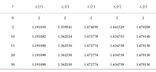
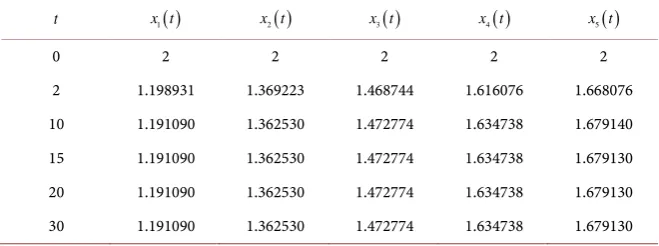
The numerical solution of the proposed optimization problem (13) can be obtained by pursuing the procedure stated in the previous example and solving the resulting nonlinear system of ODEs. The obtained numerical results from the proposed methods are presented in Tables 1-3. In Table 1 and Table 2, we presented the numerical solution x t

( )

=

(

x t1

( ) ( )

,x t2 ,,x t5

( )

)

using the GEM and the RK4 method at ν =1, respectively. But in Table 3, we presented the

numerical solution of the same system (15) using the proposed method with

0.9

[image:6.595.210.538.574.727.2]

ν = . From these tables, we can conclude that our solutions of the proposed method are in excellent agreement with the RK4 method. In addition, we can see that the behavior of the solution is in agreement with the physical meaning of the proposed problem.

Table 1. The numerical solution of Example 2 using GEM at ν=1.

t x t1( ) x t2( ) x t3( ) x t4( ) x t5( )

0 2 2 2 2 2

2 1.191010 1.359541 1.474039 1.641529 1.679209

10 1.191082 1.362524 1.472778 1.634755 1.679140

15 1.191090 1.362530 1.472774 1.634738 1.679130

20 1.191090 1.362530 1.472774 1.634738 1.679130

[image:7.595.209.539.90.213.2]

DOI: 10.4236/am.2017.812126 1767 Applied Mathematics Table 2. The numerical solution of Example 2 using the RK4 method at ν =1.

t x t1( ) x t2( ) x t3( ) x t4( ) x t5( )

0 2 2 2 2 2

2 1.191010 1.359541 1.474039 1.641529 1.679209

10 1.191082 1.362524 1.472778 1.634755 1.679140

15 1.191090 1.362530 1.472774 1.634738 1.679130

20 1.191090 1.362530 1.472774 1.634738 1.679130

30 1.191090 1.362530 1.472774 1.634738 1.679130

Table 3. The numerical solution of Example 2 using GEM at ν =0.9.

t x t1( ) x t2( ) x t3( ) x t4( ) x t5( )

0 2 2 2 2 2

2 1.198931 1.369223 1.468744 1.616076 1.668076

10 1.191090 1.362530 1.472774 1.634738 1.679140

15 1.191090 1.362530 1.472774 1.634738 1.679130

20 1.191090 1.362530 1.472774 1.634738 1.679130

30 1.191090 1.362530 1.472774 1.634738 1.679130

5. Conclusion

We implemented the GEM for studying the numerical solution for the system of FDEs which described the NLP model. This work is devoted to introduce a study of the behavior of the numerical solution of the proposed problem for various fractional Brownian motions and also for standard motion ν =1. Also, we

compared the obtained numerical solutions with those numerical solutions using RK4 method. From this study, we can see that the obtained numerical solution using the suggested method is in excellent agreement with the numerical solution using RK4 method and shows that this approach can be solved the problem effectively and illustrates the validity and the great potential of the proposed technique. Finally, the recent appearance of FDEs as models in some fields of applied mathematics makes it necessary to investigate analytical and numerical methods for such equations.

Acknowledgements

We thank the Editor and the Referees for their comments.

References

[1] Podlubny, I. (1999) Fractional Differential Equations. Academic Press, New York. [2] Khader, M.M. and Adel, M. (2016) Numerical Solutions of Fractional Wave

[image:7.595.209.539.247.370.2]

DOI: 10.4236/am.2017.812126 1768 Applied Mathematics Solving Fractional Integro-Differential Equations. ANZIAM, 51, 464-475. https://doi.org/10.1017/S1446181110000830

[4] Khader, M.M. (2011) On the Numerical Solutions for the Fractional Diffusion Equ-ation. Communications in Nonlinear Science and Numerical Simulations, 16, 2535-2542. https://doi.org/10.1016/j.cnsns.2010.09.007

[5] Oldham, K.B. and Spanier, J. (1974) The Fractional Calculus. Academic Press, New York.

[6] Luenberger, D.G. (1973) Introduction to Linear and Nonlinear Programming. Ad-dison-Wesley, Boston.

[7] Özdemir, N. and Evirgen, F. (2010) A Dynamic System Approach to Quadratic Programming Problems with Penalty Method. Bulletin of the Malaysian Mathemat-ical Sciences Society, 10, 79-91.

[8] K.J. Arrow, Hurwicz L. and Uzawa, H. (1958) Studies in Linear and Non-Linear Programming. Stanford University Press, Redwood City.

[9] Yamashita, H. (1976) Differential Equation Approach to Nonlinear Programming. Mathematical Programming, 1, 155-168.

[10] Sun, W. and Yuan, Y. (2006) Optimization Theory and Methods: Nonlinear Pro-gramming. Springer-Verlag, New York.

[11] Fiacco, A.V. and Mccormick, G.P. (1968) Nonlinear Programming: Sequential Un-constrained Minimization Techniques. John Wiley, New York.

[12] Odibat, Z.M. and Shawagfeh, N.T. (2007) Generalized Taylor’s Formula. Applied Mathematics and Computation, 186, 286-293.

https://doi.org/10.1016/j.amc.2006.07.102

[13] Arafa, A.A.M., Rida, S.Z. and Khalil, M. (2012) Fractional Modeling Dynamics of HIV and CD4+ _{T-Cells during Primary Infection. Nonlinear Biomedical Physics, 6,}

1-7. https://doi.org/10.1186/1753-4631-6-1

[14] Schittkowski, K. (1987) More Test Examples for Nonlinear Programming Codes. Springer-Verlag, Berlin.