Mapping Quantitative Trait Loci by Controlling Polygenic Background Effects

INVESTIGATION

Mapping Quantitative Trait Loci by Controlling

Polygenic Background Effects

Shizhong Xu1 Department of Botany and Plant Sciences, University of California, Riverside, California 92521

ABSTRACTA new mixed-model method was developed for mapping quantitative trait loci (QTL) by incorporating multiple polygenic covariance structures. First, we used genome-wide markers to calculate six different kinship matrices. We then partitioned the total genetic variance into six variance components, one corresponding to each kinship matrix, including the additive, dominance, additive3additive, dominance3dominance, additive3dominance, and dominance3additive variances. The six different kinship matrices along with the six estimated polygenic variances were used to control the genetic background of a QTL mapping model. Simulation studies showed that incorporating epistatic polygenic covariance structure can improve QTL mapping resolution. The method was applied to yield component traits of rice. We analyzed four traits (yield, tiller number, grain number, and grain weight) using 278 immortal F2 crosses (crosses between recombinant inbred lines) and 1619 markers. We found that the relative importance of each type of genetic variance varies across different traits. The total genetic variance of yield is contributed by additive3 additive (18%), dominance3dominance (14%), additive3dominance (48%), and dominance3additive (15%) variances. Tiller number is contributed by additive (17%), additive 3 additive (22%), and dominance 3 additive (43%) variances. Grain number is mainly contributed by additive (42%), additive 3 additive (19%), and additive 3 dominance (31%) variances. Grain weight is almost exclusively contributed by the additive (73%) variance plus a small contribution from the additive3additive (10%) variance. Using the estimated genetic variance components to capture the polygenic covariance structure, we detected 39 effects for yield, 39 effects for tiller number, 24 for grain number, and 15 for grain weight. The new method can be directly applied to polygenic-effect-adjusted genome-wide association studies (GWAS) in human and other species.

E

PISTATIC effects refer to interactions of allelic effects between different loci. Depending on the natures of pop-ulations, the variance of epistatic effects for a quantitative trait may be partitioned into several different types of variance components, e.g., additive3 additive, additive3 dominance, dominance3additive, and dominance3 dom-inance (Cockerham 1954). The relative importance of each variance component usually varies across different traits. Accurate partitioning of these epistatic variance components can help understand the genetic mechanisms of complex traits and develop more efficient breeding programs. Prior to the genome era, special designs of experiments were re-quired to partition the epistatic variance into different var-iance components, e.g., the NC design III (Cockerham and

Zeng 1996). The well-known Cockerham’s epistatic model (Cockerham 1954) is the principle basis for data analysis. With molecular data, marker genotypes can be observed and thus complicated designs are no longer crucial. For ex-ample, the recombinant inbred line (RIL) design allows us to estimate the additive3additive effects between pairs of markers. The F2 design facilitates estimation of all the four types of epistatic effects. These simple designs of experi-ments are very popular in crops and laboratory animals.

Quantitative trait locus (QTL) mapping for epistatic ef-fects has attracted much attention from geneticists (Cockerham and Zeng 1996; Kao and Zeng 2002; Yi and Xu 2002; Xu 2007; Xu and Jia 2007; Garciaet al.2008). The main hurdle in epistatic effect QTL mapping is the large number of in-teraction effects to estimate. For low-density marker maps, all pairwise interactions can befit simultaneously into a sin-gle model (Yi and Xu 2002; Xu 2007). With high-density marker maps, simultaneousfit of all genetic effects to a sin-gle model is prohibited. Anad hocmethod is tofit one pair of loci at a time and the entire genome is then scanned in Copyright © 2013 by the Genetics Society of America

doi: 10.1534/genetics.113.157032

Manuscript received July 7, 2013; accepted for publication September 16, 2013; published Early Online September 27, 2013.

Supporting information is available online athttp://www.genetics.org/lookup/suppl/ doi:10.1534/genetics.113.157032/-/DC1

a two-dimensional approach (Bell et al. 2011). It is well known in genome-wide association studies (GWAS) that such a genome-wide scanning has ignored the polygenic effect and thus will inflate the residual error variance (Yu et al.2006; Zhanget al.2010; Zhou and Stephens 2012). As a consequence, the statistical power may be low. When the pedigree relationship of individuals is known, one can fit a polygenic effect to the model using the standard linear mixed-model approach (Henderson 1975), as done for the inbred lines of maize (Zhang et al. 2005). However, the pedigree relationship is rarely known in a randomly sampled population. Yuet al.(2006) proposed using marker-inferred kinship matrix to capture the polygenic variance. This ap-proach has now become the standard method for GWAS. Efficient algorithms have been proposed afterward to im-prove the computational efficiency (Kanget al.2008; Zhang et al.2010; Lippertet al.2011; Zhou and Stephens 2012). However, such a polygenic mixed linear model has not been investigated in GWAS for epistatic effects.

QTL mapping (genome-wide linkage studies) is slightly different from GWAS because the target populations for the two approaches of genetic mapping are often different. However, if analyses are focused on markers only (ignoring pseudo-markers between observed markers), the statistical methods are much the same for the two approaches except that the random population GWAS requires an extra term in the model to control for population structures. The linear mixed-model GWAS incorporating marker-inferred kinship matrix as the covariance structure can be naturally adopted here for QTL mapping to capture the background genetic information. For a well-controlled mapping population,e.g., the F2 population, the marker inferred kinship matrix is equivalent to the identical-by-descent (IBD) matrix of poly-genes. Using this matrix to model the covariance structure plays a similar role to the cofactors added to the interval mapping, the so-called composite interval mapping as pro-posed by Jansen (1994) and Zeng (1994). A more appealing feature of this kinship-corrected QTL mapping approach is that it is easy to control the genetic background information caused by epistatic effects. The original composite interval mapping, in principle, can take into account pairwise inter-action terms as cofactors, but no attempt has been made because of the difficulty of choosing the pairwise cofactors. If the covariance structure includes kinship matrices for var-ious epistatic effects, the genetic background due to epistatic effects can be controlled.

Motivated by the above arguments, we propose a mixed-model GWAS for epistatsis using ultra-high-density SNP markers. Xie et al. (2010) and Yu et al. (2011) released a high-density SNP map containing about 270,000 SNPs. From the SNPs, they inferred recombination breakpoints for 240 RILs of a rice population derived from two inbred lines. The authors further combined consecutive SNP markers of cosegregation into bins. Within a bin, there are no breakpoints and thus all SNPs within the same bin have exactly the same genotypes. The.270,000 SNPs were

even-tually converted into 1619 bins. Each bin was then treated as a synthetic marker. Genetic analysis was then performed on the bin genotypes. Using the binned genotypes, Yuet al. (2011) conducted QTL mapping for seven yield component traits in rice and identified numerous QTL. Using the 240 RILs, Hua et al.(2002) and Huaet al.(2003) created 360 crosses to dissect epistatic effects and to investigate the ge-netic basis of heterosis for yield component traits. Most re-cently, Zhouet al.(2012) reinvestigated the genetic basis of heterosis using 278 of the 360 crosses. They called the RIL-generated crosses immortal F2 (IMF2) because the geno-types of the crosses mimic the genogeno-types of the regular F2 population. The IMF2 crosses are also called recombinant inbred intercrosses (RIX) in laboratory mice derived from crosses of multiple RILs (Zou et al. 2005). Zhou et al. (2012) used the 1619 bins as synthetic markers to test all pairwise interaction effects using a two-dimensional scan-ning approach by fitting one pair of bins at a time. The purpose of their study was to evaluate the relative impor-tance of dominance and epistasis to heterosis.

In this study, we analyzed the same IMF2 population using genotypes of the 1619 bins. We first evaluated the relative importance of each type of epistatic effects on four yield component traits using variance component analysis and then mapped epistatic effects using marker-generated kinship matrices to control the epistatic genetic background.

Material and Methods

Plant materials and SNP bin map

1998 and 1999). The phenotypic values of the two replicates were pooled for each cross after removing the year effects using

yj¼

1 2

h

yj12y1

þyj22y2

i

; (1)

wherey1andy2are the mean values of the trait measured in

1998 and 1999, respectively. This pooled trait value was treated as the actual phenotypic value for analysis. Appar-ently, we ignored the genotype by year interaction (G3E) effects, if there is any.

Polygenic variance component analysis

We first numerically coded the genotype of individual jat binkinto two variables,

Zjk¼

8 < : þ1 0 21 for for for A H

B;  Wjk¼

8 < : 0 1 0 for for for A H B; (2)

where Zjk and Wjk represent the codes for additive and dominance effects, respectively. Let y be an n31¼ 27831 column vector for the phenotypic values of all the IMF2 crosses. The full epistatic model form¼1619 bins is described by

y¼XbþP

m

k¼1

ZkakþP m

k¼1

Wkdkþ P m21

k¼1

Pm k9¼kþ1ð

Zk#Zk9ÞðaaÞ_kk9

þmX21

k¼1

Xm

k9¼kþ1

ðWk#Wk’ÞðddÞkk’þ X m21

k¼1

Xm

k9¼kþ1

ðZk#Wk9ÞðadÞkk9

þX

m21

k¼1

Xm

k9¼kþ1

ðWk#Zk9ÞðdaÞkk9þe; (3)

whereXbrepresents some nongenetic effects,e.g., intercept in this case, andeNð0;Is2_{Þ is a vector of residual errors}

with a normal distribution of unknown variance s2_{. In}

ad-dition, Zk#Wk represents element-wise vector multiplica-tion, andakanddkare the additive and dominance effects, respectively, for bink. The four terms,ðaaÞkk’,ðddÞkk9,ðadÞkk9

andðdaÞ_kk9are the additive3additive, dominance3 dom-inance, additive 3 dominance and dominance 3 additive effects, respectively, between binskandk9. These four terms are called the epistatic effects. The total number of genetic effects in the above model is

2mþ4mðm21Þ=2¼2m2¼2316192¼ 5;242;322; (4)

which is beyond the capability of any models currently available in genome-wide association studies in a simul-taneous manner. By treating each genetic effect as a ran-domly distributed normal variable with mean zero and a common variance across all bins or pairs of bins, the model becomes a mixed model. Let akNð0;s2aÞ, dk

Nð0;s2_dÞ,ðaaÞkk9Nð0;s2aaÞ, ðddÞkk9Nð0;s2ddÞ, ðadÞkk9 Nð0;s2_adÞ;and ðdaÞkk9Nð0;s2daÞ be the distributions. The fact that the variance of each type of genetic effects does not depend on the bins or bin pairs implies that all effects of the same kind share a common genetic variance. These common variances are called polygenic variances. The ex-pectation of y is EðyÞ ¼Xb and the variance–covariance matrix ofyis

varðyÞ ¼Kas2aþKds2dþKaas2aaþKdds2ddþKads2ad

þKdas2daþIs2; (5)

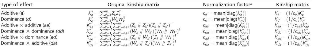
where the K’s are marker-generated kinship matrices; i.e., they depend onZkandWk. Formulas to calculate these kinship matrices are given in Table 1. Note that the kinship matrices for epistatic variances presented here are dif-ferent from the one given by Oberet al.(2012), who used the Hadamard square of the additive kinship matrix as the additive 3 additive kinship matrix. They did not detect any epistatic variance in their Drosophila melanogaster population, likely due to the use of wrong additive 3 additive kinship matrix. Given these marker-generated kinship matrices, the variance components were estimated using standard mixed-model procedures (Henderson 1975).

One may rewrite the variance–covariance matrix in Equa-tion 5 by

varðyÞ ¼ ðKalaþKdldþKaalaaþKddlddþKadlad

þKdaldaþIÞs2; (6)

where la¼s2a=s2 is the ratio of the additive genetic vari-ance to the residual varivari-ance and otherl’s are defined sim-ilarly. A more useful measurement of the relative importance of a type of genetic effect,e.g., the additive effect, is Table 1 Formulas used to calculate marker generated kinship matrices

Type of effect Original kinship matrix Normalization factora _{Kinship matrix}

Additive (a) K*

a ¼Pmk¼1ZkZkT ca¼mean½diagðKa*Þ Ka¼ ð1=caÞKa*

Dominance (d) K*

d¼

Pm

k¼1WkWkT cd¼mean½diagðKd*Þ Kd¼ ð1=cdÞK*d

Additive3additive (aa) K*

aa¼Pmk¼211

Pm

k’¼kþ1ðZk#Zk’ÞðZk#Zk’ÞT caa¼mean½diagðKaa*Þ Kaa¼ ð1=caaÞKaa*

Dominance3dominance (dd) K*

dd¼

Pm21

k¼1

Pm

k’¼kþ1ðWk#Wk’ÞðWk#Wk’ÞT cdd¼mean½diagðKdd* Þ Kdd¼ ð1=cddÞKdd*

Additive3dominance (ad) K*

ad¼

Pm21

k¼1

Pm

k’¼kþ1ðZk#Wk’ÞðZk#Wk’ÞT cad¼mean½diagðKad*Þ Kad¼ ð1=cadÞKad*

Dominance3additive (da) K*

da¼

Pm21

k¼1

Pm

k’¼kþ1ðWk#Zk’ÞðWk#Zk’ÞT cda¼mean½diagðKda*Þ Kda¼ ð1=cdaÞKda*

h2_a¼s 2 a s2 P

¼ s2a

s2

aþs2dþs2aaþsdd2 þs2adþs2daþs2 ; (7)

where the denominator (the sum of all variance compo-nents) is called the phenotypic variance. The above ratio is called the narrow-sense heritability. The broad-sense heri-tability is define by

H¼ s

2

aþs2dþs2aaþs2ddþs2adþs2da s2

aþs2dþs2aaþsdd2 þs2adþs2daþs2

: (8)

Note that the broad-sense heritability using marker-generated kinship is often close to unity when the marker density is sufficiently high. Therefore, it is not an informative piece of information. However, the proportion of each variance component relative to the total phenotypic variance is informative and is the focus of discussion in this study.

Model for genome scanning

Individual bin effects and bin pair interaction (epistatic) effects can be estimated after fitting the polygenic effects. The idea of the mixed-model GWAS (Yuet al.2006) can be adopted here. The polygenic term remains in the model except that we used six kinship matrices to describe the co-variance structure. The genetic effects of each bin and the epistatic effects of each pair of bins are modeled like the usual GWAS (Yu et al.2006) with the polygenic structure included. The epistatic model appears like

y¼Xbþjþe

þZkakþWkdkþZk9ak9þWkdk9þ ðZk#Zk9ÞðaaÞkk9 þðWk#Wk9ÞðddÞkk9þ ðZk#Wk9ÞðadÞkk9

þðWk#Zk9ÞðdaÞkk9

(9)

for locikandk9, wherejis the polygenic effect (the sum of all genetic effects across the entire genome). There are two addi-tive effects, two dominance effects, and four epistatic effects (denoted by double symbols with double subscripts) for each pair of bins. A complete scan under the epistatic model requires a two-dimensional search for all pairs of bins. We noted that the additive and dominance effects would be estimated multi-ple times. The inclusion of polygenic effects allows us to search for bin effects and epistatic effects separately. The model that includes the additive and dominance effects is

y¼XbþZkakþWkdkþjþe: (10)

A complete scan for this model (10) requiresmcalls of the above model and two genetic effects are estimated under each call. The epistatic effect model excluding the additive and dominance effects is

y¼Xbþjþeþ ðZk#Zk9ÞðaaÞkk9þ ðWk#Wk9ÞðddÞkk9

þðZk#Wk9ÞðadÞkk9þ ðWk#Zk9ÞðdaÞkk9: (11)

A complete scan for this model (11) requires mðm21Þ=2 calls of the above model and four epistatic effects are esti-mated under each call. The mixed model can be written generically as

y¼XbþZgþe; (12)

wheree¼jþeis a general error term withEðeÞ ¼0 and

varðeÞ ¼varðjÞ þIs2¼ ðKþIÞs2: (13)

Matrix K is a weighted sum of all effect-specific kinship matrices, it is not the kinship matrix given by Yu et al. (2006) in the original GWAS study,

K¼KalaþKdldþKaalaaþKddlddþKadladþKdalda;

(14)

and the weights are the ratios of the variance components to the residual variance. For the additive and dominance effect model, Z¼ZkjjWk and g¼ ½ak dkT. For the epistatic ef-fect model,

Z¼ ðZk#Zk9ÞjjðWk#Wk9ÞjjðZk#Wk9ÞjjðWk#Zk9Þ

g¼ ½ ðaaÞ_kk9ðddÞ_kk9ðadÞ_kk9ðdaÞ_kk9T;

(15)

where the special notation a||b indicates column concate-nation of matrices a andb. The vector of genetic effects g has been treated asfixed effects in the classical GWAS (Yu et al.2006; Zhou and Stephens 2012). In this study, we treat g as random effects with a multivariate Nð0;Is2

gÞ distribu-tion. The shared common variances2

g is estimated from the data. Whens2_gis set toN, the genetic effectsgbecomefixed effects.

A two-step approach to genome scanning

Polygenic analysis: The mixed-model analysis would in-clude seven genetic variance components (six polygenic variances and one genetic variance for each bin or bin pair). The six polygenic variances change very little across bins or bin pairs. Therefore, we adopted the two-step approach for parameter estimation to save computational time (Zhang et al. 2010; Lippert et al. 2011). In thefirst step, we esti-mated only the polygenic variances using the model

y¼Xbþjþe; (16)

where

varðyÞ ¼varðjÞ þvarðeÞ ¼ ðKþIÞs2: (17)

Genome scanning: We proposed the following eigen de-composition algorithm that does not require repeated in-verse of matrix KþI. Eigen decomposition for GWAS was originally proposed by Lippert et al. (2011) and later ex-tended by Zhou and Stephens (2012). The eigen decompo-sition for the kinship matrix is K¼UDUT_{, where U is the}

eigenvector (ann3nmatrix) andD¼diagðd1; :::;dnÞis the eigenvalue (a diagonal matrix). One property of the eigen decomposition isK21_¼UD21_UT_{, which has avoided matrix}

inversion because D21 _{is simply the inverse of a diagonal}

matrix. The error variance is rewritten by

varðeÞ ¼varðjþeÞ ¼ ðKþIÞs2¼ ðUDUTþIÞs2

¼UðDþIÞUTs2: (18)

Before calling the mixed-model procedure, we performed data transformations so that the mixed model is rewritten by

UTy¼UTðXbþZgþeÞ ¼UTXbþUTZgþUTe: (19)

Let y*¼UT_{y be the transformed phenotypic values. The}

model for the transformed data is

y*¼X*bþZ*gþe*: (20)

The expectation and variance matrix of the transformed data areEðy*Þ ¼X*band

varðe*Þ ¼varðUTeÞ ¼UTðKþIÞUs2¼UTðUDUTþIÞUs2

¼ ðDþIÞs2;

(21)

respectively. Let

W¼ ðDþIÞ21¼diag h

ðd1þ1Þ21; :::;ðdnþ1Þ21

i (22)

be a weight matrix. The residual variance structure for the transformed data are

varðe*Þ ¼R¼W21s2: (23)

The mixed-model equations for BLUE ofband BLUP ofgare

X*T_{WX* X}*T_WZ* Z*T_{WX* Z}*T_WZ*þI=_s2

g b g ¼

X*T_Wy* Z*T_Wy*

: (24)

The null hypothesis may be tested in one of two ways. One way is the likelihood ratio test under the null model H0:s2g ¼0. The other way is the Wald test under the null modelH0:g¼0. The mixed-model equations provide both

the BLUP of g and the variance–covariance matrix of the BLUP estimate. The Wald test statistic is

Wald¼g^T½varðg^Þ21g^: (25)

When g¼0 is true, the Wald test statistic follows a chi-square distribution with 2 degrees of freedom for the

additive-dominance model and 4 degrees of freedom for the epistatic effect model.

Software implementation

All data analyses were implemented using the restricted maximum-likelihood (REML) method (Patterson and Thompson 1971) implemented via the MIXED and HPMIXED proce-dures in SAS (SAS Institute 2009b). PROC IML (SAS In-stitute 2009a) was also used to calculate eigenvalues and eigenvectors and to perform data transformations. The poly-genic variance component analysis was conducted using PROC MIXED. Genome scans were implemented using PROC HPMIXED, which is a specialized high-performance version of the MIXED procedure. The SAS codes are provided in Supporting Information,File S11for PROC MIXED andFile S12for PROC HPMIXED. The six types of kinship matrices are given in File S1. The phenotypes of four quantitative traits are given in File S2. Genotypes of two bins (bins 729 and 1064) are given inFile S3.

Results

Results of a simulation experiment

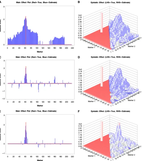
Before analyzing the rice data, we wanted to show the difference of genomic scans between the model including the polygenic variances and the model without the poly-genic variances using simulated data. Similar comparison has been performed in the traditional mixed-model GWAS that ignored the epistatic polygenic variance (Yu et al. 2006). We used the genotypes of 217 bins on thefirst chro-mosome for the 278 IMF2 crosses of rice as the simulated genotypes and added some effects on bins and bin pairs to generate genetic values of all crosses. We then added a nor-mally distributed residual error to the genetic value of each cross to form a phenotypic value for the cross. To simplify the model, we simulated only the additive effects and the additive3additive effects. For 217 bins, the model in-cluded 217 additive effects and 217ð21721Þ=2¼23437 additive 3additive effects. Therefore, the polygenic model contained two genetic variance components.

sharper than the previous two models. For the simple ex-periment, the model ignoring polygenic covariance struc-ture already performed well.

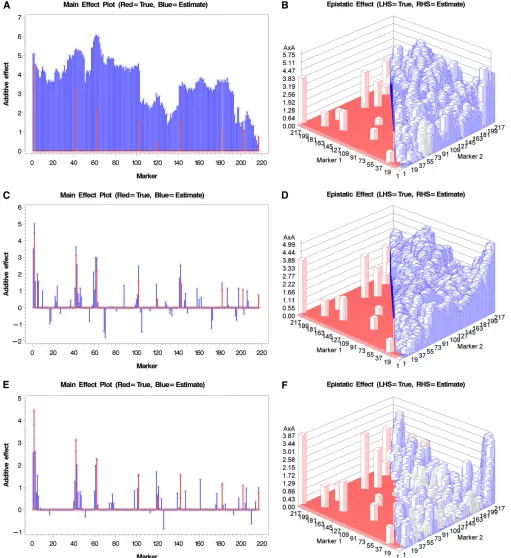
Figure 2, red and blue, respectively. The improvement of the models including the polygenic effects over the model ignor-ing them is more obvious in the complicated experiment. For the model ignoring the polygenic covariance structure (Fig-ure 2, A and B), peaks of the estimated main effects do not correspond to the true values at all. The estimated epistatic effects correspond to the true effects when the true effects are large. When the additive covariance structure is incor-porated in the model, improvement for the main effects is obvious (Figure 2C) but the epistatic effects have very little improvement (Figure 2D). Figure 2, E and F, show the main and epistatic effects, respectively, for the model incorporated both the additive and additive3additive covariance struc-tures. The improvement is much clearer compared with the previous two models. The simulation experiments by no means were exhausted but they provided visual evidence that the polygenic-effect-adjusted model performed better than the model without the polygenic effects. Incorporating epistatic covariance structure led to further improvement.

Polygenic variance analysis for yield component traits in rice

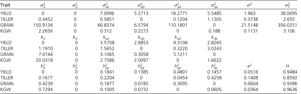
Results of the variance component analyses are summarized in Table 2. The variance ratios (lX¼s2X=s2) are also listed in the table and they were used to calculate the weighted sum of different kinship matrices. The most important in-formation from the table is the proportion of the phenotypic variance contributed by each type of genetic variance (h2

X¼s2X=s2P). Several general conclusions were drawn from

the observations: (1) None of the four traits were contrib-uted by the dominance variance; (2) the additive variances contributed the most in two of the four traits (GRAIN and KGW); (3) the additive3dominance variance is important for YIELD and dominance 3additive variance is important for TILLER; (4) the KGW trait was almost exclusively con-trolled by the additive variance; and (5) all the four traits had high broad sense heritability with KGW being the high-est (H¼0:9636). The goodness offit (squared correlation between predicted and observed phenotypic values) was almost perfect for all traits. The likelihood ratio test (LRT) statistics for the polygenic effect model (including all six genetic variance components) were all high (37.9, 58.2, 82.2, and 248.9) with extremely smallP-values (1.17E–06, 1.04E–10, 1.25E–15, and 7.04E–51) for the four traits. The significant polygenic variance for each of the four traits im-plied that polygenic-effect-adjusted model should perform better than the model ignoring the polygenic effects. Note that the goodness offit is not exactly the same as the broad sense heritability because the two are calculated using dif-ferent formulas, in which varðyÞ was calculated from the data and s2P was calculated from the sum of all variance

components. The polygenic analysis provides only a general picture of the relative importance of each type of variance components. When a variance component is zero, it means that this type of effect is not as important as some other types of effects in general. It does not exclude the possibility

that some bins may have significant effects of this type, which have been “diluted” in the polygenic analysis (see more discussion in the last section).File S11gives the SAS code of PROC MIXED for the polygenic analysis.

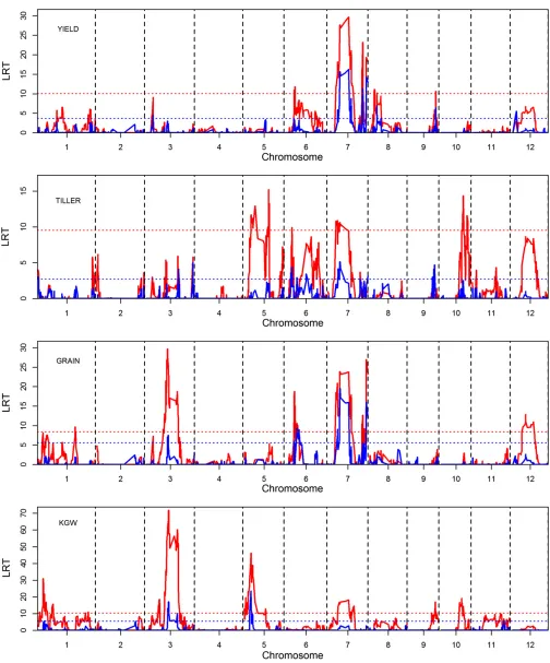
Genome scans for yield component traits in rice

Main effect analysis:We used two models to perform the main effect analysis. One model contains the additive and dominance effects of each bin plus the polygenic effect captured by the polygenic covariance structure (all six types of polygenic variances were considered). The method is called weighted mixed-model analysis. The second model contains the additive and dominance effects for each bin but ignores the polygenic covariance structure. This method is called unweighted mixed-model analysis. The comparison provides a real life demonstration of the differences between the two models. The LRT statistic was used to declare statistical significance for each bin. The critical values for the LRT test statistics were determined via multiple permuta-tions to adjust for multiple tests (Churchill and Doerge 1994). The polygenic covariance structures were reserved. The number of reshuffled samples in the permutation tests was 1000 per trait within each method. The maximum LRT was recorded for each permuted sample. For a total of 1000 permuted samples, we obtained 1000 such maximum LRT values. These maximum LRT values form an empirical null distribution. The LRT value of each bin from the original data analysis (not from the reshuffled data) was then com-pared to the null distribution. TheP-value is the proportion of the 1000 permuted samples whose LRT values are greater than the LRT of the original data analysis. First, let us eval-uate the critical values of the test statistics from the null distributions. The 90, 95, 99, and 100 percentiles of the null distributions are listed in Table 3 (the top and middle por-tions of the table). The critical values for the unweighted method are always higher than the weighted method. For example, the critical value for YIELD at type I error of 0.05 is 3.6711 for the weighted method, but the corresponding value for the unweighted method is 10.0605. The critical values also vary across different traits, indicating that per-mutation tests are necessary.

due to linkage disequilibrium. For example, about 50 bins covering one-third of chromosome 3 for trait GRAIN are significant for the unweighted method due to high linkage

along with theP-values of the 1619 bins for all the four traits are provided in File S4 and File S5 for the weighted and unweighted methods, respectively.

We now focus only on the weighted mixed-model analysis and report all bins that passed a preliminary screen to eliminate all bins with LRT less than 4.61, equivalent to LOD score less than one. All bins withP-values,0.05 were declared as significant at the genome-wide type I error of 0.05. Using theP-value ,0.05 criterion, the number of sig-nificant bins are 25, 4, 32, and 23 for traits YIELD, TILLER, GRAIN, and KGW, respectively. These numbers are not the numbers of detected QTL because consecutive bins tended to show cosegregation. Therefore, the actual numbers of QTL are less than the number of significant bins. For exam-ple, among the four significant bins (bins 534, 1004, 1005, and 1262) for trait TILLER, only three QTL can be declared because bins 1004 and 1005 are counted as one due to their high linkage.File S6 lists all the bins passing the preselec-tion, including the significant bins drawn from the permu-tation tests for the four traits. The estimated numbers of QTL are presented later using another round of screening to remove redundant bins caused by close linkage.

Epistatic effect analysis: Due to limitation of computing power, we used only the polygenic-effect-adjusted model (weighted method) to analyze the yield component traits. The LRT statistic was used to declare statistical significance for bin 3 bin interactions. The critical value for the LRT statistics was determined via a permutation analysis (Churchill and Doerge 1994) to adjust for multiple tests. For the epistatic effect model, we first eliminated all bin pairs with LRT,9.22, equivalent to LOD score,2. We then used the survived bin pairs to perform permutation analysis. The maximum LRT test statistics of 1000 permuted samples form an empirical null distribution. The 90, 95, 99, and 100 percentiles of the permutation-drawn null distributions for the four traits are given in Table 3 (bottom). These critical values also vary across traits. Trait KGW had the highest

critical values and trait TILLER had the lowest critical val-ues. The percentiles for the epistatic effect model are sub-stantially higher than the percentiles for the main effect model. For example, the LRT critical value of KGW at 0.05 type I error is 5.47 for the main effect model but it is 15.77 for the epistatic effect model. TheP-values were drawn for each pair of bins and the significant bin pairs along with their estimated effects are listed in File S7. The numbers of significant bin pairs are 1071, 205, 573, and 66 for traits YIELD, TILLER, GRAIN, and KGW, respectively. Again, these numbers are not the estimated numbers of epistatic effects due to tight linkage of consecutive bins. The estimated num-ber of QTL interactions is addressed below using another cycle of screening.

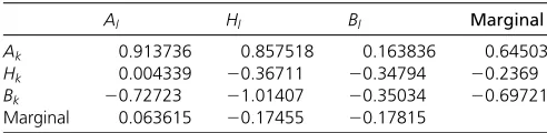
For trait KGW in the epistatic effect model analysis, bin pairðk;lÞ ¼ ð729;1064Þhad an LRT of 18.23049 with aP -value of 0.016. We now provide a detailed analysis for this pair of bins. We used a model that includes the additive and dominance effects for both bins and all the four epistatic effects. The six polygenic covariance structures were also included in the model. This revised model now contains eight genetic effects and an intercept. Reanalysis of this bin pair produced eight estimated genetic effects, which are further converted into nine genotypic values using the transformation 2 6 6 6 6 6 6 6 6 6 6 6 6 4

0:913736 0:857518 0:163836 0:004339

20:36711

20:34794

20:72723

21:01407

20:35034

3 7 7 7 7 7 7 7 7 7 7 7 7 5 ¼ 2 6 6 6 6 6 6 6 6 6 6 6 6 4

1 1 0 0 1 0 0 0 1 0 0 1 0 1 0 0 1 21 0 0 21 0 0 0 0 1 1 0 0 0 1 0 0 0 1 1 0 0 0 1 0 21 1 0 0 0 21 0

21 1 0 0 21 0 0 0

21 0 0 1 0 21 0 0

21 21 0 0 1 0 0 0

3 7 7 7 7 7 7 7 7 7 7 7 7 5 2 6 6 6 6 6 6 6 6 6 6 4

0:538786 0:093253

20:1718

20:07827 0:281697 0:397007 0:082886

20:11703

3 7 7 7 7 7 7 7 7 7 7 5 ; (26)

where the vector in the right-hand side stores the esti-mated genetic effects in the following order: f^ak;^al;^dk;d^l; ðcaaÞkl;ðadcÞkl;ðcdaÞkl;ðddcÞklg. The vector in the left-hand side Table 2 Estimated variance components and proportions of variances over the phenotypic variance

Trait s2

a s2d s2aa s2dd s2ad s2da s2 s2P

YIELD 0 0 7.0096 5.2713 18.2771 5.5485 1.963 38.0695

TILLER 0.4452 0 0.5851 0 0.1204 1.1305 0.3738 2.655

GRAIN 150.9134 0 66.8374 6.5794 110.1801 0 21.5148 356.0251

KGW 2.2656 0 0.312 0.2273 0 0.188 0.1131 3.106

l_a l_d l_aa l_dd l_ad l_da

YIELD 0 0 3.5708 2.6853 9.3108 2.8265

TILLER 1.1910 0 1.5652 0 0.3220 3.0243

GRAIN 7.0144 0 3.1065 0.3058 5.1211 0

KGW 20.0318 0 2.7586 2.0097 0 1.6622

h2

a h2d h2aa hdd2 h2ad h2da e2 H

YIELD 0 0 0.1841 0.1385 0.4801 0.1457 0.0516 0.9484

TILLER 0.1677 0 0.2204 0 0.0454 0.4258 0.1408 0.8592

GRAIN 0.4239 0 0.1877 0.0185 0.3095 0 0.0604 0.9396

KGW 0.7294 0 0.1005 0.0732 0 0.0605 0.0364 0.9636

lX¼s2X=s2: variance ratio. h2X¼s2X=s2P: proportion of phenotypic variance contributed by each type of variance. H: the broad sense heritability defined by

H¼s2

gives the nine genotypic values. These genotypic values along with the marginal values are arranged in the following 434 matrix:

For bin l¼1064, the marginal effects are not signifi -cantly different among the three genotypes. However, the

differences are very significant under the Ak background. This detailed analysis shows the importance of the epistatic effects between the two bins for trait KGW. The two bins jointly contribute a genetic variance of 0.2991, which explains h2

kl¼0:2991=3:109210%of the total trait vari-ance. This is a significant contribution from only two loci for a quantitative trait. File S12 gives the SAS code of PROC HPMIXED for the analysis of the two bins. The genotypes of the two bins are given inFile S3.

Numbers of bins and bin3bin interactions

This step provides the last screen of the bins and bin3bin interactions that have survived all previous selections. We noted that due to close linkages between consecutive bins, multiple bins are detected in a wide range of chromosome regions. In the original study of the IMF2 population by Zhouet al.(2012), the authors set up a subjective criterion to eliminate the extra significant bins. For example, they pooled several bins in the neighborhood of a few centimor-gans of the genome into a single cluster. Each cluster was treated as one QTL. The authors realized that this approach is subjective and may eliminate some true effects. Here, we adopted a different and more objective strategy to elimi-nate those superfluous bins. Since the numbers of signifi -cant bins and bin 3 bin interactions are substantially smaller than the total number of bins and bin3bin pairs available in the data, we can fit all these significant bins

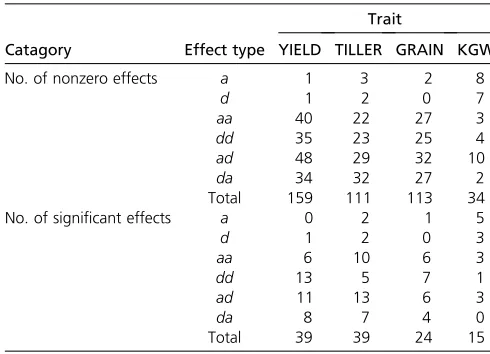
and bin pairs simultaneously in a single model. For exam-ple, there are 23 significant bins (a andd) and 66 signifi -cant bin pairs (aa, dd, ad, and da) for trait KGW, and simultaneous analysis of all 2332þ6634¼310 effects with a population size of 278 is possible, provided that a penalized regression is used to overcome the overfitting problem. For trait YIELD, the total number of significant bins and bin3bin pairs is 25 + 1071 = 1096, leading to 2532þ107134¼4334 effects, which is even harder to deal with than the KGW trait. Therefore, we used a penal-ized regression approach to perform parameter estimation, the Lasso method (Tibshirani 1996) implemented via the GlmNet/R package (Friedman et al. 2010). The method selects effects with nonzero effects (variable selection). After a minor modification of the Lasso method, the pro-gram also provides a test for each effect included in the model (Xu 2013).

The selected (nonzero) effects and their P-values obtained from the Lasso method are given in File S8 for all four traits. In this data set, if bin1 and bin2 have the same number, the effect represents a main effect; otherwise, the effect is an epistatic effect. The variable named “type” provides information about the type of effect. For example, type = “aa” indicates the additive 3 additive effect. Sig-nificant effects are labeled 1 in the last column named “significant.”The numbers of significant effects sorted by effect type for the four traits are given in Table 4, where the top shows the number of (nonzero) effects selected by the Lasso method and the bottom gives the corresponding numbers that are significant atP-value,0.05. There are 39 significant effects apiece for YIELD and TILLER. Traits GRAIN and KGW have 24 and 15 significant effects, respec-tively. The number of significant epistatic effects is often higher than the number of main effects due to the substan-tially larger number of bin3bin pairs than the number of bins. The only exception occurs for trait KGW, which has 8 significant main effects and 7 significant epistatic effects. Table 5 shows the relative contributions of different types of effects to the total phenotypic variance. The significant effects collectively contributed 0.83, 0.69, 0.68, and 0.61 of the phenotypic variances for traits YIELD, TILLER, GRAIN, and KGW, respectively. These proportions are dif-ferent from the broad sense heritability in the polygenic analysis (see Table 2). File S9 stores only the significant effects for the four traits (a subset ofFile S8).File S10gives the independent variables converted from the genotypes for all the significant effects. For example, trait KGW has 15 significant effects, and thus the data set (sheet KWG in File S10) is stored in a 153278 matrix plus the bin and effect type information.

Detailed examination of Table 5 shows that the relative contributions of different types of effects vary across traits. Epistatic effects play more important roles than main effects for traits YIELD, TILLER, and GRAIN while the additive ef-fect is more important for trait KGW. This general conclu-sion is consistent with that of the polygenic analysis. Table 3 Critical values for the LRT test statistics drawn from 1000

permuted samples

Trait

Percentile YIELD TILLER GRAIN KGW

Main (weighted) 100 9.7700 9.6460 14.5973 15.0849 99 6.3322 5.1701 8.5974 8.3822 95 3.6711 2.7129 5.5586 5.4752 90 2.9402 1.8485 4.3127 4.2637 Main (unweighted) 100 17.0252 29.8881 19.8806 18.9779 99 13.5334 12.2396 11.2226 14.8465 95 10.0605 9.5286 8.3632 10.3167 90 8.3845 8.1208 6.9026 8.4707 Epistatic 100 15.3727 21.8627 23.1942 26.2208 99 14.4295 14.1096 18.0734 18.9523 95 11.7136 11.0299 14.3440 15.7716 90 10.4775 9.1725 12.6711 14.0365

Al Hl Bl Marginal

Ak 0.913736 0.857518 0.163836 0.64503

Hk 0.004339 20.36711 20.34794 20.2369

Bk 20.72723 21.01407 20.35034 20.69721

Discussion

Epistasis is often considered important to the variation of complex traits (Cockerham 1954). However, dissection of epistasis is difficult prior to the genome era because epistatic variances are often confounded with the additive and resid-ual variances. To separate epistatic variances from additive and dominance variances, one needs pedigree information and the pedigrees must be very complicated to make the IBD matrices of epistasis sufficiently different from the kinship matrix for additive effects. In human populations, pedigree information is often incomplete and shallow (traced back to just one or two generations) and thus does not give us sufficient power to dissect epistasis. In the genome era, genome-wide marker information is available, which gives us an ample opportunity to model epistatic effects. Pedigree information is no longer crucial and a simple line cross ex-periment may be sufficient. In this study, we used binned genotypes of an IMF2 population to derive all the four types of kinship matrices to facilitate estimation of all types of epistatic variance components.

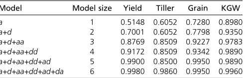
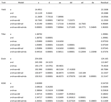
The result of the polygenic variance component analysis showed that adding epistatic variances can increase the model goodness offit. We treated the additive model as the basis and progressively added more variance components to the model in the following sequence:a,a+d,a+d+aa, a+d+aa+dd,a+d+aa+dd+ad, anda+d+aa+ dd+ad+da. Table 6 shows the increase of goodness offit expressed as the squared correlation coefficient between the observed and predicted phenotypic values for the 278 IMF2 crosses. Depending on the characteristics of different traits, the goodness of fit has increased from 51.5 to 99.8% for YIELD and from 89.8 to 99.6% for KGW. The high goodness offit implies an overfitting issue for the full model. Increas-ing sample size will partially correct the overfitting problem. Interestingly, the additive model alone alreadyfits well for all the traits, especially for trait KGW. The reason may be

explained for the high correlation between different esti-mated variance components, which may be caused by high similarities of various types of kinship matrices. The esti-mated variance components under different model sizes are listed inTable S1. Under the full model (all six genetic variance components arefit), the estimated dominance var-iances are zero for all the four traits. However, when the model size decreases, this estimated variance component can be nonzero, indicating that the actual dominance vari-ance may not be zero but it is captured by other varivari-ance components due to the high correlation. The high correla-tion of estimated genetic variance components and high similarity between different kinship matrices suggest that benefit fromfitting multiple polygenic covariance structures may not be significant for small sample sizes. Large sample sizes are necessary to separate the different genetic varian-ces. How large of a sample size is sufficiently large? Theo-retical investigation along with more simulation studies are required to have a clear answer for this question. The idea of incorporating multiple epistatic variance components in GWAS may be extended to incorporating multiple chromo-some specific variance components in GWAS. How much improvement can we get by fitting multiple chromosome variances? Again, there is no clear answer at this moment. We may need a very large sample size to show the benefit. A zero-estimated variance component for a particular type of effect does not mean that there is no genetic effect of this type for a particular bin or bin pair. The polygenic variance component of each type is the average of all bin- or bin pair-specific variances. A small number of bins or bin pairs may have large effects, but their effects are“diluted” under the polygenic model, which causes a zero estimation of the variance component. Our data analysis shows a lot of significant dominance effects but the estimated dominance variances obtained from the full model are zero for all traits. In the original study of the IMF2 population, Zhouet al. (2012) used a different model to identify epistatic effects. They fit a two-locus model using a 33 3 factorial design (two loci and three genotypes per locus) and used a two-dimensional genome scan. They did not fit the polygenic variances. How much improvement have we achieved by

fitting the polygenic variances? We do not have the answer at the moment because that would involve reanalysis of all the entire genome using the unweighted mixed model. Analysis of one trait, including permutation tests, took about 10 days of computing time because the large number of model effects fit to the model under the epistatic effect model, which is 431619ð161921Þ=2¼5;239;084, where the 4 in the expression represents the four types of epistatic effects. Advantages of fitting the polygenic variances (weighted mixed model) have been demonstrated under the main effect (a +d) model using both simulated data as well as the rice data. Our results are also not comparable with the results of Zhou et al.(2012) because we pooled data of the 2 years together and ignored the potential G3E interactions.

Table 4 Numbers of non-zero effects and numbers of significant effects (P<0.05) obtained from the Lasso analysis

Trait

Catagory Effect type YIELD TILLER GRAIN KGW

No. of nonzero effects a 1 3 2 8

d 1 2 0 7

aa 40 22 27 3 dd 35 23 25 4 ad 48 29 32 10 da 34 32 27 2 Total 159 111 113 34 No. of significant effects a 0 2 1 5

d 1 2 0 3

aa 6 10 6 3

dd 13 5 7 1

ad 11 13 6 3

da 8 7 4 0

Our study is different from the conventional GWAS (Yu et al. 2006) because we fit epistatic effects. However, the statistical model in our study shares similar properties with the improved eigenvalue decomposition methods (Lippert et al.2011; Zhou and Stephens 2012) due to thefit of poly-genic variances. We fit six variance components while the improved methods fit only one. Another difference is that we treated the bin effects and bin 3 bin interactions as random effects while Lippert et al. (2011) and Zhou and Stephens (2012) treated them as fixed effects. The advan-tages of fitting the random effects come from the shared variances and the tests of variance components. For in-stance, all the four epistatic effects share the same epistatic variance and are tested as one unit using a single LRT sta-tistics. This approach may share some of the natures in rare variant detection (Wuet al.2011), in which a group of rare variants are detected together using a single score test. Com-pared with the additive effect, an epistatic effect is a rare variant because the coefficient,e.g., Zk#Zl, has a smaller variance across individuals than the variance of Zk or Zl. Testing all four epistatic effects together will increase the statistical power for the same reason as the rare variant score test.

Finally, existing SAS programs were used here and the SAS codes are extremely simple (seeFile S11andFile S12). Theoretically, for each bin or bin pair, the six genetic vari-ance components and the bin or bin pair specific variance can be estimated simultaneously using the HPMIXED pro-cedure in SAS. This would be called the exact method (Zhou and Stephens 2012), as opposed to the approximate method (Lippert et al. 2011), where the polygenic variance is esti-mated only once before the genome is scanned. Our method is considered the approximate method because we esti-mated the polygenic variances prior to the two-dimensional scan. We did not adopt the exact method for two reasons: (1) there is a computational concern because we would have to estimate seven genetic variances per bin pair (high com-putational cost), and (2) there is no empirical evidence that

the exact method outperforms the approximate method, al-though the former is theoretically superior over the latter. Using simulated data for the main effect model, we did not see much difference between the exact and approximate methods (data not shown). Zhou and Stephens (2012) pro-posed the exact method not because the exact method is better than the approximate method, but because it will avoid any “potential risk” of the approximate method and the exact method does not increase the computing time due to a special algorithm (eigen decomposition) for likelihood function evaluation. Once the polygenic variances are trea-ted as constants in the approximate method, we provided a weight variable (see Equation 22 for the weight) to the HPMIXED procedure without modifying the code. In addi-tion, the input variables were transformed using the eigen-vector matrix prior to calling the SAS procedure. For readers without easy access to the SAS software packages, an R code is available from the author on request.

Acknowledgments

The author is grateful to two anonymous reviewers for their comments on early versions of the manuscript. The author also appreciates Dr. Qifa Zhang for sharing some additional data for the IMF2 population of rice beyond the data posted on the journal website. The project was supported by the Table 5 Genetic variances contributed by each type of genetic effects for the yield component traits in rice

Trait a d aa dd ad da Genotypea _Phenotypeb

YIELD No. effects 0 1 6 13 11 8 39

Proportion 0 0.017948 0.097888 0.144975 0.14334 0.096371 0.830223

Variance 0 0.612323 3.339706 4.946172 4.890387 3.287921 28.3251 34.117502

TILLER No. effects 2 2 10 5 13 7 39

Proportion 0.02379 0.00998 0.15154 0.04523 0.19865 0.12923 0.6855

Variance 0.05834 0.02447 0.37166 0.11092 0.4872 0.31694 1.68123 2.4525721

GRAIN No. effects 1 0 6 7 6 4 24

Proportion 0.0243 0 0.12329 0.09619 0.12649 0.09752 0.67615

Variance 6.99571 0 35.4907 27.6897 36.413 28.0731 194.643 287.87109

KGW No. effects 5 3 3 1 3 0 15

Proportion 0.35732 0.03345 0.03845 0.04702 0.087 0 0.61046

Variance 1.11098 0.10402 0.11955 0.14618 0.27049 0 1.89803 3.1091762 a_{The number of effects in this column is the sum of all the six effect-specific numbers. The variance of this column is not the sum of the six effect-specific variances because it} includes the covariance terms in addition to the effect-specific variances. The proportion of phenotypic variance contributed by genotype is also not the sum of the effect-specific proportions; rather it is the ratio of the genotypic variance to the phenotypic variance.

b_{The phenotypic variance in this column is directly calculated from the trait value, denoted by varðyÞ, and thus it is different from the phenotypic variance shown in Table 1} that is denoted bys2

P.

Table 6 Change of the goodness offita_{as the model size changes}

Model Model size Yield Tiller Grain KGW

a 1 0.5148 0.6052 0.7280 0.8980 a+d 2 0.7001 0.6052 0.7798 0.9350 a+d+aa 3 0.8769 0.8509 0.9227 0.9783 a+d+aa+dd 4 0.9172 0.8509 0.9342 0.9890 a+d+aa+dd+ad 5 0.9900 0.8500 0.9950 0.9890 a+d+aa+dd+ad+da 6 0.9980 0.9860 0.9950 0.9960 a_{The goodness offit is defined as the squared correlation coefficient between}

U.S. Department of Agriculture National Institute of Food and Agriculture Grant 2007-02784.

Literature Cited

Bell, J. T., N. J. Timpson, N. W. Rayner, E. Zeggini, T. M. Frayling et al., 2011 Genome-wide association scan allowing for epis-tasis in type 2 diabetes. Ann. Hum. Genet. 75: 10–19. Churchill, G. A., and R. W. Doerge, 1994 Empirical threshold

values for quantitative trait mapping. Genetics 138: 963–971. Cockerham, C. C., 1954 An extension of the concept of

partition-ing hereditary variance for analysis of covariances among rela-tives when epistasis is present. Genetics 39: 859–882.

Cockerham, C. C., and Z. B. Zeng, 1996 Design III with marker loci. Genetics 143: 1437–1456.

Friedman, J., T. Hastie, and R. Tibshirani, 2010 Regularization paths for generalized linear models via coordinate descent. J. Stat. Software 33: 1_–22.

Garcia, A. A., S. Wang, A. E. Melchinger, and Z. B. Zeng, 2008 Quantitative trait loci mapping and the genetic basis of heterosis in maize and rice. Genetics 180: 1707_–1724. Henderson, C. R., 1975 Best linear unbiased estimation and

pre-diction under a selection model. Biometrics 31: 423–447. Hua, J. P., Y. Z. Xing, C. G. Xu, X. L. Sun, S. B. Yu et al.,

2002 Genetic dissection of an elite rice hybrid revealed that heterozygotes are not always advantageous for performance. Genetics 162: 1885–1895.

Hua, J., Y. Xing, W. Wu, C. Xu, X. Sunet al., 2003 Single-locus heterotic effects and dominance by dominance interactions can adequately explain the genetic basis of heterosis in an elite rice hybrid. Proc. Natl. Acad. Sci. USA 100: 2574–2579.

Jansen, R. C., 1994 Controlling the type I and type II errors in mapping quantitative trait loci. Genetics 138: 871–881. Kang, H. M., N. A. Zaitlen, C. M. Wade, A. Kirby, D. Heckerman

et al., 2008 Efficient control of population structure in model organism association mapping. Genetics 178: 1709_–1723. Kao, C. H., and Z. B. Zeng, 2002 Modeling epistasis of

quantita-tive trait loci using Cockerham_’s model. Genetics 160: 1243_– 1261.

Lippert, C., J. Listgarten, Y. Liu, C. M. Kadie, R. I. Davidsonet al., 2011 FaST linear mixed models for genome-wide association studies. Nat. Methods 8: 833–835.

Ober, U., J. F. Ayroles, E. A. Stone, S. Richards, D. Zhu et al., 2012 Using whole-genome sequence data to predict quantita-tive trait phenotypes inDrosophila melanogaster. PLoS Genet. 8: e1002685.

Patterson, H. D., and R. Thompson, 1971 Recovery of inter-block information when block sizes are unequal. Biometrika 58: 545–554.

SAS Institute, 2009a SAS/IML User’s Guide,Version 9.3. SAS In-stitute Inc., Cary, NC.

SAS Institute, 2009b SAS/STAT: Users’ Guide, Version 9.3. SAS Institute Inc., Cary, NC.

Tibshirani, R., 1996 Regression shrinkage and selection via the Lasso. J. R. Stat. Soc., B 58: 267–288.

Wu, M. C., S. Lee, T. Cai, Y. Li, M. Boehnke et al., 2011 Rare-variant association testing for sequencing data with the se-quence kernel association test. Am. J. Hum. Genet. 89: 82_–93. Xie, W., Q. Feng, H. Yu, X. Huang, Q. Zhaoet al., 2010 Parent-independent genotyping for constructing an ultrahigh-density linkage map based on population sequencing. Proc. Natl. Acad. Sci. USA 107: 10578_–10583.

Xu, S., 2007 An empirical Bayes method for estimating epistatic effects of quantitative trait loci. Biometrics 63: 513–521. Xu, S., 2013 Genetic mapping and genomic selection using

re-combination breakpoint data. Genetics 195:1103–1115. Xu, S., and Z. Jia, 2007 Genomewide analysis of epistatic effects

for quantitative traits in barley. Genetics 157: 1955–1963. Yi, N., and S. Xu, 2002 Mapping quantitative trait loci with

epi-static effects. Genet. Res. 79: 185–198.

Yu, H., W. Xie, J. Wang, Y. Xing, C. Xuet al., 2011 Gains in QTL detection using an ultra-high-density SNP map based on popu-lation sequencing relative to traditional RFLP/SSR markers. PLoS One 6: e17595.

Yu, J., G. Pressoir, W. H. Briggs, I. Vroh Bi, M. Yamasaki et al., 2006 A unified mixed-model method for association mapping that accounts for multiple levels of relatedness. Nat. Genet. 38: 203–208.

Zeng, Z.-B., 1994 Precision mapping of quantitative trait loci. Ge-netics 136: 1457–1468.

Zhang, Y.-M., Y. Mao, C. Xie, H. Smith, L. Luoet al., 2005 Mapping quantitative trait loci using naturally occurring genetic variance among commercial inbred lines of maize (Zea maysL.). Genetics 169: 2267–2275.

Zhang, Z., E. Ersoz, C. Q. Lai, R. J. Todhunter, H. K. Tiwariet al., 2010 Mixed linear model approach adapted for genome-wide association studies. Nat. Genet. 42: 355–360.

Zhou, G., Y. Chen, W. Yao, C. Zhang, W. Xieet al., 2012 Genetic composition of yield heterosis in an elite rice hybrid. Proc. Natl. Acad. Sci. USA 109: 15847_–15852.

Zhou, X., and M. Stephens, 2012 Genome-wide efficient mixed-model analysis for association studies. Nat. Genet. 44: 821_–824. Zou, F., J. A. L. Gelfond, D. C. Airey, L. Lu, K. F. Manly et al., 2005 Quantitative trait locus analysis using recombinant inbred intercrosses: theoretical and empirical considerations. Genetics 170: 1299_–1311.

GENETICS

Supporting Information

http://www.genetics.org/lookup/suppl/doi:10.1534/genetics.113.157032/-/DC1

Mapping Quantitative Trait Loci by Controlling

Polygenic Background Effects

Shizhong Xu

Files S1-S10

All files are available for download at http://www.genetics.org/lookup/suppl/doi:10.1534/genetics.113.157032/-/DC1.

File S1: This dataset contains all six types of kinship matrices, each with a dimension

278 278



. The type of kinship matrix is

indicated by the first column (variable named parm) with 1, 2, 3, 4, 5, 6 indicating a, d, aa, dd, ad and da, respectively. The second column of this dataset gives the row numbers of each type of the kinship matrix. This special format is required by the PROC MIXED program. The data must contain

n



2

variables with variable names of parm, row, col1, …, coln, where n is the number of lines. Do not mess up the variable names! The type=lin(6) option in the random statement of PROC MIXED means the program is looking for 6 kinship matrices.

File S2: This dataset stores the fixed-effect-adjusted phenotypic values of the four traits, yield, tiller, grain and kgw. The first

two columns give the line id and line names. The last column gives the fold id that is used in the five-fold cross validation analysis by the Lasso method implemented via the GlmNet/R program.

File S3: This dataset gives the genotypes of two selected bins, bin1 = 729 and bin2 = 1064. The first column gives the names of

the 278 IMF2 crosses. This dataset is used by the PROC HPMIXED program shown in Script S2.

File S4: This dataset list the estimated additive (a) and dominance (d) effects for all the 1619 bins obtained from the weighted

mixed model (model incorporating the polygenic covariance structure). The standard errors corresponding to the additive and dominance effects are denoted by a_err and d_err, respectively. Effect specific tests are denoted by f_a and f_d (F test or Wald test). The LRT and p-value are also provided in the dataset. The last column gives the significant status with value 1 for p < 0.05 and 0 for p > 0.05.

File S5: This dataset list the estimated additive (a) and dominance (d) effects for all the 1619 bins obtained from the

unweighted mixed model (model ignoring the polygenic covariance structure). The standard errors corresponding to the additive and dominance effects are denoted by a_err and d_err, respectively. Effect specific tests are denoted by f_a and f_d (F test or Wald test). The LRT and p-value are also provided in the dataset. The last column gives the significant status with value 1 for p < 0.05 and 0 for p > 0.05.

File S6: This dataset stores all bins selected with LRT > 4.61 (LOD >1) for the main effects (additive and dominance) from the

main effect model analysis. The estimated additive and dominance effects along with the standard errors are given in columns headed by a, d, a_err and d_err respectively. The p-values drawn from permutation tests (1000 permuted samples) are also given. The last column indicates the significance status with 1 for p < 0.05 and 0 for p > 0.05. There are four sheets in the file, one for each trait.

File S7: This excel spread dataset stores all bin pairs selected with LRT > 9.22 (LOD > 2) for the epistatic effects (aa, dd, ad and

da) from the epistatic model analysis. The estimated additive × additive, dominance × dominance, additive × dominance and dominance × additive effects along with the standard errors are given in columns headed by aa, dd, ad, da, aa_err, dd_err, ad_err and da_err, respectively. The p-values drawn from permutation tests are also given. The last column indicates the significance status with 1 for p < 0.05 and 0 for p > 0.05. There are four sheets in the file, one for each trait.

File S8: This dataset contains the estimated non-zero effects from the Lasso analysis for all bins and bin pairs that have survived

the preliminary screen. Note that in the preliminary screen, the criteria were LOD > 1 for bins and LOD > 2 for bin pairs. When bin_1 equals bin_2, the effect represents a main effect (a for additive and d for dominance). When bin_1 does not equal bin_2, the effect represents an epistatic effect whose type is indicated by the column headed by type, i.e., aa, dd, ad and da, for the four types of epistatic effects, respectively. The estimated effect and the standard error of the estimate are given in columns headed by estimate and stderr. Wald test and LOD score along with the p-value are also given in the file. The last column shows the significance status from the Lasso analysis with 1 indicating p < 0.05 and 0 indicating p > 0.05. There are four sheets in the file, one for each trait.

File S9: This dataset contains the significant effects from the Lasso analysis for all bins and bin pairs that have survived the

estimated effect and the standard error of the estimate are given in columns headed by estimate and stderr. Wald test and LOD score along with the p-value are also given in the file. There are four sheets in the file, one for each trait.

File S10: This dataset contains the design matrix for all the significant effects listed in Data S9. The first four columns give the

File S11

Script S1: SAS PROC MIXED for Polygenic Variance Components Analysis

This is the program code for PROC MIXED in SAS. The code also includes PROC IMPORT used to read the input data. The outputs are directly printed out in the window. In addition, estimated parameters and predicted genomic values are also written in SAS datasets. These SAS datasets can be exported later into physical files using PROC EXPORT (not provided). To make sure that PROC MIXED produces legal estimates of variance components, a lowerb= option is given in the parms statement. The lower bound option of 1e-5 means that each variance component is bounded at 1e-5, i.e.,

2

1e 5

X



 

. There are seven estimated variance components (six polygenic variances and one residual variance). All initial values of the variances are set to 1.0. Users can choose different initial values, depending on the properties of the data. The initial value of one (1) is the default initial value for the variance parameters in PROC MIXED. The trait shown in the code is KGW.

/*begin code*/

%let dir=C:\Users\SHXU\Programs;

filename kk "&dir\Data S1.csv" lrecl=20000;

filename phe "&dir\Data S2.csv";

proc import datafile=kk out=kk dbms=csv replace; proc import datafile=phe out=phe dbms=csv replace; run;

proc mixed data=phe method=reml;

class line;

model kgw=/solution;

random line/type=lin(6) ldata=kk solution;

parms (1) (1) (1) (1) (1) (1) (1)/lowerb=1e-5 1e-5 1e-5 1e-5 1e-5 1e-5 1e-5;

ods output SolutionR=blup SolutionF=fixed CovParms=covar; run;

data pred;

merge phe blup; run;

proc corr data=pred;

var kgw estimate; run;

/*end code*/

Comments: The program takes two input files stored in a user defined folder (c:\users\shxu\programs in this example), one file

File S12

Script S2: SAS PROC HPMIXED for Association Studies

This is the program code for PROC HPMIXED in SAS. The code also includes PROC IML for eigenvalue/eigenvector calculation and data manipulation. This program only shows the mixed model association study for two bins, bin1 = 729 and bin2 = 1064. The trait analyzed is KGW because this trait has shown that the two bins have strong interactions in the whole genome analysis. The model contains eight genetic effects (a1, a2, d1, d2, aa, ad, da, and dd). The program requires polygenic variance ratios (lambda values) calculated from the PROC MIXED program. The SAS dataset named lambda contains pre-calculated lambda values for all the four traits and thus the data matrix dimension is 6×4 (six observations and four variables). The program will print all outputs on the screen and also write various output tables into SAS datasets. The most important output is the estimated genetic effects in an output dataset called blup1. In the script, the PROC HPMIXED program is called twice, one for the polygenic model (null model) without fitting the two bins. This call produces a likelihood value (-2L0) under the null model.

The second call of this procedure produces a likelihood value (-2L1) under the full model (fitting the two bins). A dataset called

lrt is generated by taking the difference between the two likelihood values, lrt = (-2L0) – (-2L1) = -2(L0-L1). This likelihood ratio

test statistic is testing the significance of the two bins jointly. /*begin code*/

%let dir=C:\Users\SHXU\Programs;

filename kk "&dir\Data S1.csv" lrecl=20000;

filename phe "&dir\Data S2.csv";

filename gen "&dir\Data S3.csv" lrecl=20000;

proc import datafile=kk out=kk dbms=csv replace; proc import datafile=phe out=phe dbms=csv replace; proc import datafile=gen out=gen dbms=csv replace; run;

data lambda;

input yield tiller grain kgw;

cards;

5.09424E-06 1.190743713 7.00747898 20.04424779

5.09424E-06 2.67523E-05 4.64533E-07 8.84956E-05

3.570809985 1.563937935 3.10387885 2.761061947

2.685277636 2.67523E-05 0.305281739 2.010619469 9.310901681 0.322632424 5.118688159 8.84956E-05 2.826439124 3.024879615 4.64533E-07 1.666371681 ;

proc iml;

use lambda;

read all var{kgw} into lambda;

close;

use phe;

read all var{kgw} into y;

close;

p=nrow(lambda); n=nrow(y); kk=j(n,n,0);

do k=1 to p;

range=((k-1)*n+1):(k*n); use kk;

read point range into kk0; close;

kk0=kk0[,3:(n+2)]; kk=kk+kk0*lambda[k];

end;

call eigen(delta,uu,kk);

close;

create uu from uu; append from uu;

close; x=j(n,1,1); xu=uu`*x; yu=uu`*y; w=1/(delta+1); yxw=yu||xu||w;

varname={"y" "x" "w"};

create yxw from yxw[colname=varname]; append from yxw;

close; quit;

proc hpmixed data=yxw;

model y = x/noint solution; weight w;

ods output CovParms=parm0 FitStatistics=fit0 ParameterEstimates=fixed0; nloptions maxiter=10000 gconv=1e-8;

run;

proc iml;

use gen;

read all var{bin729 bin1064} into zz;

close; k=1; l=2;

zk=(zz[,k]='A')-(zz[,k]='B'); wk=(zz[,k]='H');

zl=(zz[,l]='A')-(zz[,l]='B'); wl=(zz[,l]='H');

create zz from zz;

append from zz;

close;

use yxw;

read all into yxw;

close;

use uu;

read all into uu;

close;

z=zk||zl||wk||wl||(zk#zl)||(zk#wl)||(wk#zl)||(wk#wl); zu=uu`*z;

yxwz=yxw||zu;

varname={"y" "x" "w" "a1" "a2" "d1" "d2" "aa" "ad" "da" "dd"};

create yxwz from yxwz[colname=varname]; append from yxwz;

close; quit;

proc hpmixed data=yxwz;

effect z=collection(a1 a2 d1 d2 aa ad da dd); model y=x/noint solution;

weight w;

random z / solution;

ods output CovParms=parm1 FitStatistics=fit1 ParameterEstimates=fixed1

SolutionR=blup1 ConvergenceStatus=conv1; nloptions maxiter=10000 gconv=1e-8;

run;

merge fit0(rename=(value=l0)) fit1(rename=(value=l1)); lrt=l0-l1;

if _n_=1; run;

/*end code*/

One of the outputs generated from PROC HPMIXED is the estimated genetic effects for the two bins (bin1 = 729 and bin2 = 1064).

Solution for Random Effects

Effect z Estimate Std Err Pred DF t Value Pr > |t|

z a1 0.5388 0.1688 277 3.19 0.0016

z a2 0.09325 0.1619 277 0.58 0.5651

z d1 -0.1718 0.1315 277 -1.31 0.1924

z d2 -0.07827 0.1302 277 -0.60 0.5482

z aa 0.2817 0.1164 277 2.42 0.0162

z ad 0.3970 0.1296 277 3.06 0.0024

z da 0.08289 0.1327 277 0.62 0.5329

z dd -0.1170 0.1595 277 -0.73 0.4636

Comments: The program takes three input files stored in a user defined folder (c:\users\shxu\programs in this example), one

Table S1 Estimated genetic and residual variance components under different models sorted by model size for the yield

component traits in rice. This table gives the estimated genetic variance components under different models sorted by model

size for the yield component traits obtained from the IMF2 population of rice. Six models were compared and the sizes of the six models range from one to six. The model labeled a is the additive model with only one additive variance component (model size is one). The model labeled a + d is the main effect model with additive and dominance variance components (model size is two). Other models are defined in the same way. The estimated genetic variance components are arranged in lower triangular of a square table for each trait because a particular type of variance component is only available from a model that includes this type of genetic variance.