Preference-assisted multi- and many-objective evolutionary optimization.

Evolutionary Optimization

Guo Yu

Supervisors: Prof. Yaochu Jin

Dr. Alireza Tamaddoni Nezhad, Dr. Markus Olhofer Submitted for the Degree of

Doctor of Philosophy from the University of Surrey

Department of Computer Science Faculty of Engineering and Physical Sciences

University of Surrey

Guildford, Surrey GU2 7XH, U.K.

In the real world, multi-objective optimization problems (MOPs) are very common and often involve multiple conflicting objectives. Consequently, no solutions can simultaneously satisfy all the objectives but a trade-off solutions will be obtained. The conventional multi-objective evolutionary algorithms (MOEAs) are dedicated to finding a solution set with a good balance between the convergence and diversity to represent the Pareto optimal front (PoF). However, in practice, the decision-maker (DM) may be only interested in some parts of the PoF. Accordingly, the past decades of years have witnessed the development of the preference-driven MOEAs, seeking several solutions or regions of the PoF of the MOPs to satisfy the preference from the DM. Notably, the DMs may face a great challenge

in the articulation of explicit preference, when they have insufficient a priori knowledge

of the problems. Therefore, the search of natural solutions of interest such as the knee points has become a new line of research in recent years. Nevertheless, little work has been reported focusing on designing multi-objective problems whose Pareto front contains complex knee regions. Likewise, few performance indicators dedicated to evaluating an algorithm’s ability of accurately locating all knee points in high-dimensional objective space

have been suggested. Additionally, thea posteriori knee identification methods implicitly

assume that the given solutions are well distributed over the whole Pareto optimal front (PoF) and able to provide sufficient information for identifying the knee solutions. However, this assumption may fail in practice, in particular when the number of objectives is very

large or when the shape of the PoF is complex. Furthermore, most a priori methods

mainly search knee regions in low-dimensional objective spaces and fail to achieve good performance in locating the knee regions in high-dimensional objective space. Accordingly, this thesis aims to fill the above gaps.

To begin with, we proposed a set of multi-objective optimization test problems which Pareto front consists of complex knee regions, aiming to assess the capability of evolu-tionary algorithms to accurately identify all knee points. Various features related to knee points have been taken into account in designing the test problems, including symmetry, differentiability, degeneration. These features are also combined with other challenges in solving optimization problems, such as multimodality, linkage between decision variables, non-uniformity and scalability of the Pareto front. The proposed test problems are scal-able to both decision and objective spaces. Accordingly, new performance indicators are suggested for evaluating the capability of optimization algorithms in locating the knee points. The proposed test problems together with the performance indicators offer a new means to develop and assess preference-based evolutionary algorithms for solving multi-and many-objective optimization problems.

After that, an a posteriori MOEA has been proposed to alleviate the concern from the

assumption. The basic idea is to augment the given solution set by generating solutions near the promising knee regions, thereby improving the performance of knee point identi-fication. In the method, we first transform the PoF into a multimodal auxiliary function, whose minimums correspond to the knee points of the PoF. Then, a surrogate model is built to approximate the auxiliary function and a variant of differential evolution is em-ployed to search the basins of the approximated auxiliary functions, so that additional solutions in the detected basins can be generated. After that, these new solutions in the objective space are mapped to the decision space with the help of an inverse model and

and other knee identification methods will be greatly improved, and the concerns of the assumption will be eased to much extent.

Additionally, an a priori MOEA using two localized dominance relationships has been

proposed for the search of knee regions in high-dimensional objective space. In the

en-vironmental selection, the α-dominance is applied to each subpopulation partitioned by

a set of predefined reference vectors, thereby guiding the search towards different poten-tial knee regions while removing possible dominance resistant solutions. A knee-oriented dominance measure making use of the extreme points is then proposed to detect knee so-lutions in convex knee regions and discard soso-lutions in concave knee regions. Without the misleading from the discarded solutions, the search process can be guided to the potential knee regions and the knee candidates can be found in high-dimensional objective space. Consequently, the knee candidates in high-dimensional objective space will be found by the proposed method.

Finally, we also conduct investigations of the proposed methods on a real application (hybrid electrical vehicle controller design problem with seven objectives). This study provides an insight into dealing with MOPs or MaOPs when the DM cannot specify explicit preference, and hopefully contributes the EMO, especially preference-driven EMO to much extent.

Foremost, I would like to express my sincerest gratitude to Prof. Yaochu Jin for his continuous support of my Ph.D study and life during the past three and half years. His great patience, strong motivation, strong enthusiasm, and immense knowledge light my path to different level of research, inspire me seeking knowledge constantly, motivate me to be an better researcher. My best luck is to find such an excellent mentor, advisor and supervisor.

Besides, I would like to give my sincere appreciation to Dr. Markus Olhofer who is my sponsor for the Honda Research Institute Europe (HRI-EU). Dr. Markus Olhofer and Dr. Tobias Rodemann helped me a lot when I was visiting HRI-EU or when they visited University of Surrey. They not only supported me on my research but also gave me access to their facilities like the library. There is no such a good chance to conduct my Ph.D study without their support. I would like to say thanks again to them and other researcher in HRI-EU.

My sincere thanks go to the people who motivated me and helped my research, such as Dr. Ran Cheng, Dr. Miqing Li, Dr. Handing Wang, Dr. Ke Li, Dr. Ye Tian, Dr. Cheng He, Qiqi Liu, Prof. Jinguang Han, Dr. Yang Chen, Dr. Yi Zhao, Dr. Brian Gardener, Prof. Yu Chen, Prof. Zhigang Ren, and other friends from the Natural Inspired Computing and Engineering (NICE) group such as Dr. Alireza Tamaddoni Nezhad.

Specifically, my sincerest thanks go to my wife, Qiaofeng Zhu, who motivated me from life to spirit and took care of me during my PhD study. Without her, I would not choose the road of scientific research, and cannot focus on my Ph.D study. Besides, I also want to thank both families for their great support.

Finally, I would like to show my sincere appreciation to my examiners Prof Juergen Branke, from University of Warwick, and Prof. Paul Krause, from University of Surrey for their insightful comments and valuable suggestions, which have helped me greatly improve the quality of my thesis.

1 Introduction 1 1.1 Challenges . . . 3 1.2 Main Contributions . . . 4 1.3 Structure of Thesis . . . 5 1.4 List of Publications . . . 7 2 Background 9 2.1 Problem Formulation . . . 9

2.2 Generically Preferred Solutions . . . 10

2.3 Multi- and Many-objective Evolutionary Optimization . . . 11

2.3.1 Dominance Relationship based Approaches . . . 12

2.3.2 Performance Indicators based Approaches . . . 13

2.3.3 Decomposition based Approaches . . . 14

2.3.4 Diversity Management Enhancement Driven Approaches . . . 15

2.4 Preference-assisted Evolutionary Optimization . . . 15

2.5 Evolutionary Optimization for Knee Identifications . . . 17

2.6 Existing Benchmarks . . . 18

3 Benchmark Problems and Performance Indicators for Search of Knee Points 21 3.1 Introduction . . . 21

3.2 Related Work . . . 22

3.2.1 ZDT and DTLZ Problems . . . 22

3.2.2 WFG Problems . . . 23

3.3 Characteristics of Knee Regions in Proposed Benchmarks . . . 25

3.4 Proposed Benchmark Problems . . . 28

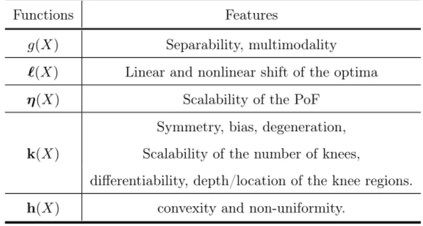
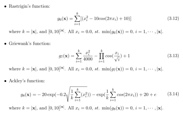
3.4.1 Landscape functions g(x) . . . 30

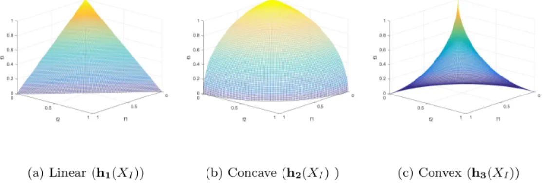
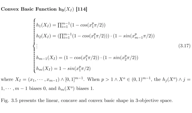
3.4.2 Basic Shape Functionsh(XI) . . . 33

3.4.3 Linkage Functions `(X) . . . 35

3.4.4 Knee Functionsk(XI) . . . 36

3.4.5 Stretching Functions η(x) . . . 39

3.4.6 Relationship Analysis . . . 40

3.4.7 Instantiations of Multi-objective Benchmark Problems for Knee De-tection . . . 47

3.5 Proposed Knee-oriented Performance Indicators . . . 48

3.6 Experiments and Analysis . . . 50

3.6.1 Experimental Settings . . . 50

3.6.2 Analysis of Proposed Indicators . . . 51

3.6.3 Discussions . . . 54

3.6.4 Explanations of Concerns on KD . . . 54

3.7 Summary . . . 56

4 An a Posteriori Knee-oriented MOEA based on Solution Set Augmen-tation 63 4.1 Introduction . . . 63

4.2 Proposed Framework . . . 65

4.2.1 Main framework of KSA . . . 65

4.2.2 Inverse Model . . . 67

4.2.3 Multimodal Auxiliary function transformation . . . 68

4.2.4 Meta-model . . . 69

4.2.5 Update Operation . . . 75

4.2.6 Peak Detection based Knee Identification (PD-KI) . . . 76

4.3 Experiments and Discussions . . . 79

4.3.1 Experimental Settings . . . 79

4.3.2 Investigations on KSA . . . 80

4.3.3 Comprehensive experiments on KSA and PD-KI . . . 84

5 An a Priori Knee Point Identification Based on Localized Bi-Dominance

Relationships 99

5.1 Introduction . . . 99

5.2 Proposed Bi-Dominance Relationships . . . 101

5.2.1 Related Definition . . . 101

5.2.2 Proposed Localized α-dominance Relationship . . . 103

5.2.3 Proposed Knee-oriented Dominance Relationship . . . 103

5.3 Investigation on the Knee-oriented Dominance Relationship . . . 106

5.4 An MOEA Driven by Localized Bi-Dominance Relationships (LBD-MOEA) 110 5.4.1 Overall framework . . . 110

5.4.2 Reference Vector Generation . . . 111

5.4.3 Update of Extreme Points . . . 112

5.4.4 Solution Association . . . 112

5.4.5 Bi-dominance Driven Environmental Selection . . . 113

5.4.6 Localized Knee-oriented-dominance based Selection . . . 114

5.4.7 Reference Vector Update . . . 120

5.4.8 Computational Complexity . . . 121

5.5 Experimental Results and Discussion . . . 122

5.5.1 Experimental Setting . . . 122

5.5.2 Performance Indicators . . . 124

5.5.3 Relationship Between Localized Bi-dominance Relationships and Pareto Dominance Relationship . . . 124

5.5.4 Sensitivity Analysis . . . 125

5.6 Experimental Results and Analysis . . . 129

5.6.1 Comparison with KGD Indicator . . . 129

5.6.2 Comparison with KIGD Indicator . . . 131

5.6.3 Comparison with KD Indicator . . . 132

5.6.4 Visualization of Results and Analysis . . . 133

5.7 Summary . . . 134

6 Hybrid Electrical Vehicle (HEV) Controller Design Problem 145 6.1 Introduction . . . 145

6.2 Investigation of KSA-MOEA and PD-KI on HEV Management Controller Design Problem . . . 150

6.3 Investigation of LBD-MOEA on HEV Management Controller Design Problem153 6.4 Summary . . . 156

7 Summary and Future Work 157

7.1 Summary . . . 157

7.2 Future Work . . . 159

1.1 The structure of thesis. . . 6

2.1 The knee point in convex region. . . 11

3.1 (a) An illustrative example of characters of knee regions. (b) An illustrative example how to mathematically calculate the width. . . 26

3.2 An example of non-differentiable knees on the PoF. . . 28

3.3 An illustrative example of the degenerated knee regions. . . 29

3.4 The mapping relationships of the proposed benchmark framework. . . 31

3.5 The shapes of the underlying PoF are formed by three different underlying shape functions in 3-objective objective space. . . 34

3.6 Examples on different settingski : (A, B, s),i= (1,· · · ,6)in knee functions k(XI) contribute to different PoFs. And p = 1 is set in the basic shape function h1, andη(x) = √ x on all objectives. . . 36

3.7 In (a) Example 1 and 2 plotm= (f(x) +f(y))/2andm=f(x)∗f(y)/2, re-spectively, wheref(z) = 5+10∗(z−0.5)2+cos(6πz)/2. Their corresponding contour lines are show in (b). . . 37

3.8 An example that illustrates the use of different stretching functions to change the scalability of the PoF. . . 40

3.9 PoFs given the settings (k2,h2) and the difference between them is the B values in knee function k2: (6, B,2). . . 41

3.10 PoFs: (A, B, s, p) with k1 : (6,1,−1)but (a) k1(XI) = [k1(x1)∗k1(x2)]/2, and p = 1 in h1(XI); (b) k1(XI) = k1(x1), and p = 1 in h1(XI); (c) k1(XI) = [k1(x1)∗k1(x2)]/2, and p= 2 inh1(XI). η(k1(XI)) = È k1(XI) on all objectives. . . 42

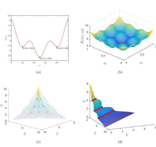
3.11 (a) shows the minima of k1(x). (b) shows the minima of k1(x1, x2). (c) shows the minima of k1(x1, x2) acting as the convex knees on the PoF. (d) shows the degenerated minima located in the degenerated convex regions. . 45

3.12 For all benchmark problems, X = [XI, XII] where XI : [0,1]|m−1| and

XII : [0,10]|n−m+1|, where nand mare the number of variables and

objec-tives respectively. The last two columns are the number of potential knees

according to the knee function. Ais one of the parameters in the knee

func-tions. x = k(XI) will change the scalability of PoF, and η(x) can be the

combinations between η1−η4 in Subsection IV-C on different objectives. . 46

3.13 Two examples to illustrate the difference between GD and KGD. . . 51

3.14 (a)-(d) present the solutions on PMOP1 with three objectives. (e) and (f) show the results on PMOP1 with 5 objectives, respectively. . . 52

3.15 (a) shows that P|_iK₌₁| d(νi,G) is not Pareto-compliant. (b) illustrates the second concern of KD. . . 55

3.16 The GD results obtained by six algorithms on PMOP test suite. . . 57

3.17 The KGD results obtained by six algorithms on PMOP test suite. . . 58

3.18 The IGD results obtained by six algorithms on PMOP test suit. . . 59

3.19 The KIGD results obtained by six algorithms on PMOP test suite. . . 60

3.20 The KD results obtained by six algorithms on PMOP test suite. . . 61

4.1 An example to illustrate the motivation. (a) plots the obtained solution set. (b) plots the augmented solution set where the red diamonds are the new solutions. . . 64

4.2 A flowchart of KSA. . . 66

4.3 An example is given to illustrate the multimodal transformation, whereF V is the distance information from solution to the hyperplane S constructed by the extreme points. The knee points are transformed to the minima of a multimodal auxiliary function (F V). . . 68

4.4 (a) The PoF of DEB2DK [15] is presented and the corresponding fitness curve of the PoF is obtained after the multimodal transformation. (b) The transformed multimodal function, the minima of which are correlated to the knee points of PoF. . . 69

4.5 Examples on DEB2DK [15] and CKP [138] problems to show the results after the operation of solution generation, where the given solutions are highlighted in green dots, and the new solutions are the blue diamonds. . . 75

4.6 An example to illustrate the peak detection to find the peaks of a multimodal function. . . 76

4.7 Two examples to show the ability of the peak detection to find the knee candidates on DEB2DK [15] and CKP [138] problems. . . 78

4.8 The increments of KIGD and KD values are presented in terms of the

in-crease of the number of evaluations. (a) and (b) are the KIGD and KD increment values in terms of the solution sets obtained before and after

4.9 The increments of different indicator values are presented in terms of the increase of the size of population obtained by RVEA. (a) and (b) are the KIGD and KD increment values in terms of the solution sets obtained before

and after KSA, respectively. . . 90

4.10 The increments of different indicator values are presented in terms of the increase of the size of population obtained by NSGA-II. (a) and (b) are the KIGD and KD increment values in terms of the solution sets obtained before

and after KSA, respectively. . . 90

4.11 The increments of different indicator values is obtained in terms of the given populations obtained by RVEA by running different number of generations. (a) and (b) are the KIGD and KD increment values in terms of the solution

sets obtained before and after KSA, respectively. . . 91

4.12 The increments of different indicator values is presented in terms of the population obtained by RVEA with the increase of the number of variables. (a) and (b) are the KIGD and KD increment values in terms of the solution

sets obtained before and after KSA, respectively. . . 91

4.13 The increments of different indicator values is presented in terms of the population obtained by RVEA with the increase of the number of objectives. (a) and (b) are the KIGD and KD increment values in terms of the solution

sets obtained before and after KSA, respectively. . . 92

4.14 An illustration of the experimental design. A population P is obtained by

an optimizer like RVEA after the maximum number of generations. KSA

is performed on P to get an augmented population A with the limit of

maximum number of evaluations, while population B inherits from P via

the same optimizer (RVEA) with the same maximum evaluations. . . 92

4.15 Experimental settings. Asymmetric and symmetric indicate the PoF is

asymmetrical or not. Nondifferentiable means that the knee is nondifferen-tiable. Unimodal and multimodal describe the difficulty in converging. Dis-continuous means that the PoF is complex and disconnected. Basic shapes are the PoFs where the knee functions are embedded on to create the knee regions. Maximum generations and evaluations are the stopping criterion

for the optimizer and proposed framework (KSA), respectively. . . 93

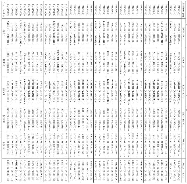
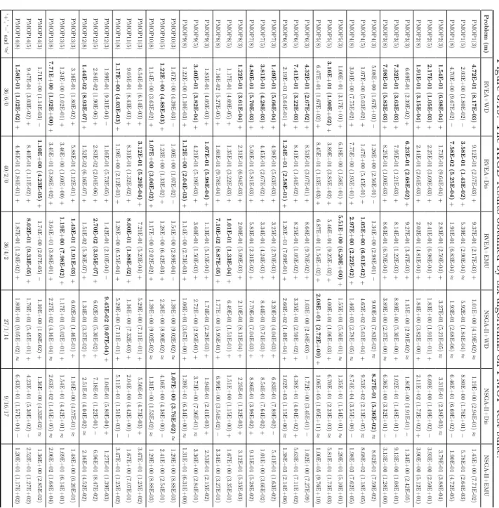
4.16 The KIGD values (average values, variance values) of the candidate so-lution sets obtained by the identification methods, and the corresponding increment values of the solution sets after the augmentation over the sets

before the augmentation of KSA. The best results are highlighted in grey. . 94

4.17 The KD values (average values, variance values) of the candidate solution sets obtained by the identification methods, and the corresponding incre-ment values of the solution sets after the augincre-mentation over the sets before

4.18 The KIGD values (average values, variance values) of the candidate solution sets obtained by the identification methods in terms of the augmented so-lution set acquired by KSA, and their corresponding increment values. The

best results are highlighted in grey. . . 96

4.19 The KD values (average values, variance values) of the candidate solution sets obtained by the identification methods in terms of the augmented so-lution set acquired by KSA, and their corresponding increment values. The

best results are highlighted in grey. . . 97

5.1 (a) An illustrative example of Pareto dominance and α-dominance, where

p1dominatesp3 in terms of both Pareto dominance andα-dominance, while

p1andp2 are non-dominated with each other in terms of Pareto dominance.

(b) An example of localized α-dominance, where the objective space is

di-vided into three subspaces by a set of reference vectors (L1, L2, L3). As

a result, solutions A and B are associated with L1, C and D with L2,

and E with L3. According to the conventional α-dominance, A and E are

non-dominated and the rest are dominated. According to the localized α

-dominance, however, A, C,D, and E are non-dominated with each other,

but B is dominated byA. . . 102

5.2 (a) – (e) illustrate different parameter α to the performance of localizedα

dominance based MOEA, , where the number of subspaces is set to six. . . 104

5.3 An illustrative example of the knee-oriented dominance relationship, where

φ is the acute angle between−−−→NidAand

−−→

AB, denoted byh−−−→NidA,

−−→

ABi. Here,

δ3 and δ2 are theminand max angles of solutionA . . . 105

5.4 (a) Illustration of three solutions and their dominated regions denoted by the

shaded area. (b) It is shown that more closer a solution to the hyperplane

is, the wider its dominated area will become. . . 105

5.5 An example to illustrate the relationship between angle γ and distance D

of solutionp. . . 107

5.6 An example to illustrate the relationship between the angles and knees,

where the knees correspond to the minima of the line (α+β). α and β are

themax and min ofδ of the solution on the PoF, respectively. . . 109

5.7 An illustrative example showing the importance of patitioning the objective

space into a number of subspaces in order to keep solutions in multiple knee regions. If the knee-oriented-dominance is used to compare solutions in the

whole objective space, solution A will dominate all solutions in the knee

5.8 (a)An illustration of the localized knee-oriented-dominance based selection on the critical front. Ten solutions are first grouped into four sub-populations, sorted separately using the knee-oriented-dominance, and assigned a sub-front number. The sorted solutions are combined again and sorted into three layers based on their sub-front number, where these layers consist of the solutions highlighted in different shapes and colors. Each solution is assigned with two numbers. The first number indicates the sub-population the solution is grouped into and the second number is its sub-front number.

(b) An illustration of the crowding distance, where A, B, C, D, E are the

solutions, and a, b, c, i, j, k represent the distances computed according to

the research [27]. . . 116

5.9 The KD values of the solutions obtained by KD-MOEA and NSGA-II over

the generations on PMOP2 with three, five, and eight objectives. . . 118 5.10 The KD values of the solutions obtained by LBD-MOEA and its variant

(LBD-MOEA*) over the generations on PMOP2 with three, five, and eight objectives. . . 118 5.11 The KIGD values of the solutions obtained by LBD-MOEA and its variant

(LBD-MOEA0) over the generations on PMOP2 with three, five, and eight

objectives. . . 120 5.12 Comparison of the performance of the knee-oriented dominance based

selec-tion on CKP with different settings of parameter τ. . . 121

5.13 The KGD, KIGD, and KD performance of LBD-MOEA over different num-bers of reference vectors. . . 128 5.14 The KGD, KIGD, and KD performance of LBD-MOEA on PMOP2 with

three, five and eight objectives. . . 128 5.15 The knee candidate solutions with median KD values obtained by seven

algorithms on DO2DK problems withK = 3. r(x)is the basic knee function

to control the shape and number of knee regions. . . 138 5.16 The knee candidate solutions with median KD values obtained by seven

algorithms on DEB2DK problems with K = 4. r(x) is the basic knee

function to control the shape and number of knee regions. . . 139 5.17 The knee candidate solutions with median KD values obtained by seven

algorithms on CKP problems with K = 5. r(x) is the basic knee function

to control the shape and number of knee regions. . . 140 5.18 The knee candidate solutions with median KD values obtained by five

al-gorithms on DEB3DK problems K = 3, respectively. r(x) is the basic knee

function to control the shape and number of knee regions. . . 141 5.19 The knee candidate solutions with median KD values obtained by the seven

algorithms on PMOP2 with 8 objectives. k(x) is the basic knee function of

5.20 The knee candidate solutions with median KD values obtained by the seven

algorithms on PMOP10 with 8 objectives. k(x) is the basic knee function

of PMOP10 to control the shape and number of knee regions. . . 142

5.21 The knee candidate solutions with median KD values obtained by the seven

algorithms on PMOP11 with 8 objectives. k(x) is the basic knee function

of PMOP11 to control the shape and number of knee regions. . . 142 5.22 The knee candidate solutions with median KD values obtained by the seven

algorithms on PMOP13 with 8 objectives. k(x) is the basic knee function

of PMOP13 to control the shape and number of knee regions. . . 143

6.1 The general architecture of the HEV, where the fuel and battery are the

power sources to the internal combustion engine (ICE) and electric motor (EM), respectively; the battery can be charged from the electricity grids or recharged during the braking; the request speed from the driver determines the torque generated by the electric motor; the HEV energy management controller controls the internal combustion engine by switching the operation

point in terms of the state-of-change (SOC) and current speedv(t). . . 146

6.2 An illustration of the architecture of the seven-objective HEV controller

model and its relationship to the optimizer as well as the HEV controller. . 147

6.3 (a) presents the obtained solution set obtained by RVEA before the

aug-mentation by KSA-MOEA. (b) plots the obtained solution set after the

augmentation by KSA-MOEA. . . 151

6.4 Plots (a) - (d) show the knee candidates obtained by EMUr, TKR, KnEA,

and PD-KI, respectively, before the augmentation by KSA-MOEA. Plots (e) - (h) present the knee candidates preserved by the four methods after the

augmentation. . . 152

6.5 Plots (a) - (d) show the boxplots of the knee candidates obtained by EMUr,

TKR, KnEA, and PD-KI, respectively, where all results are based on the solution set before the augmentation by KSA-MOEA. Plots (e) - (h) present the boxplots of knee candidates preserved by the four methods in terms of the solution set after the augmentation. The x-axis represents the number of solutions in the neighborhood (5, 10, and 15). The y-axis shows the number of solutions whose distances to the hyperplane are smaller than that of the

preserved solutions. . . 152

6.6 Plots (a) - (g) are the knee candidate solutions obtained by seven algorithms

on hybrid electric vehicle controller design problem. Plot (h) presents the approximated PoF of HEV controller design problem. (i) plots the potential knees of the approximated PoF. (j) presents the representative solutions in the corresponding knee regions. . . 155

Introduction

In traditional mathematical optimization [1], the optimization methods are deterministic and perform effectively on the unimodal optimization problems with good smoothness and most of them are gradient based approaches such as the Newton’s method and the hill climbing method [2]. However, their performances will seriously degrade if the gradient information with respect to different decision variables is unclear. Furthermore, many real-world optimization applications often involve multiple optimization objectives (criteria), and the objectives are commonly conflicting with each other. Accordingly, no single solu-tion can satisfy all objectives but a trade-off solusolu-tions can be found to the decision maker (DM) [3,4]. The traditional mathematical optimization methods also confront a great chal-lenge in dealing with such multi-objective problems which are nonlinear, non-differentiable or multi-modal.

However, the multi-objective evolutionary algorithms (MOEAs) have been demonstrated effective in dealing with such multi-objective optimization problems (MOPs) in the recent decades [4, 5]. The main reason is that such nature inspired algorithms do not need the gradient information during the optimization, and solutions can be identified even if many different objectives are considered at the same time. In the early research, the Pareto dom-inance based and aggregation based methods are popular, since they are able to provide a representative solution set with a good balance between the convergence and diversity towards the Pareto optimal front (PoF) of the MOPs [4]. However, when they are extended to deal with the MOPs with many objectives, the selection pressure towards the PoF

de-creases when the number of objectives inde-creases, and the diversity of the solution set also degrades significantly. Hence, different techniques are proposed to MOPs with many ob-jectives, such as the modifications on the dominance relationships, performance indicators based approaches, decomposition based approaches, diversity management enhancement driven approaches [6–8]. Interested readers are referred to Chapter 2.3 for more details of the development of MOEAs.

Although considerable progress has been made in research on many-objective optimiza-tions, some challenges remain to be addressed. For example, it will be impractical to represent the entire Pareto optimal front in a high-dimensional objective space using a relatively small number of solutions. In addition, it becomes increasingly challenging to select preferred solutions from the obtained solution set for the DM, and the preference articulation will be more difficult for many-objective optimization, because a large objec-tive space needs to explored and more trade-off information between the objecobjec-tives need to be considered. Last but not the least, most performance indicators measuring the dis-tribution of solutions no longer work properly in high-dimensional objective space since it is computationally extremely intensive to densely sample a high-dimensional space.

Due to the difficulties discussed above, it is more practical to concentrate on potentially interesting regions in solving MOPs with many objectives. To this end, preference driven MOEAs provide an effective means to focus on the search of solutions of interest [9] and are computationally more efficient [10, 11]. If user preferences are available, we can use them to guide the search towards the regions of interest (ROIs) [9], thereby making it easier for the DM to select a small number of solutions for final implementation [12]. For the above reasons, preference based evolutionary optimization algorithms have attracted much research interest in the past decades [7, 13]. Interested readers are referred to Chapter 2.4 for more details of the preference-driven approaches.

However, several concerns have been raised regarding the preference-driven approach [14]. Firstly, explicit preferences may be hard to be articulated beforehand, if the decision-maker

do not have sufficient a priori knowledge of the problem. Secondly, it is not

straightfor-ward to articulate the preferences during the optimization and interactively tuning the preferences during the optimization may be arduous and sometimes intractable. Thirdly,

it is resource-intensive in thea posterior approach to acquire a representative solution set over the whole PoF, especially when the number of objectives is large and the shape of the PoF is highly complex.

Accordingly, the search of naturally preferred solutions such as the knee points becomes

attractive when the DM does not have sufficienta priori knowledge of the problems. The

knee points are the solutions on the PoF, which need a large compromise on at least one objective to achieve a small amount increase in other objectives [15]. It has also been shown that knee solutions contribute to a larger hypervolume in comparison with other Pareto optimal solutions [16]. In addition, knee points have been successfully used to deal with a range of problems, such as self-adaptive software [17], dynamic optimization [18], many-objective optimization problems [19], sparse reconstruction [20], and driving strategy for electric vehicles [21]. Interested readers are referred to Chapter 2.5 for more details of the knee oriented approaches.

The remainder of this chapter is organized as follows. The challenges is firstly presented; afterwards, the main contributions of the thesis are detailed; finally, the structure of this thesis is introduced.

1.1

Challenges

When the user-preference is unavailable, there are still some challenges in the search of the natural interesting solutions like the knees or solutions in the knee regions of the PoF.

Difficulty in evaluating the performance of the knee-oriented approaches. Few

benchmark problems have been designed to systematically assess the ability of an opti-mization algorithm to find knee points with few exceptions, including the DO-DK and DEB-DK problems [15, 22]. Note that DO-DK and DEB-DK problems did not consider many important characteristics of knee points such as the positions of the knees, different geometric shapes of the PoF, bias, separability, degeneration of the knee regions, differen-tiability of the knees, scalability of the PoF, and symmetry of the knee regions. Besides, there are no available indicators for the performance evaluations.

Difficulty in acquiring diverse solutions in high-dimensional objective space

when to find the knee candidates in an a posteriori way. Existing identification

methods may have good performance in characterizing the knee candidates among a large number of solutions when the given solution set is well converged and well distributed in the knee regions. In practice, it is difficult to acquire a sufficiently large set of solutions to represent the entire PoF for problems having a large number of objectives due to the limited computing resources [14]. Accordingly, the performance of most knee identification algorithms will seriously degrade if the given solution set has a very small number of solutions distributed in a knee region.

Challenge in effectively locating the knee regions in high-dimensional objective

space in ana prioriway. A priori searching the knee regions to the DM may be a good

line of research, which can facilitate the decision making with only the interesting knee candidates and save computing resources by focusing the search in knee regions rather than the whole PoF. However, the uninterested solutions (such as the extreme points, boundary solutions, or solutions in the concave regions) are hard to be eliminated during the optimization and they may easily become the dominance resistance solutions which can slow down the convergence rate and mislead the search process. Furthermore, it is difficult to balance the search of more knee regions and better convergence of the population toward the knee regions of the PoF.

As a consequence, the motivation of this thesis is to tackle the above challenges, and the main contributions are listed as follows.

1.2

Main Contributions

A knee-oriented benchmark test suite and indicators. A benchmark test suite is

proposed to assess the performance of MOEAs in the search of knee candidates of MOPs. When the preference information is unavailable, the knees or knee regions on the PoF are natural preference for MOEAs. As a consequence, such a test suite is very necessary, which can comprehensively evaluate the performance of MOEAs in the search of knee or knee regions of MOPs and MOPs with many objectives. Besides, relevant knee-oriented indicators are also proposed.

A knee-oriented solution augmentation strategy fora posterioriknee

identifica-tion. An solution augmentation strategy is proposed to augment the given solution set by

generating solutions near the promising knee regions, thereby improving the performance of thea posterioriknee identification methods. Although a number knee identification meth-ods are effective in search of knees, most research performs knee identifications on a set of Pareto optimal solutions, implicitly assuming that the solution set is well-distributed and able to cover all the knee regions. However, this assumption may fail in practice, because it is challenging to get a large size of solution set covering the whole PoF, especially when the PoF is complex and high-dimensional. Hence, this work is to alleviate the concern of the assumption.

Localized Bi-dominance relationships driven MOEA for a priori knee

identifi-cation. An novel MOEA is proposed fora priorilocating knee regions of MOPs and MOPs

with many objectives by means of the proposed two localized dominance relationships. It is known that identifying all convex knee regions of a Pareto front is extremely challenging, especially in high-dimensional objective space. One the one hand, the optimization process needs to be guided towards the PoF. On the other hand, diverse knee regions also need to be taken into account. Consequently, this study puts up with a new line of research of knee detection by introducing localized dominance relationships in high-dimensional objective space.

1.3

Structure of Thesis

According to the Fig. 1.1, the structure of the thesis is shown as follows.

• Chapter 2 mainly introduces the background knowledge of the thesis. Specifically, the

definitions of multi-objective or many-objective optimization problems, Pareto dom-inance relationship are first provided. Then, literature reviews of different categories of MOEAs are presented, including the dominance-based approaches, performance indicators based approaches, decomposition based approaches, diversity management enhancement based approaches, especially, the preference-assisted approaches. Fur-ther more, the evolutionary optimization for knee identifications is detailed. Finally,

Background: Problem, Definitions, MOEAs, Knee identifications, Benchmarks

Chapter 2

Chapter 6 Chapter 7

Chapter 3 Knee-oriented benchmarks and indicators

Bi-localized dominance relationships

driven MOEA for apriori knee detection

Chapter 4 Chapter 5

Real application: hybrid electric vehicle controller design

Summary and future work An a Posteriori Solution augmentation for knee identification

Figure 1.1: The structure of thesis.

some benchmarks for evaluating the performance of MOEAs are introduced.

• Chapter 3 details the proposed knee-oriented benchmarks and indicators which are

designed for the test of the knee detection or identification. At the beginning, relevant studies on building benchmarks are introduced. Then the way to construct the knee-oriented benchmarks are proposed, followed by three indicators. Empirical results on the benchmarks are presented and discussed.

• Chapter 4 details the solution augmentation strategy for knee identification. To begin

with, the framework of the strategy how to augment the solution set is elaborated step by step. Then a knee detection method based on the strategy is introduced. Some analyses on the strategy and knee detection are exhibited. Finally, performance verifications are conducted on a variety of benchmarks.

• Chapter 5 details the bi-localized dominance relationships driven MOEA for knee

the localized knee-oriented dominance. Afterwards, an MOEA based on these two dominance relationships is presented. Finally, the sensitive analysis and performance evaluations on the algorithm is conducted.

• Chapter 6 firstly introduces a real application, i.e., hybrid electric vehicle controller

design problem. Then some experiments are conducted on the application to verify the effectiveness of the proposed methods proposed in Chapters 4 and 5.

• Chapter 7 summarizes the thesis and introduces some lines of research for future

study.

1.4

List of Publications

Guo Yu, Yaochu Jin, Markus Olhofer, Qiqi Liu, Solution set augmentation for knee

iden-tification in multiobjective optimization. IEEE Transaction on Evolutionary Computation,

2020. (Under review)

Guo Yu, Yaochu Jin, Markus Olhofer, A multi-objective evolutionary algorithm for finding

knee regions using two localized dominance relationships. IEEE Transaction on

Evolution-ary Computation, 2019. (Major revision)

Guo Yu, Yaochu Jin, Markus Olhofer, Benchmark problems and performance indicators

for search of knee points in multiobjective optimization. IEEE Transactions on

Cybernet-ics, 2019. (In press)

Guo Yu, Yaochu Jin, Markus Olhofer, References or preferences – rethinking

many-objective evolutionary optimization. In Proceedings of 2019 IEEE Congress on

Evolu-tionary Computation (CEC), 2019. (In press)

Guo Yu, Yaochu Jin, Markus Olhofer, An a priori knee identification multi-objective

evolutionary algorithm based onα-dominance. In Proceedings of the Genetic and

Evolu-tionary Computation Conference 2019 (GECCO’ 19 Companion). ACM, New York, NY, USA, 2019. (In press)

Guo Yu, Yaochu Jin, Markus Olhofer, A method for a posteriori identification of knee

Computation (CEC), 1-8, 2018.

Qiqi Liu, Yaochu Jin, Martin Heiderich, Tobias Rodemann, Guo Yu, An adaptive

ref-erence vector guided evolutionary algorithm using growing neural gas for many-objective

optimization of irregular problems, IEEE Transactions on Cybernetics, 2020. (Under

re-view)

Jianpeng Long, Xiaojun Zhou, Yaochu Jin, Guo Yu, Chunhua Yang, Fast constrained

Background

2.1

Problem Formulation

Definition 1 (Multiobjective optimization problem) Without loss of generality, a

multi-objective optimization problem can be formulated as the minimization ofm objectives1:

minimize F(x) = (f1(x),· · ·, fm(x))T, s.t. x∈_X, F∈_Y,

(2.1)

wherex= (x1,· · ·, xn) is the decision vector. X⊆Rn is the decision space, andn is the

number of decision variables. F:X→Yconsists ofmobjectives. Y⊆Rm is the objective

space. Whenm= 2 or 3, the problem is referred to as a multi-objective problem (MOP);

ifm≥4, as a many-objective problem (MaOP).

Definition 2 (Pareto dominance) Given two solutions x1,x2 ∈ X, x1 is said to Pareto

dominatex2, denoted byx1≺x2, if and only if the following equation is satisfied:

∀i∈ {1,2, . . . , m}, fi(x1)≤fi(x2)

∧ ∃j∈ {1,2, . . . , m}, fj(x1)< fj(x2).

(2.2)

A solution is Pareto optimial if there is no feasible solution can Pareto dominate it. The collection of all Pareto optimal solutions in the decision space is the Pareto set (PS), and

1_{Maximization problems can be equivalently transformed to minimization problems by taking negative}

its corresponding collection in the objective space is dented by the Pareto optimal front (PoF).

Definition 3 (Pareto-optimal set and Pareto-optimal front) In problem (2.1), the set

X⊂Xof all the nondominated solutions is called the nondominated or Pareto-optimal set

(PS). The Pareto-optimal front (PoF) is the image of PoS in the objective space [4].

Definition 4(Multimodal optimization problem) Without loss of generality, a multimodal

optimization problem (MMOP) involving multiple maximum solutions of a single objective can be formulated as the maximization of an objective function:

maximize f(x),

s.t. x∈X,

(2.3)

wheref(x) is the objective function, andx= (x1,· · ·, xn) is the decision vector and nis

number of decision variables.

The global optimal solution setX∗ of Problem (2.4) can be stated as follows:

X∗={x|_@y∈X :f(y)< f(x)∧y6=x}, (2.4)

where|X∗|>1.

2.2

Generically Preferred Solutions

Generally speaking, knee points, edge knee points, extreme points, and robust solutions [23, 24] are solutions generically preferred by users. In the following, we mainly discuss in detail the main properties of knee points and knee regions. Knee points, which require large sacrifices in at least one objective to gain a small amount of improvement in another objective [23, 25]. In this work, only the knees in the convex regions [26] are considered.

Definition 5In [26], a knee point in a convex region of a PoF is defined with the maximum

distance from the convex hull of individual minima (CHIM) to the hyperplane constructed by the extreme points.

k= arg max

f1 A B ˆ n S_ N_B I p z

p

Figure 2.1: The knee point in convex region.

wherep is a solution on the PoF. d(z(p), S) denotes the distance from solution p to the

hyperplaneS :f1+· · ·+fm= 1 in a normalized coordinate system.

In the normalized coordinate system, as shown in Fig. 2.1, the knee pointpz = arg max

pi

(|ti|· k ˆ

nk), wherenˆ is the orthogonal basis of the boundary line S_N BI, and |ti|is the distance

from normalized solutionpi to S_N BI.

2.3

Multi- and Many-objective Evolutionary Optimization

Evolutionary algorithms are population based algorithms inspired by the natural evolution. Given an optimization problem, a population of solutions are generated according to the problem, then a series of evolutionary operations are conducted on the population, such as the crossover, mutation, and selection operators in each generation (iteration). In each generation, offspring population is generated based on the elite solutions (solutions with better fitness values) among the parent population. As a result, the population evolves to better solutions to the optimization problem.

Over the last decades, many algorithms have been developed in both multiple criteria decision making (MCDM) community and the evolutionary computation community that are capable of finding a set of well-distributed solutions approximating the Pareto optimal front (PoF). Earlier popular multi-objective evolutionary algorithms (MOEAs) for dealing with MOPs are mainly Pareto dominance based and weighted sum approaches. The Pareto

dominance-based approaches include the non-dominated sorting genetic algorithm (NSGA-II) [27], the strength Pareto evolutionary algorithm (SPEA2) [28], and the niched Pareto genetic algorithm (NPGA) [29]. Examples of the weighted sum approaches are genetic algorithms with variables weights [30] and dynamic weighted aggregation evolution stratgy [31].

However, when the Pareto-dominance assisted algorithms are extended to solve MaOPs, they will fail to find a representative solution set with a good balance between the con-vergence and diversity. It is attributed to the loss of selection of pressure towards the PoF. Specifically, the Pareto-dominance cannot distinguish the relationship between the solutions in high-dimensional objective space [32], because the solutions are non-dominant with each other in the high-dimensional objective space. The weighted sum approaches are ineffective in solving MOPs with a non-convex shape of the Pareto front. The reason is that the solutions in the extreme regions or boundary regions always have larger utility values (aggregation values) than other solutions, which lead to serious degradation of the diversity performance of the solutions. In other words, the solutions from the extreme regions or boundary regions have higher priority to be selected than others during the en-vironmental selection and much more selection pressure are guided towards these regions other than the center area of the PoF.

To address the above issues, the multi-objective evolutionary algorithms (MOEAs) pro-posed for solving MaOPs can be roughly categorized into four groups, i.e., dominance relationship based approaches, performance indicators based approaches, decomposition based approaches, and diversity management enhancement driven approaches [6–8].

2.3.1 Dominance Relationship based Approaches

The first group of approaches aim to increase the selection pressure of the population towards the PoF by modifying the traditional Pareto dominance relationship, such as enlarging the dominant areas of a solution. Accordingly, the efficiency in distinguishing the relationship between the non-Pareto dominant solutions are significantly improved.

Laummans et al. [33] first propose the -dominance to extent the dominating area of a

et al. [34], which is integrated into a steady-sate algorithm (-MOEA). The bigger the is, the larger dominated area of a solution will have. To tackle another issue that the

dominance resistant solutions (DRSs) 1 seriously degrade the convergence of the

popula-tion when the Pareto dominance relapopula-tionship is used for solupopula-tion comparison, Ikedaet al.

proposed a modified dominance relationship, which is named asα-dominance [35]. When

two Pareto non-dominant solutions are compared, the α-dominance favors the solution

having at least one objective substantially superior than that of its peer solution. Batista

et al. leveraged the advantage of the-dominance and theα-dominance, and proposed the

cone-dominance. Recently, Yang, et al. proposed a grid dominance based evolutionary

algorithm (GrEA) [36], where solutions in the objective space are transformed into a grid coordinates for the comparison during the environmental selection. The grid dominance also favors solutions having substantially superior objectives. There are a number of other modifications of Pareto dominance relationships, such as the angle-dominance [37], fuzzy dominance [38], preference order ranking [39], and other ranking methods such as [40, 41].

2.3.2 Performance Indicators based Approaches

The second group of approaches aim to select solutions based on existing performance indicators or metrics. During the environmental selection, the fitness of a solution can be expressed by the indicators with respect to the convergence performance, diversity performance, or comprehensive performance.

The S metric or hypervolume (HV) [42] is a performance metric which is widely used to

evaluate the comprehensive performance of an algorithm with respect to both convergence and diversity performance of the obtained solution set. For example, the indicator based evolutionary algorithm (IBEA) [43] predefines a goal of each solution to measure its

contri-bution withindicator [44] or hypervolume (HV) indicator [42]. Both S metric selection

evolutionary multi-objective optimization algorithm (SMS-EMOA) [45] and hypervolume estimation algorithm (HypE) [46] are based on HV. But SMS-EMOA calculates the exact contribution to hypervolume indicator while HypE assigns a fitness based on approxima-tions to the hypervolume indicator. The main advantage of the HV based methods is not

1_{In [35], the DRSs are defined as the solutions which are extremely inferior in at least one objective}

being subject to the problems that the pareto-dominance based MOEAs encounter, but their computational cost is relatively expensive. Recently, some other metrics are also

adopted to efficiently deal with the MaOPs. For example, Menchaca-Mendez et al. [47]

proposed a GD indicator based MOEA (GD-MOEA for short), which is improved by

intro-ducing the-dominance into GD-MOEA to deal with MaOPs (termed GDE-MOEA) [48].

Trautmann et al. developed R2 indicator [49] and Gómez and Coello [50, 51] extended

the R2 indicator to many-objective optimization. Recently, Schutzeet al. [52] proposed a

performance measure (“averaged Hausdorff distance”) for multiobjective evolutionary

opti-mization. Yeet al. proposed an enhanced inverted GD (IGD) [53] and adopted the metric

for dealing with MaOPs [54].

2.3.3 Decomposition based Approaches

The third group of approaches aim to divide an MOP or MaOP into a number of subprob-lems and then solve them simultaneously [55, 56]. Generally, there is an hypothesis behind these approaches that the references or preferences information used in these approaches are able to guide the search process toward the subregions of the PoF, and the subregions can represent the whole PoF.

To this end, the category of the decomposition based approaches is not limited to the approaches only using the decomposition or aggregation methods but also the approaches using reference information. Both MOEA/D [55] and MSOPS [57] are the representa-tive decomposition methods, and they decompose MaOP into a set of subproblems via the scalar functions (weighted sum approach [4], Tchebycheff approach [4], or penalty-based boundary intersection (PBI) approach [55]). Then the subproblems are simultane-ously optimized to obtain the optimal solutions constituting a representative subset of the Pareto optimal front (PoF). Another class of methods adopts reference vectors or reference points to guide the optimization towards different subregions of the PoF, then simultane-ously search the optimal solutions of the subregions, such as the reference vector guided evolutionary algorithm (RVEA) [58], nondominated sorting genetic algorithm III

(NSGA-III) [59], MOEA/dominance and decomposition (MOEA/DD) [60], andθ-dominance based

(MOEA/D-M2M) [62].

In [63], the differences and similarities between the preference and reference driven ap-proaches are detailed and discussed.

2.3.4 Diversity Management Enhancement Driven Approaches

The last group of approaches are known as the diversity management enhancement driven approaches. In many-objective optimization, the solutions are distributed very sparse while the diversity management becomes particularly useful in the environmental selection as it may reduce the negative impact from the excessive diversity to the convergence of the population.

In [64], Adra and Fleming proposed the diversity management operator (DMO) which is to maintain the diversity until the solutions converge into the Pareto optimal front.

Recently, Liet al. proposed a shift-based density estimation strategy [65] to penalize poorly

converged solutions by assigning them a high density value. As a result, the candidate solutions with a good balance between convergence and diversity can be sorted out and

added into the next generation. In [66], Wang et al. proposed a coevolution strategy

based MOEA, where the preference coevolves with respect to the diversity performance

of the solution set. Wang et al. introduced two-archive strategy [67] to maintain the

diversity and convergence of the population. Yu et al. proposed boundary elimination

selection [68] to tackle the DRSs and maintain the diversity of the population in

many-objective optimization. Zhang et al. proposed a knee-point driven MOEA [69] which

choose the candidate knee points during the environmental selection, because the knee points contribute much more on the HV than other solutions.

2.4

Preference-assisted Evolutionary Optimization

Although the proposed approaches made great progress in dealing with MaOPs, some issues remain to be resolved [63]. For example, it has been demonstrated that the performance of the aggregation-based approaches strongly depends on the shapes of the PoFs [70]. The performance of the reference-based methods also depends on the distribution of the

predefined references [58] because the predefined subproblems may waste computational

resources and fail to explore some sub-regions. In dealing with MOPs, a manageable

number of solutions is able to present a good approximation to the PoF. However, it is hardly practical when the same population size is adopted in dealing with MaOPs. The performance indicators may introduce biases in specifying the reference points [71]. Thereby, finding regions or solutions of interest by introducing the user-preference into the searching process is more practical [9]. Moreover, more computing resources can be saved [10] and the tricky decision making can also be simplified since the obtained solutions are from the regions of interest rather than the whole PoF [11, 72]. Accordingly, much at-tentions have been paid to developing preference-driven approaches to deal with MOPs or MaOPs. In preference-based methods, there are different types of preference articulations, such as goal attainment [73], weight vectors [10, 66, 74], reference vectors [75–78], prefer-ence relations [79–81], fuzzy preferprefer-ences [82], utility functions [83–85], outranking [86, 87], extreme points or the nadir point [88, 89]).

Depending on when the DM intervenes the search process, ie., before, during or after the search process, the “human-in-the-loop” approaches can be classified into three cate-gories, namely, a priori, interactive and a posteriori methods. The details integrating the preference into multi-criteria decision making (MCDM) and evolutionary multi-objective optimization (EMO) methodologies are reviewed in [7,73,90,91]. Among these three meth-ods, the a priori and interactive methods are particularly appealing, and have been adopted by several algorithms hybridizing EMO and MCDM methods. Branke [92] and Deb [93] proposed a guided multi-objective evolutionary algorithm (G-MOEA) based on modified dominance relationship upon the DM’s preference information. Deb et al. integrated the reference point [76] and reference direction [94] into the interactive EMO algorithm respec-tively. Besides, Thiele et al. [95] suggested reference point based EMO procedures to find a set of points close to the specified multiple reference points. Molina [96] and Ben [97]

proposedg-dominance relationship andr-dominance relationship respectively, which both

modified the Pareto-dominance relationship with the reference point, but the former fo-cuses on one reference point and is based on a priori; the later is one sort of multiple reference points based interactive method. Interested readers are referred to [7, 13] for more details of the preference-driven approaches.

Accordingly, when the DM has enough a priori knowledge, the preference-driven ap-proaches are promising in the search of solutions of interest for the DM.

2.5

Evolutionary Optimization for Knee Identifications

When user preferences are not available, the preference-driven approaches confront a big challenge. However, the knee points are considered as the preferred solutions, since they need a large compromise in at least one objective to gain a small improvement in other objectives [23,98]. Besides, knee solutions are often prioritized in many MOEAs since they usually contribute to a large hypervolume [69]. Many algorithms have been proposed by taking advantage of knee solutions to more efficiently solve MaOPs [19, 69] or dynamic optimization problems [18]. Knee solution based MOEAs have already found successful applications in solving real-world problems, such as self-adaptive software [17], sparse re-construction [20], and driving strategy for electric vehicles [21].

In consequence, severala posteriori methods have been proposed to characterize the knee

points among a set of non-dominated solutions. Das et al. [26, 99] suggested to identify the knee points with the “maximum bulge” on the Pareto front using the normal boundary intersection [100]. Branke et al. [15] took advantage of the expected marginal utility (EMU) to locate the knee regions. The niching method [101] defines possible knee points in convex and concave regions based on the density of the solution distribution. Other methods have also been reported for identifying the knees of two-objective problems, such as the

reflex/bend angle based approaches [15, 102], and its variant, the (α, β)-approach [23].

Notably, there is an assumption in alla posteriori approaches that a large set of well

dis-tributed and well converged solutions is available. However, it is computationally expensive

to achieve such a solution set, especially for MaOPs. Therefore, a priori approaches to

the search of knee regions are popular. For example, in [103, 104], methods for charac-terizing knee points with the max-min utility value is incorporated in the environmental selection. However, the boundary points usually have a larger utility value than other solutions and will most likely be kept in the environmental selection, which may mislead the search process. Zhang et al. developed a selection method for solving MaOPs by prior-itizing knee points [69] identified based on the extreme points [26]. However, the extreme

solutions may become dominance resistant solutions (DRSs) [35] that will seriously slow down the convergence of the population. In [35], the DRSs are defined as the solutions which are extremely inferior in at least one objective and there exist very few solutions that are able to dominate them. The work in [105] recursively uses the EMU [15] to locate the most promising knee candidates during the environmental selection. However, this approach also favors the boundary points and DRSs in the search, which degrades the convergence performance. The angle-based pruning strategy [106] was adopted to detect the knee regions [107] in the environmental selection, although the issue of DRSs remains.

Most recently, we introduced anα-dominance to eliminate the DRSs for the search of knee

solutions [108]. However, uninterested solutions like the boundary points and solutions from the concave knee regions will still be selected. Too much convergence pressure of the modified dominance may degrade the diversity of the solutions by eliminating the knee candidates in a potential knee region, so that less knee regions will be finally preserved. A common issue is that some particular solutions, such as some extreme and boundary solutions, are detrimental to the effective search of knee solutions. Another issue is how to

effectively and efficiently locate the knee regions in ana prioriway. Against the assumption

above, there is always no representative solution set provided in practice to cover the whole PoF for the knee identification. Therefore, there are big gaps to fill in the searching of knee regions.

2.6

Existing Benchmarks

To evaluate the performance of the MOEAs in dealing with the MOPs and MaOPs, the test suites are used for empirical studies. The ZDT [109], DTLZ [110], and WFG [111,112] test suites are widely used for the studies on MOPs and MaOPs. Especially, the DO-DK and DEB-DK problems are widely used for evaluating the performance of MOEAs in search of specific regions of interest like the knee regions.

K. Deb, L. Thiele, and E. Zitzler proposed ZDT [109] and few years later they and E. Zit-zler proposed another set of test suites DTLZ [110] which are widely used to evaluate the performance of the EMO algorithms. ZDT test suite is mainly for the evaluation of the

ability of the convergence and diversity. Three basic functions are introduced in the con-struction. The position/distribution function (normally the first objective function) with or without bias controls the distribution of solutions along the PoF; the distance function with or without multimodal/unimodal tests the ability of the algorithm converging to the PoF; the shape function determines the final shape of the PoF (convex, concave, or discon-nection). Except binary-coded ZDT5, ZDT1-4 and ZDT6 are real-coded designs to test the convergence and diversity of EMO algorithms. However, the limitation of ZDT suite is that they are all bi-objective. Further on the ZDT test suite, DTLZ test suite is developed with flexible scalability on objectives and variables. All of the problems can be scaled to any number of objectives and decision variables and they are able to test different aspects of the algorithms by providing different challenges. The suite can be divided into two groups. The first group involves DTLZ2, DTLZ4, DTLZ5 and DTLZ7, which are designed to test algorithms’ ability to address the problems with different shapes and locations of Pareto optimal front (PoF). The second group consists of DTLZ1, DTLZ3, and DTLZ6, which create more obstacles to impede the solutions converging into the PoFs.

The Walking Fish Group (WFG) test suite [111, 112] has a flexible design, and provides a variety of predefined shape and transformation functions to change the difficulty and features of the problems. About the construction, WFG toolkit designs an underlying

vector (x) associated with an underlying problem to define the fitness space. By a series

of transition mapping functions, the working parameters (z) are transformed to x, and

each transition function represents different complexity such as multimodality and non-separability. Particularly, in the construction of WFG problems, the toolkit only requires to specify different settings on the parameters of the shape functions and transition func-tions to define the PoF as well as the fitness space respectively. WFG1-2 have convex PoFs; WFG3 has a linear degenerate PoF; others are concave. WFG1,WFG7-9 have biased PoFs. WFG2-3, WFG6, and WFG8-9 have nonseparable fitness landscape. WFG5 and WFG9 are deceptive. WFG is a continuous problem suite that can be scaled to any number of ob-jectives and decision variables. Comprised of problems with various characteristics (such as having linear, convex, concave, multimodal, disconnected, biased, and degenerated Pareto fronts), the WFG suite is used to challenge varying capabilities of an EMO algorithm. In [15, 22], five benchmark problems are proposed, including two bi-objective problems

(DO2DK, DEB2DK) and one 3-objective problem (DEB3DK) and two MaOPs (DEB4DK, DEB5DK) with 4 and 5 objectives. The problems in [15, 22] only considered the symmetry PoF with knees on hyperplane, not considering some features commonly seen in real-world problems (asymmetry PoF, multimodality in fitness landscape, variable separability, variable linkage, differentiability, degeneration, different locations of knees, robustness). Besides, different features on the knees need to be taken into account, such as different biases could cause the shift of the knees; different settings could cause the degeneration of knee regions; different parameter settings could cause symmetry and asymmetry; the knees are differentiable or non-differentiable; also the degeneration of the knee regions. For DMs, they would like to see a robust algorithm having different strong abilities. Thus, on the one hand, the benchmarks should be designed more close to real applications; on the other hand, the benchmarks should test different aspects of the problems simultaneously. However, less benchmark problems can be adopted to comprehensively test the ability of the methods finding preference on the MOPs and many-objective optimization problems except DO2DK and DEB2DK [15, 22]. But the variance and scalability of them [15] are limited. Specifically, different positions of the knees, different geometric shapes of the PoF, bias, separability, degeneration of the knee regions, robustness of the knees, and differentiability of the knees are not taken into consideration for the testing.

Benchmark Problems and

Performance Indicators for Search of

Knee Points

3.1

Introduction

Although a variety of test problems have been reviewed in Section 2.6 of Chapter 2, few benchmark problems have been designed to systematically assess the ability of an opti-mization algorithm to find knee points with few exceptions, including the DO-DK and DEB-DK problems [15, 22]. Note that DO-DK and DEB-DK problems are designed only for identifying knee points without considering many important characteristics of knee points such as the positions of the knees, different geometric shapes of the PoF, bias, sep-arability, degeneration of the knee regions, differentiability of the knees, scalability of the PoF, and symmetry of the knee regions.

This study is motivated by the fact that few knee functions, benchmark problems and performance indicators have been proposed to test and assess the performance of MOEAs in approximating knee points of multi- and many-objective optimization problems in terms of the number of the knee points found, their accuracy and location. To fill the gap, we propose five new basic knee functions and a new construction method of knee functions.

Furthermore, a set of new benchmark problems are constructed using the proposed knee functions whose Pareto fronts have various characteristics in symmetry, differentiability

and degeneration. Apart from these properties directly related to knee regions, other

challenges in solving optimization problems such as multi-modality, non-uniformity and linkage in decision variables are taken into account. Meanwhile, performance indicators for evaluating various aspects related to MOEAs’ performance in identification of knee points of complex Pareto fronts are suggested.

The rest of the chapter is organized as follows. Section 3.2 provides a concise review of existing benchmark problems. Section 2.2 elaborates various features of Pareto optimal solutions considered in construction of the test problems. Section 3.4 presents the details for constructing the proposed benchmark problems, followed by a description of the proposed metrics in Section 3.5. The experiments and analysis are conducted in Section 3.6. Finally, Section 3.7 concludes the chapter.

3.2

Related Work

In this section, we briefly review existing popular benchmark problems based on which this work is built.

3.2.1 ZDT and DTLZ Problems

The ZDT [109] and DTLZ [110] test suites are most widely used multi-objective optimiza-tion benchmark problems constructed for evaluating MOEAs. The construcoptimiza-tion of both test suites is based on the bottom-up approach [110], which allows for separately design of the objective functions, the decision space, and the Pareto-optimal front. Specifically, decision variables are divided into position and distance variables, which define the Pareto front and determine the distance of the solutions to the PoF, respectively. The ZDT test suite is constructed in the following form:

min

x :z(x) = (f1(x1), f2(x))

subject tof2(x) =g(x2,· · ·, xn)h(f1(x1), g(x2,· · · , xn))

wherex= (x1,· · · , xn)∈Ω

In the above construction, x1 is the position variable and the rest are the distance

vari-ables. The ZDT test problems are constructed using three basic functions, namely, the

position/distribution function f1 with or without bias for controlling the distribution of

Pareto optimal solutions along the PoF, the uni- or multi-modal distance function g for

testing the algorithm’s ability of converging to the PoF, and the shape function h for

determining the convexity and continuity of the PoF.

The DTLZ test suite [110] was developed based on the ZDT test functions in order to enhance the scalability to the number of decision variables and objectives. The DTLZ test suite is constructed as follows:

min

X :fi=1:m(X) = (1 +g(XII))·hi(XI).

whereX= (XI, XII)∈Ω

XI = (x1,· · · , xm−1), XII = (xm−1,· · ·, xn)

(3.2)

where, XI in the shape functions h1:m(XI) are the position variables determining the

geometry of the PoF while XII are the distance variables embedded in the landscape

functions to control the closeness of the Pareto optimal solutions to the PoF, wherem is

the number of objectives.

Note, however, that neither ZDT nor DTLZ pays particular attention to the complexity of the PoF, and it is assumed that there is no correlation between the position and distance variables.

3.2.2 WFG Problems

The design of the WFG problems [111, 112] also follows the bottom-up approach [110] but differs from the approach to designing the ZDT and DTLZ test suites. The construction of the WFG test suite is as follows:

Givenz={z1,· · ·, zk, zk+1,· · ·, zn} min x :fi=1:m(x) =xm+Sihi(x1,· · · , xm−1) x={x1,· · ·, xm}={max(tpm, A1)(tp1−0.5) + 0.5,· · ·,max(t p m, Am−1)(tpm−1−0.5) + 0.5, t p m} tp={tp₁,· · · , tp_m} ←[tp−1 ←[· · · ←[t1 ←[z_[0,1] z_[0,1]={z_1,[0,1], . . . , z_n,[0,1]}={z1/z1,max,· · ·, zn/zn,max} (3.3)

The WFG test suite is used for constructing a problem in terms of an underlying vector

of decision variablesxderived from a series of transition vectorst1:p, where the transition

vectors are derived from a vector of working parameters z. Each transition vector can

add complexity to the underlying test problem, such as non-separability, multimodality,

deception, and bias. S1:m >0 and A1:m−1 ∈ {0,1} are scaling and degeneracy constants,

respectively. Thus, a benchmark problem can be created from different combinations

of the shape functions h1:m defining the geometry of the fitness space and a number of

transformation functions ‘←[’ determining the search space.

One unique property of the WFG test suite [111, 112] is that the Pareto front of the test problems can be specified, similar to the idea reported in [113]. Like the ZDT and DTLZ test suites, the WFG test suite does not pay special attention to the design of knee regions on the PoF.

3.2.3 DO-DK and DEB-DK Problems

Knee points are an important geometric feature on the PoF, where it requires an unfavor-ably large sacrifice in one objective to gain