Direction finding with a single spatially stretched vector sensor in the presence of mutual coupling

R E S E A R C H

Open Access

Direction finding with a single spatially

stretched vector sensor in the presence of

mutual coupling

Ting Shu

, Kun Wang

, Jin He

and Zhong Liu

Abstract

This paper is concerned with DOA estimation using a single-electromagnetic vector sensor in the presence of mutual coupling. Firstly, we apply the temporally smoothing technique to improve the identifiability limit of a single-vector sensor. In particular, we establish sufficient conditions for constructing temporally smoothed matrices to resolve K > 2 incompletely polarized (IP) monochromatic signals with a single-vector sensor. Then, we propose an efficient ESPRIT-based method, which does not require any calibration signals or iterative operations, to jointly estimate the azimuth-elevation angles and the mutual coupling coefficients. Finally, we derive the Cramér-Rao bound (CRB) for the problem under consideration.

Keywords: Electromagnetic vector sensor, Direction finding, ESPRIT, Mutual coupling

1 Introduction

Direction finding using a single-electromagnetic vector sensor (EMVS) has played an important role in applica-tions such as radar, wireless communicaapplica-tions and seis-mic exploration. An EMVS consists of six components, three identical but orthogonally oriented electrically short dipoles, and another three identical but orthogonally oriented magnetically small loops. An EMVS can there-fore measure all the six electromagnetic field compo-nents induced by any electromagnetic incidence. After Li [1], and Nehorai and Paldi [2] first introduced the EMVS measurement model to the signal processing com-munity, a variety of studies regarding signal processing with asingleEMVS [2–8] have been extensively carried out. These methods ignore the mutual coupling across the six antenna component, which ultimately destroys the underlying model assumptions needed for their efficient implementations. Consequently, ignoring this mutual coupling effect can seriously degrade the perfor-mance the above mentioned algorithms. Therefore, it is of

*Correspondence:[email protected]

1_{Shanghai Key Laboratory of Intelligent Sensing and Recognition, Department}

of Electronic Engineering, Shanghai Jiaotong University, Shanghai 200240, People’s Republic of China

Full list of author information is available at the end of the article

great significance to develop algorithms for simultaneous mutual coupling calibration and parameter estimation.

In the last few years, many advanced array calibration methods have been reported. These algorithms include the maximum likelihood algorithm [9], the iterative auto-calibration method [10], the auxiliary sensor-based methods [11–14], the cumulant-based method [15], the Rank-reduction (RARE)-based calibration methods [16,17], the sparse representation-based methods [18–20], and the matrix reconstruction method [21]. However, some of these methods require a set of calibration signals/auxiliary sensors [9, 11–14] or iterative/high order statistics/non-linear optimization computations [10,15–20]. Moreover, all such methods are designed for scalar sensor arrays and are not applicable to the vector sensor arrays. Calibration of mutual coupling for vector sensors has been studied recently in [22] and [23]. These two methods can offer closed-form solutions for coupling matrix and param-eter estimation. However, they require a coupling-free auxiliary vector sensor and design of a reference signal.

The aforementioned scalar sensor array calibration methods have been a strong motivation for us to develop new joint calibration and estimation methods for vector sensor arrays, and the contribution of the work lies in that direction. The proposed method is outlined as follows:

the temporal smoothing technique is firstly applied to improve the identifiability limit of a single vector. In par-ticular, sufficient conditions for constructing temporally smoothed matrices to resolve K incompletely polarized (IP) monochromatic signals with a single-vector sensor are established. An ESPRIT-based method is then devel-oped for jointly estimating the azimuth-elevation angles and the mutual coupling coefficients. This method does not require any calibration signals or iterative operations. The Cramér-Rao bound (CRB) for the problem under consideration is also derived.

Throughout the paper, scalar quantities are denoted by lowercase letters. Lowercase bold type faces are used for vectors and uppercase letters for matrices. SuperscriptsT,

H,∗, and†represent the transpose, conjugate transpose, complex conjugate and pseudo inverse, respectively, while ⊗and, respectively, symbolize the Kronecker-product operator and the Khatri-Rao (column-wise Kronecker) matrix product.Im and 0m,n, respectively, stand for the

m×midentity matrix andm×nzero matrix.

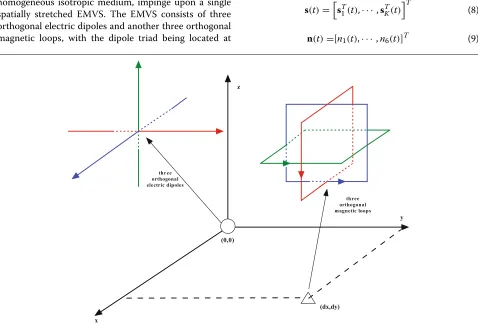
2 Mathematical data model and assumptions Assume that there are K uncorrelated monochromatic transverse electromagnetic signals, parameterized by {θ1,φ1},· · ·, {θK,φK}, after having traveled through a homogeneous isotropic medium, impinge upon a single spatially stretched EMVS. The EMVS consists of three orthogonal electric dipoles and another three orthogonal magnetic loops, with the dipole triad being located at

(0, 0)and the loop triad being located at(dx,dy), as shown in Fig.1. The parameter 0≤θk < πdenotes the elevation angle of thekth signal, and 0 ≤ φk < 2π represents the azimuth angle. The 6 × 1 data vector measured by the EMVS at time instanttcan be expressed as [2]

z(t)=

K

k=1

Aksk(t)+n(t)=As(t)+n(t) (1)

where

Ak =A(θk,φk)=[a1,k,a2,k]=

v1,k v2,k

qkv2,k −qkv1,k

(2)

v1,k=[cosθkcosφk, cosθksinφk,−sinθk]T (3)

v2,k =[−sinφk, cosφk, 0]T (4)

qk=ej2π/λ(dxsinθkcosφk+dysinθksinφk) (5)

A=[A1,· · ·,AK] (6)

sk(t) = [sk,1(t),sk,2(t)]T

= βk,1ej(ωk,1t+ψk,1),βk,2ej(ωk,2t+ψk,2) T

(7)

s(t)=sT₁(t),· · ·,sT_K(t)T (8)

n(t)=[n1(t),· · ·,n6(t)]T (9)

In the above equations,

• Akis the6 × 2EMVS response of thek th

electromagnetic signal.

• Ais the6×2KEMVS steering matrix.

• sk(t)is a2 × 1vector, representing the two entries

of thek th transmitted signal.

• In (7),βk,i,ωk,iandψk,i,i,=1, 2, respectively,

represent the energy, frequency, and the uniformly distributed random phase of thei th entry of the k th signal.

• n(t)is the6 × 1noise vector.

Note that the rank of the covariance matrix of thekth signalRsk = E

sk(t)sHk(t)

is related to the polarization state of thekth signal [24,25]. For the case of an incom-pletely polarized (IP) signal, the covariance matrixRsk is of rank-2, whereas for the case of completely polarized (CP) signal,Rsk becomes rank deficient. In other words, the IP signal possesses two spatial degrees of freedom, whereas the CP signal has only one. Referring back to (7), ifωk,1 = ωk,2, then the signal is IP, and its polarization varies with time. On the other hand, ifωk,1 = ωk,2 =ωk, then the signal is CP, and it has constant polarization. For the CP signal,sk(t)can be expressed as [25]

sk(t)=gksk(t)=

sinγkejηk cosγk

sk(t) (10)

whereγk andηk are polarization parameters referred to as the auxiliary polarization angle and polarization phase difference, respectively, andsk(t)=βkej(ωkt+ψk)is thekth transmitted signal. Thus, for the case ofKCP signals, the data vector in (1) reduces to the one used in [3].

The data vector model in (1) is only valid for ideal vector sensors. For practical vector sensors, the mutual coupling across the six vector sensor components is not negligible. In such a realistic situation, the signal received by a vec-tor sensor component is no longer related to the wavefield incident on that component only, but can be expressed as a linear combination of the wavefields incident onto all the six vector sensor components. To take the coupling effect into account, the data model in (1) needs to be modified by including a 6 × 6 matrix termM, referred to as the coupling matrix, which expresses the aforementioned lin-ear combination. Therefore, the data vector in the pres-ence of mutual coupling can be written as

z(t)=MAs(t)+n(t) (11)

The mutual coupling matrixMmay contain 36 distinct parameters. Thus, a full coupling matrix model usually requires too many parameters to be estimated. There-fore, a simplified version of M is required. If a priori knowledge on the mutual coupling matrix is available, then its exploitation can be useful in reducing the number

of parameters to be estimated, thus, making the estima-tion procedure simpler. In light of this consideraestima-tion, we assume that the displacement between the dipole triad and the loop triad is large enough so that the mutual cou-pling coefficients between the dipole triad and the loop triad are zero. This hypothesis can be justified by the fact that the coupling decreases quite rapidly with distance [11]. Furthermore, since the components in the dipole triad and loop triad are orthogonal to one another, all the components of a vector sensor would experience the same coupling effect. Therefore, the mutual coupling matrixM

can be formulated as

M = I2⊗C = I2 ⊗ ⎡

⎣cc12 cc21 cc22

c2 c2 c1 ⎤

⎦ (12)

where c1 andc2represent the self and mutual coupling coefficients, respectively.

With a total ofNsnapshots taken at the distinct instants {nT : n = 1,· · ·,N}, the problem is to determine the DOA’s{(θk,φk),k = 1,· · ·,K}of theKsignals and the coupling matrix C from these snapshots. The following assumptions are made:

1. The parameters(θ1,φ1),· · ·,(θK,φK)are pairwise

distinct.

2. The value ofK is known or correctly estimated. 3. The coupling coefficientsc1 = c2so that the

coupling matrixCis non-singular.

4. The impinging signals are IP and are uncorrelated with one another. This implies that the frequencies ω1,1=ω1,2= · · · =ωK,1=ωK,2.

5. The noise is zero-mean, complex Gaussian, and is statistically independent of all the signals.

3 Joint angle and mutual coupling matrix estimation

3.1 Temporal smoothing

The authors in [4] have found that the maximum number of arbitrary electromagnetic sources uniquely identifiable by one vector sensor is two. That is, the data matrix in (11) is rank deficient if the number of incoming signals is greater than two. In this subsection, we will apply the temporal smoothing technique [26] to deal with this rank deficiency problem. We will also show that under certain conditions, the temporal smoothing technique can restore the rank of the data matrix.

Define a6×Ndata matrix Z=[z(T),· · ·,z(NT)],

where z(T),z(2T),· · ·,z(NT)are theNsnapshots

sampled at time instants T, 2T,· · ·,NT,

Z1=[z(T),· · ·,z((N−P+1)T)] (13)

is a diagonal matrix that is only dependent on the time delay and the frequencies of the signals, and

S=[s(T),· · ·,s((N−P+1)T)]T (16)

is a(N−P+1)×2Ksignal matrix. Then, forp = 1,· · ·,P, we will havePdifferent data sets{Z1,· · ·,ZP}. Note that thesePdata sets differ from one another in view of the fact the the matricespdiffer from one set to another. Next, the 6P×(N−P+1)temporally smoothed data matrix is temporally smoothed data matrixZTSis of full rank2K .

ProofThe matrix ZTS can be expressed in a column-wise Kronecker matrix product form as

ZTS = (MA)ST (18)

Since all the signals are assumed to be IP and have distinct frequencies, the Vandermonde matrixSis of full column

rank 2K if and only if(N − P + 1) ≥ 2K. Next, by results in [27], we have

rank(MA) ≤ min{2K, rank()·rank(MA)}

and a sufficient condition for equality is to haveand/or

MAtall and full rank. Then, ifP ≥ 2K, the Vandermonde rank. This concludes the proof.

Theorem1establishes sufficient but not necessary con-ditions for constructing temporally smoothed matrices to resolveKIP monochromatic signals with a single-vector sensor. Specially, on the basis of Theorem 1, an infinite number of uncorrelated signals with distinct frequencies may potentially be resolved asNapproaches infinity.

3.2 Angle and mutual coupling matrix estimation In this subsection, we propose an ESPRIT-based algo-rithm to estimate the angles and the coupling matrix from the data matrix ZTS. For analytical purposes, we con-sider the ideal noiseless case. Let Es be the 6P × 2K signal-subspace eigenvector matrix, whose columns are the 6P × 1 signal-subspace eigenvectors associated with the 2Klargest eigenvalues ofZTSZHTS. Using the basic idea of ESPRIT [28], we have

Es = (MA)T=BT (20)

whereB = MA, andTis a unique 2K × 2K non-singular matrix. Next, define the following two selection matrices

J1=[I6P−6,0(6P−6)×6] ,J2=[0(6P−6)×6,I6P−6] (21)

and letB1 = J1BandB2 = J2B. The shift invariance structure inBindicates that

Note that the matrixB1has the form

It should be pointed out that the estimatedQˆ would suffer the unknown scaling ambiguities of the columns. That is, the columns of the estimatedQˆ in fact satisfy

q2k−1 = α1,kCv1,k, q2k = α2,kCv2,k (28)

¯

q2k−1 = ¯α1,kCv2,k, q¯2k = ¯α2,kCv1,k (29)

whereq2k−1,q2kandq¯2k−1,q¯2k,k = 1,· · ·,K, respec-tively, denote the top three and bottom three rows of the (2k − 1)th and(2k)th columns of Qˆ, αi,j andα¯i,j,

i = 1, 2,j = 1,· · ·,K represent the unknown scalars. Note that sinceqk = 1,αi,jis in general unequal toα¯i,j.

The scaling ambiguities can be easily eliminated in the proposed method. Usingq2k = α2,kCv2,k, we can form first, second, and third entries of q2k. Solving these three equations yields the azimuth angle and coupling coefficient estimates:

With the estimation of the coupling coefficientcˆ, we can construct an estimate of the mutual coupling matrixCˆ as

ˆ

It is easy to see that the matrix product CCˆ becomes a scaled identity matrix. This means that the mutual coupling coefficients, which constitute the non-diagonal

elements ofC, are completely eliminated. With the esti-mation ofφˆk andˆc, usingq¯2k = ¯α2,kCv1,k, we can form

Solving these three equations leads to the elevation angle estimates

Note that the estimation of θˆk andφˆk are automatically paired without any additional processing.

In practice, apart from the scaling ambiguities, the esti-matedQˆ may also suffer from some permutation ambigu-ities. In this case,q2kmay not be the estimate ofα2,kCv2,k. Thus, the estimation ofφˆk andcˆobtained by using (33) and (34) from q2k may be erroneous. These may fur-ther result in the erroneous estimation ofθˆk. Unlike the scaling ambiguities, the permutation ambiguities are not resolvable. Here, we provide a solution to deal with this permutation ambiguity problem as follows: first, for all

k = 1,· · ·, 2K, obtain a set of 2K different azimuth angle estimates fromqk. Each of these 2K azimuth angle estimates is then used to produce its own coupling coeffi-cient and elevation angle estimates. Thus, thekth azimuth angle, elevation angle, and coupling coefficient estimates are automatically matched. We know that only a set of

K estimates are true estimates. Theoretically, theKtrue coupling coefficient estimates are identical, while the K

erroneous coupling coefficient estimates are, in general, distinct from one another and from theKtrue estimates. Therefore, we can take homogeneity in coupling coeffi-cient estimates as a criterion for determining the true estimates of the angles and coupling coefficients, i.e., we take a set of K angle estimates associated with K iden-tical coupling coefficient estimates as the true estimates. Without loss of generality, let us assume that the firstK

3.3 Remarks

In the presence of noise, the estimation procedures in Section 3.2becomes approximate. Specially, with noise, the set ofKcoupling coefficient estimates are in general different. Nevertheless, we can search for a set ofK cou-pling coefficient estimates with “most similar values” as the “identical” estimates.

Also note that the vector cross product estimator has been widely used for direction finding with a single-vector sensor [2, 3, 7]. However, this estimator cannot be exploited directly in the presence of mutual coupling among the vector sensor components. Obviously, with the estimation ofcˆ, the vector sensor can be calibrated by using the calibration matrix defined as Mˆ = I2⊗

ˆ

C. Therefore, the vector cross product estimator can be applied to the calibrated data matrix MZˆ to extract the angle estimates of the incoming signals. Although the pro-posed method is designed for vector sensors with mutual coupling, it can also be applied to ideal vector sensors, where the measurement of each component is indepen-dent of the others.

The proposed method shares all the advantages indi-cated in [3]. For example, it offers automatically paired azimuth and elevation angle estimates, does not restrict T to be constricted by the Nyquist sampling rate, does not need the signal frequencies to be known a priori, and suffers no frequency-DOA ambiguity. It should be noted that the method in [3] assumes CP signals, whereas the proposed method assumes IP ones.

Lastly, it should be pointed out that the application of ESPRIT technique for vector sensor mutual coupling cali-bration has been studied in works [22] and [23]. However, the differences between these two works and the present work are that (1) the former requires a coupling-free aux-iliary vector sensor and design of a reference signal, while the latter does not, (2) the former does not apply the tem-porally smoothing technique to improve the identifiability limit of a vector sensor, and (3) the former assumes the incoming signals are completely polarized, while the latter considers the incompletely polarized signals.

4 Cramér-Rao bound

This section derives the CRB for the problem considered above, under the assumptions made in Section 2. Fur-ther, the following assumptions are added: (i) we assume

c1 = 1 andc2 = c = 1 due to the fact that the vector sensor can be calibrated with the estimation ofc = c2/c1. (ii) Since the spatial phase factorqk between the dipole triad and loop triad is considered as a scalar constant in the proposed method, we assumeqk = 1,k = 1,· · ·,K for convenience. (iii) The energies, frequencies and initial phases of the signals are presumed as known constants. (iv) The 6 × 6 noise covariance matrixRn is presumed as unknown, deterministic, and diagonal with all diagonal

elements equal toσ2_{. Hence, the observation data satisfies} the following model:

matrix(FIM) is given by

J(θ) = 2 a block matrix form as

J(θ)=

where all the blocks are of size 2×2. Using the fact that for largeN, _N1N_n=1si(nT)s∗_j(nT)=δij, whereδijdenotes the Dirac delta,J(θ)would asymptotically have the form

where

Finally, computing the inverse of the FIM, we obtain the following closed-form expression for the CRB:

CRB(c)= σ

5 Simulation results and discussion

5.1 Simulation results

In this section, we provide simulation results to illustrate the performance of the proposed ESPRIT-based method. In all the simulations, the vector sensor is assumed to be spatially collocated with the mutual coupling model defined in (12). The mutual coupling coefficient used is

c=0.1e−jπ/4. The additive noise is assumed to be spatial white complex Gaussian, and the SNR is defined relative to each signal. The result in each of the examples below is obtained from 500 independent Monte-Carlo trials. For comparison purposes, three different methods are consid-ered. The first method is to apply the vector cross product estimator to the measured data directly. This method is hereafter referred to as “VCP Estimator without calibra-tion.” The second method is based on the condition that the mutual coupling coefficient is known a priori, and the vector cross product estimator is applied to the per-fectly calibrated data. This method is referred to as “VCP Estimator perfect calibration.” The third method is the auxiliary sensor calibration method presented in [22]. The performance metric used is the root mean squared error (RMSE) of the two signals.

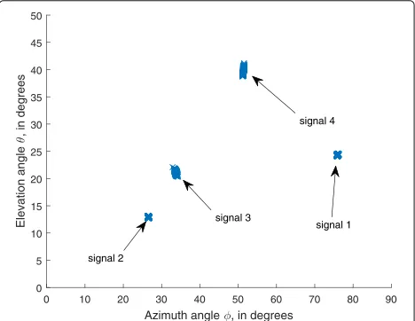
In the first example, we present the scatter diagram of the azimuth-elevation angle estimates of four source signals in Fig. 2 to show the effectiveness of the tem-poral smoothing technique. The angles of signals are set as (θ1,· · ·,θ4) = (24.35°, 12.92°, 21.13°, 39.82°) and (φ1,· · ·,φ4)=(75.96°, 26.57°, 33.69°, 51.34°). The SNR is assumed to be 25 dB andN = 15 data samples are used.

P = 8 is used for performing the temporal smoothing processing. From the figure, we can see that the proposed

Fig. 2Angle estimation result for four source signals. The angles of signals are set as:(θ1,· · ·,θ4)=(24.35°, 12.92°, 21.13°, 39.82°) and

(φ1,· · ·,φ4)=(75.96°, 26.57°, 33.69°, 51.34°). Five hundred

method successfully resolves the four signals, as stated in Theorem1:N ≥4K−1.

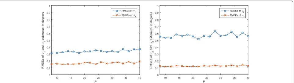
In the second example, we study the performance of the proposed method with different temporal smoothing dimensionP. Two equal-power narrowband uncorrelated monochromatic IP signals with randomly chosen digital frequencies impinge upon the vector sensor with angles: θ1 = 21.13°,φ1 = 33.69° andθ2 = 39.82°,φ2 = 51.34°. The number of snapshots and SNR used are, respectively,

N = 200 and SNR = 25 dB. The RMSEs of angle esti-mates as a function of the valueP, varying from 8 to 40, are shown in Fig.3. We see from the figure that the estima-tion errors remain almost unchanged with the increasing of valueP.

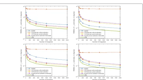
In the third example, we compare the performance of the proposed method with the VCP Estimator without calibration, VCP Estimator perfect calibration, and auxil-iary sensor calibration method. The simulation conditions are similar to those in the second example, except that the SNR is varying from 0 to 40 dB in steps of 5 dB. The RMSEs of angle estimates are shown in Fig.4, where the CRBs are also plotted for comparison. We see from the figure that the proposed method has a performance sig-nificantly superior to that of the VCP Estimator without calibration. For azimuth angle estimation, the proposed method outperforms the VCP Estimator perfect calibra-tion and auxiliary sensor calibracalibra-tion method at all SNRs. For elevation angle estimation, the RMSEs of the pro-posed method are slightly greater than those of the VCP Estimator perfect calibration and auxiliary sensor cali-bration method. This phenomenon can be explained as follows. Referring back to (33), (34), and (39), the pro-posed method obtain the estimates of azimuth angles, coupling coefficients and elevation angles in a successive way, and the estimation of the elevation angles is based on the previous estimations of the azimuth angles and the mutual coefficient. Consequently, the errors in the

azimuth angle and coupling coefficient estimates will pro-duce additional errors in the elevation angle estimates. Note that, with the estimation of coupling coefficient, the estimation performance for elevation angle can be further improved by statistically optimal algorithms such as maxi-mum likelihood algorithm and subspace fitting algorithm. Incidentally, since the estimate errors are a bit bigger than CRB, the proposed method might be biased.

In the fourth example, we assess the performance of the proposed method versus the number of snapshots. The simulation conditions are similar to those in the sec-ond example, except that the SNR is set at 20 dB and the number of snapshots is varied from N = 20 to N =

2000. The RMSEs of the angle estimates are plotted in Fig. 5, and compared with those of the VCP Estimator without calibration, VCP Estimator perfect calibration, auxiliary sensor calibration method, and the CRBs. We see from Fig. 5 that the results are similar to those of the first example. The RMSEs of the proposed method decrease monotonically with the number of snapshots. Moveover, for azimuth angle estimation, the RMSEs of the proposed method are lower than those of the VCP Esti-mator perfect calibration and auxiliary sensor calibration method.

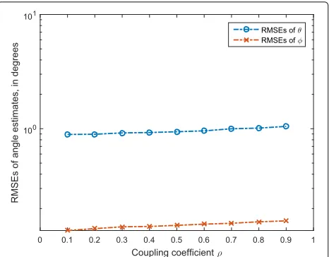
In the last example, we investigate the RMSEs of angle estimates for the proposed method against the coupling level, which is represented by coupling coefficient c =

ρejπ/4, varying low (ρ = 0.1) to high (ρ = 0.9). One IP signal withθ =21.13°,φ =33.69°, and randomly chosen digital frequencies impinges upon the sensor. The num-ber of snapshots and SNR used are, respectively,N=200 and SNR = 25 dB. The RMSEs of angle estimates as a function of the value ρ are shown in Fig. 6. We see from the figure that the proposed method can handle both low and high coupling levels, since the estimation errors remain almost constant with the increasing of coupling coefficientρ.

Fig. 3RMSEs of angle estimates againstP. Two uncorrelated signals withθ1=21.13°,φ1=33.69° andθ2=39.82°,φ2=51.34° impinge upon a

Fig. 4RMSEs of angle estimates against SNR. Two uncorrelated signals with_θ1=21.13°,φ1=33.69° andθ2=39.82°,φ2=51.34° impinge upon a

single-vector sensor. Five hundred independent experiments are conducted

Fig. 5RMSEs of angle estimates against snapshots. Two uncorrelated signals withθ1=21.13°,φ1=33.69° andθ2=39.82°,φ2=51.34° impinge

Fig. 6RMSEs of_θand_φestimates versus coupling coefficient_ρ. Five hundred independent experiments are conducted

5.2 Discussion

The proposed method is valid only for the case ofK ≥2. If there is only one incoming signal, this method can-not be used. In this case, the temporal smoothing process is not necessary, and a method for determining the true estimates is formulated as follows: let En be the 6 × 4 noise-subspace eigenvector matrix whose four columns are the 6×1 noise-subspace eigenvectors associated with four smallest eigenvalues ofZZH. For the two sets of esti-mates

, we may determine as to which one is the true one by first constructing the matri-cesI2⊗ ˆC1Aˆ1andI2⊗ ˆC2Aˆ2, and then taking

ˆ c1,θ1ˆ,φ1ˆ

to be the true estimates if $$

otherwise, where||·||denotes the Frobenius norm.

6 Conclusions

The present paper has considered, for the first time, the direction finding using a single-vector sensor in the presence of mutual coupling. The temporal smoothing technique has been applied to improve the identifiability limit of a single vector. In particular, sufficient conditions for constructing temporally smoothed matrices to resolve

K > 2 incompletely polarized (IP) monochromatic sig-nals with a single vector sensor have been established. An efficient ESPRIT-based method, which does not require any calibration sources or iterative operations, has been developed to jointly estimate the azimuth-elevation angles and the mutual coupling coefficients. The CRB for the considered problem has also been derived. Simulation results have been presented showing the superiorities of the proposed method.

Acknowledgements

The authors would like to thank the anonymous reviewers for their valuable comments and suggestions that helped improve the quality of this manuscript.

Funding

This work was supported by the National Natural Science Foundation of China (no. 61771302) and Shanghai Association of Science and Technology (no. 16511103004)

Availability of data and materials

The datasets generated and/or analyzed during the current study are not publicly available but are available from the corresponding author on reasonable request.

Authors’ contributions

All authors contributed extensively to the study presented in this manuscript. TS presented the main idea, carried out the simulation, interpreted the results, and wrote the paper. KW and JH conceived of the experiments. They also provided many valuable suggestions to this study. ZL supervised the main idea and edited the manuscript. All authors read and approved the final manuscript.

Authors’ information

Ting Shu received the B.Sc. and M.Sc. degrees from Nanjing University of Science and Technology, Nanjing, China, in 2004 and 2006, respectively, both in electrical engineering. He received the Ph.d degrees in electrical engineering from Shanghai Jiao Tong University, Shanghai, China, in 2010. From 2010 to 2011, he worked as the system engineer in the Wireless Department of Huawei Technologies, Co., Ltd., responsible for the HSDPA baseband system design for the UMTS evolution. He joins SJTU in July, 2011. He is currently an assistant professor in electrical engineering at Shanghai Jiao Tong University. His current research interests include the hardware-in-loop simulation of radar and EW systems, R&D of radar realtime signal processing, and adaptive array for phased array radar system. (Email: [email protected]) Kun Wang received the B.S. and Ph.D. degrees from Nanjing University of Science and Technology (NJUST), Nanjing, Jiangsu, China, in 2008 and 2017, respectively, both in electrical engineering. He is now a postdoctoral fellow with the Department of Electrical Engineering, Shanghai Jiaotong University, Shanghai, China. His research interests include sensor-array signal processing, statistical signal processing and their applications to sensors/radar networking. Jin He received his B.S. degree in information engineering from Tongji University, Shanghai, China in 2001 and his M.S. and Ph.D. degrees in electrical engineering from Nanjing University of Science and Technology (NJUST), Nanjing, Jiangsu, China in 2004 and 2007, respectively. From 2007 to 2009 he was a postdoctoral fellow with the Department of Electrical Engineering, NJUST, where he was the program director and was responsible for the China Postdoctoral Science Projects. From 2009 to 2011 he was a postdoctoral fellow with the Department of Electrical and Computer Engineering, Concordia University, Montreal, Quebec, Canada. From 2012 to 2015 he was a research engineer with the Shanghai Aerospace Electronic Technology Institute, Shanghai, China. He is now with the Shanghai Key Laboratory of Intelligent Sensing and Recognition, Department of Electronic Engineering, Shanghai Jiaotong University, Shanghai, China. Also he has served as a peer-reviewer for various IEEE/IET research journals since 2007. His research interests include array signal processing, statistical signal processing, non-Gaussian signal processing, and their applications.

Zhong Liu received the B.S. degree from Anhui University, Hefei, Anhui, China, in 1983 and the M.S. and Ph.D. degrees from University of Electronic Science and Technology of China, Chengdu, Sichuan, China, in 1985 and 1988, all in electrical engineering. He was a Postdoctoral Fellow at Kyoto University, Kyoto, Japan, from1991 to 1993 and a visiting scholar at the Chinese University of HongKong, Hong Kong, from 1997 to 1998. Currently, he is a Professor in the Department of Electronic Engineering, Nanjing University of Science and Technology. His research interests include chaos and information dynamics, signal processing, radar and communication techniques.

Competing interests

The authors declare that they have no competing interests.

Publisher’s Note

Author details

1_{Shanghai Key Laboratory of Intelligent Sensing and Recognition, Department}

of Electronic Engineering, Shanghai Jiaotong University, Shanghai 200240, People’s Republic of China.2_{Department of Electronic Engineering, Nanjing}

University of Science and Technology, Nanjing 210094, People’s Republic of China.

Received: 28 July 2017 Accepted: 12 February 2018

References

1. J Li, Direction and polarization estimation using arrays with small loops and short dipoles. IEEE Trans. Antennas Propag.41, 379–387 (1993) 2. A Nehorai, E Paldi, Vector-sensor array processing for electromagnetic

source localization. IEEE Trans. Signal Process.42, 376–398 (1994) 3. KT Wong, MD Zoltowski, Uni-vector-sensor ESPRIT for multisource

azimuth, elevation, and polarization estimation. IEEE Trans. Antennas Propag.45, 1467–1474 (1997)

4. KC Tan, KC Ho, A Nehorai, Linear independence of steering vectors of an electromagnetic vector sensor. IEEE Trans. Signal Process.44, 3099–3107 (1996)

5. J Zhang, CC Ko, A Nehorai, Separation and tracking of multiple broadband sources with one electromagnetic vector sensor. IEEE Trans. Aerosp. Electron. Syst.38, 1109–1116 (2002)

6. A Nehorai, P Tichavsky, Cross-product algorithms for source tracking using an EM vector sensor. IEEE Trans. Signal Process.47, 2863–2867 (1999)

7. KT Wong, X Yuan, Vector cross-product direction-finding with an electromagnetic vector-sensor of six orthogonally oriented but spatially non-collocating dipoles/loops. IEEE Trans. Signal Process.59, 160–171 (2011)

8. X Yuan, Estimating the DOA and the polarization of a polynomial-phase signal using a single polarized vector-sensor. IEEE Trans. Signal Process.

60, 1270–1282 (2012)

9. BC Ng, CMS See, Sensor array calibration using a maximum likelihood approach. IEEE Trans. Antennas Propag.44, 827–835 (1996) 10. F Sellone, A Serra, A novel online mutual coupling compensation

algorithm for uniform and linear arrays. IEEE Trans. Signal Process.55, 560–573 (2007)

11. Z Ye, J Dai, X Xu, X Wu, DOA estimation for uniform linear array with mutual coupling. IEEE Trans. Aerosp. Electron. Syst.45, 280–288 (2009) 12. J Dai, Z Ye, Spatial smoothing for DOA estimation of coherent signals in

the presence of unknown mutual coupling. IET Signal Process.5, 418–425 (2011)

13. J Dai, W Xu, D Zhao, Real-valued DOA estimation for uniform linear array with unknown mutual coupling. Signal Process.92, 2056–2065 (2012) 14. W Wang, S Ren, Y Ding, H Wang, An efficient algorithm for direction

finding against unknown mutual coupling. Sensors.14, 4–20077 (2006) 15. B Liao, S Chan, A cumulant-based approach for direction finding in the

presence of mutual coupling. Signal Process.104, 197–202 (2014) 16. J Dai, X Bao, N Hu, C Chang, W Xu, A Recursive RARE Algorithm for DOA

Estimation With Unknown Mutual Coupling. IEEE Antennas Wirel. Propag. Lett.13, 1593–1596 (2014)

17. M Lin, L Yang, Blind calibration and DOA estimation with uniform circular arrays in the presence of mutual coupling. IEEE Antennas Wirel. Propag. Lett.5, 315–318 (2006)

18. J Dai, D Zhao, X Ji, A sparse representation method for DOA estimation with unknown mutual coupling. IEEE Antennas Wirel. Propag. Lett.11, 1210–1213 (2012)

19. N Hu, Z Ye, X Xu, M Bao, DOA estimation for sparse array via sparse signal reconstruction. IEEE Trans. Aerosp. Electron. Syst.49, 760–773 (2013) 20. J Dai, N Hu, W Xu, C Chang, Sparse Bayesian learning for DOA estimation

with mutual coupling. Sensors.15, 7–26280 (2626)

21. Y Wang, M Trinkle, BW-H Ng, DOA estimation under unknown mutual voupling and multipath with improved effective array aperture. Sensors.

15, 30856–30869 (2015)

22. G Wang, H Tao, J Su, X Guo, C Zeng, L Wang, inAntennas, Propagation & EM Theory (ISAPE) 2012 10th International Symposium on. Mutual coupling calibration for electromagnetic vector sensor array (IEEE, Xian, 2012), pp. 261–264

23. L Wang, G Wang, C Zeng, Mutual coupling calibration for electromagnetic vector sensor. Prog. Electromagn. Res. B.52, 347–362 (2013)

24. KC Ho, KC Tan, A Nehorai, Estimating directions of arrival of completely and incompletely polarized signals with electromagnetic vector sensors. IEEE Trans. Signal Process.47, 2845–2852 (1999)

25. K Wang, J He, T Shu, Z Liu, Localization of mixed completely and partially polarized signals with crossed-dipole sensor arrays. Sensors.15, 31859–31868 (2015)

26. AN Lemma, AJ van der Veen, EF Deprettere, Analysis of joint

angle-frequency estimation Using ESPRIT. IEEE Trans. Signal Process.51, 1264–1283 (2003)

27. MC Vanderveen, AJ van der Veen, A Paulraj, Estimation of multipath parameters in wireless communications. IEEE Trans. Signal Process.46, 682–690 (1998)