Feature Subset Selection in
Conditional Random Fields for Named Entity Recognition
Roman Klinger and Christoph M. Friedrich
Department of Bioinformatics
Fraunhofer Institute for Algorithms and Scientific Computing (SCAI)
53754 Sankt Augustin, Germany
{
roman.klinger,christoph.friedrich
}
@scai.fraunhofer.de
Abstract
In the application of Conditional Random Fields (CRF), a huge number of features is typically taken into ac-count. These models can deal with inter-dependent and correlated data with an enormous complexity. The application of feature subset selection is important to improve performance, speed and explainability. We present and compare filtering methods using infor-mation gain orχ2as well as an iterative approach for
pruning features with low weights.
The evaluation shows that with only 3 % of the orig-inal number of features a 60 % inference speed-up is possible. TheF1measure decreases only slightly.
1 Introduction
Feature selection is well established for many machine learn-ing methods, for instance for feed-forward neural networks [2] or decision trees [17]. The main advantages are an im-provement of prediction performance, faster training and prediction as well as a better understanding of the models [4]. Methods can be distinguished between filters not us-ing the learnus-ing algorithm and wrappers usus-ing the learnus-ing algorithm as a black box [8]. An overview of approaches for classification tasks is given by Liu and Motoda [11], more specifically for text classification by Yang and Peder-son [25].
Such feature selection methods are not well established for Conditional Random Fields [9], a Maximum Entropy-based method [1] for structured data. We propose methods coping with the demanding task of handling sequential data represented by a huge number of features. Reported num-bers are for instance 1,686,456 for a gene name tagger [5]. Due to this high complexity, training and inference times can explode. These high numbers of features are generated by automated methods, i. e., for every token in the train-ing set, features are generated. Then, all other tokens are tested for these features. This method is typically applied to determine the identity of words as well as for prefixes or suffixes of different length or for learning schemata of regular expression-like patterns [20].
Only a few approaches dealing with feature handling for CRFs are published. The work by McCallum [12] demon-strates a method for iteratively constructing feature con-junctions that would increase conditional log-likelihood if
added to the model. An analysis of different penalty terms for regularization is shown by Peng and McCallum [15]. Goodman [3] presented a related analysis of exponential priors for Maximum Entropy models. The very recent work of Vail et al. [23, 22] shows feature selection in Conditional Random Fields byL1-norm regularization in the robotics
domain, a work which is related to the selection in Maxi-mum Entropy models proposed by Koh et al. [7].
These methods incorporate the training procedure in the selection process. In contrast, we present different filter methods for feature selection to limit the complexity before starting the training. It is demonstrated how the sequential structure of text can be respected by filtering approaches originally developed for classification problems (especially in Section 3.1.2 and 3.1.3). These filter methods are com-pared to an iterative approach.
The paper is organized as follows. A short description of Conditional Random Fields is given in Section 2. We intro-duce different approaches for feature selection in Section 3, namely the adaption of classification methods to filter fea-tures and an iterative approach to remove feafea-tures with low weights. In Section 4, an evaluation of the feature selection methods is given. The results show a reduction of complex-ity leading to improved speed and better explainabilcomplex-ity.
2 Conditional Random Fields and
Sequential Data
Conditional Random Fields [9, 13] are a family of prob-abilistic, undirected graphical models for computing the probability P~λ(~y|~x) of a possible label sequence ~y = (y0, . . . , yn) given the input sequence~x = (x0, . . . , xn). In the context of Named Entity Recognition, this ob-servation sequence ~x corresponds to the tokenized text. The label sequence is encoded in a label alphabetL = {I-<entity>,O,B-<entity>}whereyi=Omeans thatxi is outside an entity,yi=B-<entity>means thatxiis the beginning andyi=I-<entity>means thatxiis inside an entity.
In general, a CRF is given by
P(~y|~x) = 1 Z(~x)
n Y
j=1
Ψj(~x, ~y) (1)
ϕ(xj) = 1 ϕ(xj) = 0 P
L` h1j(`) h0j(`) h(`)
L6=` ¯h1j(`) ¯h0j(`) ¯h(`)
P
h1
j h0j h
Table 1: The2×2contingency table.
where
¯
h(`) = X
l∈{1,...,|L|2}\`
h(l),
and¯h1
j(l)and¯h0j(l)analogous. This approach is applied to rank the featuresϕ(xj)for every transitionL`separately. It is referred to asInformation Gain One-Against-All (IG-OAA). The runtime isO(m|L|)and therefore less than Sim-ple IG.
3.1.3 χ2-Statistics
Another well-known and often incorporated ranking method areχ2-statistics[16]. The2×2contingency table is defined
for each featureϕ(xj)and each transitionL`compared to all other transitions (cf. Table 1). Theχ2-statistic is then
computed by
χ2(ϕ(x
j),Lj) = h1
j(`)·¯h0j(`)−h0j(`)·¯h1j(`) 2
·h h(`)·h(`)¯ ·h0
j·h1j (9) Similar toIG OAA, this is performed to rank the features ϕ(xj)for every transitionL`separately. Therefore, the run-time is alsoO(m|L|). We refer to this method asχ2OAA.
3.1.4 Random
The most simple method is arandomranking and selection of features. This is used as a baseline to evaluate the other measures presented in the previous sections.
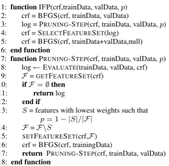
3.2 Iterative Feature Pruning
Training a CRF is commonly performed by the iterative algorithm L-BFGS to assign weightsλito all feature func-tionsfi ∈ F such thatL(T) is maximized (compare to Equation 4). Typically, many weights are close to0. The idea of Iterative Feature Pruning (IFP) is that feature func-tions with low absolute weight value have a low impact on the output sequence.
Based on this assumption, the algorithm (see pseudo code in Figure 1) starts with a fully optimized CRF using all features representing the training data (Line 2). The next step is the removal of features with lowest absolute value (3). The parameterp= 1− |S|
|F|specifies the percentage of
features to be removed in each iteration (13–15). Sis the set of remaining features after one iteration of IFP.
In each step, a retraining with L-BFGS is performed to allow an adaption of the model by adjusting the weights
1:functionIFP(crf,trainData, valData,p) 2: crf = BFGS(crf, trainData, valData)
3: log = PRUNING-STEP(crf, trainData, valData,p) 4: crf = SELECTFEATURESET(log)
5: crf = BFGS(crf, trainData+valData,null) 6:end function
7:functionPRUNING-STEP(crf, trainData, valData,p) 8: log←EVALUATE(trainData, valData, crf) 9: F=GETFEATURESET(crf)
10: ifF=∅then
11: returnlog
12: end if
13: S= features with lowest weights such that
p= 1− |S|/|F| 14: F=F\S
15: SETFEATURESET(crf,F) 16: crf = BFGS(crf, trainingData)
17: returnPRUNING-STEP(crf, trainData, valData) 18: end function
Figure 1: Iterative Feature Pruning Algorithm (starting with method IFP(·) in Line 1)
for the remaining features (16). After that, the pruning is repeated (17) until no features are left (11).
During this process, at each iteration of pruning, the current performance of the model is evaluated and stored (8). This information can be used to select the final feature set (Line 4, an heuristic is shown in Section 4.3) and to train a full model with the identified feature subset (Line 5).
To illustrate the process of IFP, it is shown exemplarily by means of extreme examples for one data set3in Figure 2. On the horizontal axis, all L-BFGS training iterations are shown consecutively with the intermediate pruning steps. The blue dotted line shows the decrease of the number of features, the red solid line theF1measure for the training data, the
green dashed line theF1measure for one validation data
set. Removing 40 % of the features in each step (p= 0.4) clearly depicts the process of removing and retraining of the model. Experiments4have shown that in general lower numbers of features can be achieved with comparableF1
measures if smaller values ofpare used. The drawback is the higher number of iterations needed. We focus on p= 0.1which leads to good results as shown in Section 4.
4 Results
In this section, the methods proposed in Section 3 are eval-uated on the data sets and configurations of the CRFs de-scribed in Section 4.1. The hypotheses to be analyzed are:
Selecting a reasonable subset of features: A1 Improves explainability of the CRF model,
A2 Improves training time and tagging time which is bene-ficial for developing as well as applying the model, A3 Improves performance inF1measure or does not
de-crease it dramatically.
Additionally, we assume that one method is superior to all others:
B One method outperforms the others.
Figure 2: Iterative Feature Pruning for CRF trained on CoNLL data with different percentages of features pruned in each iteration.
The evaluations in the following form the basis for the dis-cussion of these hypotheses in Section 4.4.
4.1 Data Sets used for Evaluation
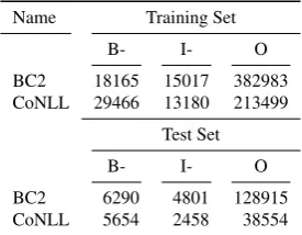
The results and evaluations are shown on the basis of two data sets with slightly different configurations of the CRF. Quantities of entities are given in Table 2.
The BioCreative 2 Gene Mention Task data (BC2) con-tains entities of the classGene/Proteinwith the specialty of acceptance of several boundaries for entities [24]. We incorporate the configuration of the CRF as described in a participating system using only the shortest possible annota-tion as exact true positive per entity [6, 21].
Name Training Set
B- I- O
BC2 18165 15017 382983 CoNLL 29466 13180 213499
Test Set
B- I- O
BC2 6290 4801 128915 CoNLL 5654 2458 38554
Table 2: Numbers of labels in data sets, the different entity classes are added in CoNLL.
CoNLL data set
BioCreative 2 data set
Figure 3: Comparison of the averageF1measure using 10-fold cross-validation. Used features are determined with methods de-scribed in Section 3. The transparent band shows the standard deviation. The arrows show a possible selection of the model features (g= 2·10−6,∆ = 0.02, cf. Section 4.3).
The CoNLL data [19] is an annotation of the Reuters corpus [10] containing the classesperson,organization, lo-cationsandmisc. We use an order-one CRF with offset conjunction combining features of one preceding and suc-ceeding token for each position in the text sequence. The feature set is fairly standard with Word-As-Class, prefix and suffix generation of length two, three and four as well as reg-ular expressions detecting capital letters, numbers, dashes and dots separately and as parts of tokens. The combination of the provided sets “train” and “testa” is used for training and “testb” for testing.
For evaluating the inference time on a larger set, a uni-form sample from the Medline5database of 10,000 entries is used additionally. Each one comprises titles, author names, and abstracts. The number of tokens is 958869 for BC2 and 960744 for CoNLL (additionally to BC2 tokenization, splitting on all dots is performed for CoNLL data).
4.2 Cross-Validation on the Training Sets
As a basis for parameter selection (presented in Section 4.3) and to evaluate the impact of feature selection, 10-fold cross
validation is performed on the training sets (Section 4.1). The results are shown in Figure 3. The curves depict the averageF1measure6 of the 10 partitions. The different
numbers of features are detected with different parameters specified for the respective selection method. The transpar-ent band around the line depicts the standard deviation for the according number of features.7The significance of the difference of the methods is tested regarding the area under the curves in Figure 3 via Welch’s t-test with a significance level ofα= 0.05.
Comparing the results on the two data sets, the methods lead to similar results whereas the differences are clearer on CoNLL data. All approaches outperform the random selection significantly. The approach ofχ2OAAis worse
than the conceptionally similarIG OAAand the more naive
Simple IGon BC2 data.
IG OAAoutperforms all other filtering approaches. As-suming the goal to reach the highest possibleF1measure, IFPleads to better results thanIG OAAon both data sets. Only if an extremely small number of features remains (fewer than about50),IG OAAleads to better results. The superiority ofIFPtoχ2OAAis significant (p= 0.02) on
the CoNLL data set.
4.3 Results on independent test sets
We need to find the parameter assignment to determine the feature subset in the final model. For the filter approaches, the parameter ispfilter. ForIFP, the meaningful number of features at which the pruning is stopped has to be detected. Based on the smoothed8values ofF1measure in 10-fold cross-validation (see Figure 3), we define two measures to automatically detect these parameters: The maximally ac-cepted loss inF1measure is denoted with∆, the threshold
for the gradient isg. The detection of the feature subset is performed via backward selection starting with high num-bers of features. The first position on the curve for which the gradient is smaller thangor theF1measure is smaller
than∆is selected. The valuesg= 2·10−6and∆ = 0.02
lead to the positions denoted by arrows in Figure 3. The results for these values are evaluated in the following. The advantage of backward selection to forward selection is that it may capture interacting features more easily [8].
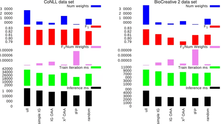
A model is built on the full training set applyingIFP
or filtering with the detected parameters. In Figure 4 the results on independent test sets mentioned in Section 4.1 are depicted. The smallest numbers of features are achieved by
IFPfollowed byIG OAA.
TheF1measures decrease up to the accepted∆ = 0.02
on BC2 data and to a lower amount for the CoNLL data. The best trade-off betweenF1measure and the number of
features (depicted in third bar chart) is always achieved by
IFPfollowed byIG OAA.
A smaller number of features should induce a faster model in training and inference. The time of evaluating 6Fβ=(1+β2)·precision·recall
β2·precision+recall , whereβ= 1
7In iterative feature pruning, different numbers of features can occur at the
same iteration of pruning. In that case, the closest detected number of features is used to compute average and standard deviation.
8Smoothing via computation of median in a running window.
P~λ(~y|~x)(compare to Equation 1) on all training examples is shown in the fourth bar charts. This computation is cru-cial for training durations as it has to be performed many times. These numbers correspond roughly to the number of features, the durations are smaller than for the original model. The ratio is not linear due to the necessary forward-backward algorithm calls (whose runtime is quadratic in the number of possible labels) and dynamic memory allocation times.
These numbers naturally lead to dramatically reduced training times. Training the full CoNLL model lasts5788 seconds,2397sfor BC2 respectively. With the feature set detected byIFP, these numbers reduce to2156sand670s. This improvement is not helpful in practice, as theIFP
procedure incorporates training the model. However, fil-tering viaIG OAAimproves overall training time as it is computationally inexpensive. It leads to5230sand1002s for training a model.9
Reducing the number of features also leads to a faster inference10: The fifth bar charts show durations for tagging 10000 sampled abstracts from Medline. Best results are achieved byIFP(CoNLL:10.52sinstead of17.56s, BC2: 2.42sinstead of4.56s), followed by the filtering methods which do not differ remarkably (IG OAA: CoNLL:14s, BC2: 2.65s).
Summarizing, a reduced training iteration time of76 % of original time evaluating P~λ(~y|~x) with a loss of only 1.7 %F1(absolute value) on the BC2 data is possible with IFP. The tagging time is reduced to53 %. On the CoNLL data, a loss of only0.57 %inF1occurs with savings of even
54 %of original computing time. Tagging time is reduced to60 %.
4.4 Discussion
Comparing the methods, the results are similar for the data sets: In 10-fold cross-validation, the random method is dominated by all other methods.Simple IGorχ2OAAare
second worst, depending on the data set. IFPis the best method, closely followed byIG OAA.
TheSimple IGlacks the representation of different tran-sitions in the features which is especially important for the CoNLL data with 4 entity classes of interest. No dictio-naries with members of these classes have been used in the presented setting, so all classes are memorized with automatically generated features, hence, a large number of different features is needed for the different transitions in the CRF.
The methodχ2OAAalways leads to worse results
com-pared toIG OAAon the 10-fold cross-validation although it is a systematically similar approach. The reason is pre-sumably the unbalancedness of the labels in the generated classification instances11which is taken into account in the
9The relation to the numbers of features and the iteration durations is not
linear as the needed numbers of training iterations differs.
10Measuring only the computation, not the time to read the data from hard
disk and to extract the features.
11Transitions of intermediate terms (like (O,O)) are for instance much
CoNLL data set BioCreative 2 data set
Figure 4: Results on independent test sets (Note the different scales for some of the histograms.)
information remainder (Equation 7 and 8) but not in χ2
(Equation 9).
IFPleads to better results thanIG OAAfor highF1
mea-sures. The reason is the limitation ofIG OAAto use the same number of features (but not the same set) for each transition (specified bypfilter). This does not hold forIFP as it only relies on the model structure itself. The drawback is the higher computational cost due to the incorporated L-BFGS optimization.
Therandommethod does not lead to good results, but it should be noted, that even this approach can remove 30 %–40 %without a dramatic decrease inF1measure. The
reason are unessential redundancies in the full feature set. Mainly all these results are reflected on the independent test sets.IFPorIG OAAhas the best trade-off betweenF1
measure and the number of features. Good inference speed-ups can be achieved with both methods, corresponding to the low numbers of features. However,IFPcannot be used to speed up training as it incorporates the training procedure itself. Hence,IG OAAis proposed for this instance. For re-ducing tagging time as well as for understanding the model,
IFPshould be used as it leads to the smallest numbers of features.
In Table 3, the percentages and numbers of remaining features accepting maximally0.01loss inF1measure are
depicted. Much more features can be ignored in the BC2 than in the CoNLL setting. This can be an indicator for the need for better generalizing features: as the classes have to be memorized by automatically generated features, less features can be eliminated. In BC2, features with better generalization characteristics are implemented.
We conclude the results with an investigation of the hypothe-ses:
A1 The explainability of models applying feature selection is improved by the lower complexity. The need for
Number of Features Data Set Original Remaining % CoNLL 269506 17377 6.45
BC 2 492611 11096 2.25
Table 3: Minimal numbers of original features needed to lose maximally 0.01 ofF1measure applying IFP.
many automatically generated features can be an indi-cator for a possible improvement by implementation of features with better generalization properties. Detected relevant features representing words or important pre-and suffixes help understpre-and the different entity classes of interest. The fact that noisy features are removed allows for an investigation of the remaining features which can be assumed as meaningful12
A2 Training and tagging time are decreased by the lower complexity of the CRF. To improve training time, the use of a filtering approach likeIG OAAis proposed as these methods are computationally inexpensive. To improve tagging time,IFPshould be used as it leads to the lowest numbers of features.
A3 A small decrease inF1 measure has to be accepted
for the benefit of a model with a considerable lower number of features.
B The recommendation for a method depends on the appli-cation: For improving training time, a filtering method should be used, preferablyIG OAAas it shows best re-sults. For improving tagging time, the computationally more expensiveIFPcan be applied.
12Lists of all features of the models are available online to demonstrate the