Article
PREDICT ARRIVAL TIME BY USING MACHINE LEARNING ALGORITHM TO PROMOTE UTILIZATION OF URBAN SMART BUS
Rafidah Md Noor1*, Ng Seong Yik1, Raenu Kolandaisamy2, Ismail Ahmedy1, Mohammad Asif Hossain1, Kok-Lim Alvin Yau3, Wahidah Md Shah4, Tarak Nandy1
1Faculty of Computer Science & Information Technology, University of Malaya, Kuala Lumpur, Malaysia
[email protected], [email protected], [email protected], [email protected], [email protected], [email protected]
2Faculty of Business & Information Science, UCSI University, Jalan Menara Garding, Kuala Lumpur, Malaysia
3Department of Computing and Information Systems, Sunway University, Selangor, Malaysia
4Faculty of Information and Communication Technology, Universiti Teknikal Malaysia Melaka, Melaka, Malaysia.
*Corresponding Authors
Abstract: The impact of the accurate estimated time of arrival (ETA) is often overlooked by bus operators. By providing accurate ETA to riders, it gives them the impression of bus services is efficient and reliable and this promotes higher ridership in the long run. This research project aims to predict bus arrival time by using the Support Vector Regression (SVR) model which is based on the same theory as the Support Vector Machine (SVM). Urban City Bus data covering part of the Petaling Jaya area (route name PJ03) is used in this research work. Features related to traffic such as travel duration, a distance of the road, weather and operation at peak or non-peak hour have been used as input in the training of the SVR model. By using kernel trick and specifying optimum parameters, all the features in higher dimensions are efficiently calculated and the SVR model achieves convergence. The model is evaluated with the test set of data split from the original dataset. The experimental result indicates the SVR model displays good prediction ability with its low average error on the prediction result. However, weather data has not been influential to the prediction model as the results of the model trained with and without weather data show a negligible difference.
Keywords: Support Vector Machine; Support Vector Regression; Machine learning; Prediction; Urban Smart Bus.
1. Introduction
It is inevitable that a developing country experiences urbanization and industrialization in different parts of the country, leading to the birth of cities. Urbanization and industrialization of cities have often led to a drastic change in the economy and environmental perspective [1]. Perhaps the most noticeable benefit from urbanization is improved economic growth, which helps to create more job opportunities and this further leads to an increase in population. However, urbanization and industrialization have brought not only benefits but drawbacks as well. For instance, from an environmental perspective, as more goods are sold and used within the city, more waste is being generated daily. Moreover, harmful materials that are not being disposed of properly can threaten our natural resources such as water sources. Other negative effects such as traffic jams, lack of parking space, congestions, noise pollution, and excessive carbon gas emissions are examples of consequences of urbanization in a city [2] as a result of increased travel demand by citizens. They need to rely on private vehicles or public transport to access different parts of the city. A well-connected transport system connecting different parts of the city is vital to enable all activities such as business to be performed daily to facilitate
growth. Without a good and functioning transport system, it’s nearly impossible for a city to continue its development, at least not consistently. However, many did not realize that mobility and transport system issues arise from urbanization can be detrimental to the development of a city if not resolved properly.
Private vehicle is clearly the preference of the citizens as the mode of transport in Malaysia. According to the Transport Minister of Malaysia Anthony Loke, the number of trips made by car daily will increase from 40 million to 131 million in the next 12 years and car ownership will increase by 1.4 times [3]. The trend of increasing private vehicle ownership is further supported by the statistics released by the Transport Ministry of Malaysia [4] showing an uptrend of the number of vehicles on the road in Kuala Lumpur from the year 2008 to the year 2015 (Figure 1). As a result of the ever-increasing number of vehicles on the road, congestions and road accidents happen more frequently. Asian Development Bank has suggested that road congestion could cost around 2% to 5% loss in gross domestic products (GDP) due to unnecessary time spent in traffic and higher transport cost [5]. There was a total of 72940 road accidents in Kuala Lumpur during the year 2017 (Figure 2). The World Bank stated that injuries and fatalities caused by road accidents resulted in the removal of the workforce hence reducing the productivity of a country [6]. In the longer-term, this can cost a country 7% to 22% of GDP over 24 years and this loss in GDP can be thought of as slowing down the development of a city or country.
The government recognized the issue of the transport system in Malaysia hence it has turned to public transport as a means to tackle the issue as public transport is a more sustainable alternative to travel compared to private vehicles. Public transport has been recommended as the primary mode of travel on numerous occasions [3, 7] to reduce road congestion issues and to reduce the number of road accidents, especially in Kuala Lumpur. However, it is not easy to change as there are different factors that may influent their choice of mode of transport. Take a public bus for example, travel time, frequency of bus service, safety and information about the service are among the factors that can potentially influence the public’s decision on choosing bus as the mode of transport [8]. Unfortunately, the transport system in Malaysia leaves a lot to be desired.
Figure 1. Number of Vehicles on the road in Kuala Lumpur from the year 2008 to 2015. (Ministry of Transport Malaysia, 2017)
Figure 2. The number of road accidents in Kuala Lumpur from the year 2008 to 2017. (Ministry of Transport, 2017)
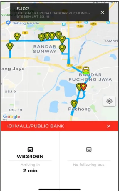
system, Selangor State Government has taken the initiative to partner up with Rapid Bus Sdn. Bhd. to introduce Smart Selangor Bus Service and PJ City Bus. Both services are fully funded by the state local government with the aim to promote the use of public transport, to ease the burden of people, and to reduce road congestion and pollution [10]. Selangor State Government has spent RM 78.6 million on Smart Selangor Bus Service to date [11]. Shah Alam, Kajang, Klang and Subang Jaya are among the areas covered by Smart Selangor Bus Service while PJ City Bus primarily covers the Petaling Jaya area. Both services start operating from 6.00 AM until 9.00 PM with a service frequency of 15 to 20 minutes on a working day and the buses are equipped with WiFi and are friendly to disabled people [12]. Selangor Intelligent Transport System (SITS) and PJ City Bus apps based on both Android and iOS platforms have been developed with the intention to increase the efficiency and reliability of the bus services. These mobile applications provide the public with information such as the nearest bus station, the estimated time of arrival (ETA) of the next bus and route information to help them to plan their journey more efficiently [13], [14]. Figure 3 displays the SITS interface while Figure 4 shows the interface of the PJ City Bus app.
Figure 3. The interface of SITS showing the bus stations and the ETA of a bus.
Figure 4. PJ City Bus app interface.
contributes to traffic congestion especially in the city area. SITS and PJ City Bus app do not consider weather conditions on their ETA calculation, as a result, accurate ETA is not achieved. This affects users in planning their journey if ETA provided is not accurate. The objective of this research is to attempt to develop a Support Vector Regression (SVR) model that can predict ETA of the bus at departure from a station to the next station by incorporating weather conditions.
The organization of the rest of this paper is as follows. Materials and methods are briefly introduced in Section 2. In Section 3, the results of the work are discussed. Section 4 discusses
the model performance. Finally, Section 5 gives the conclusion of the study.
2. Materials and Methods
Different models and approaches were proposed and conducted by researchers to predict the arrival time of the bus previously, but the majority of them found out that Support Vector Machine (SVM) and Artificial Neural Network (ANN) have outperformed other methods. Models proposed by previous researchers can be categorized into 4 groups [16] as presented in the rest of this section.
i. Historical Average Model
Historical Average Model is a relatively simple and resource un-intensive computational model that calculates the bus travel time by using average speed and distance. It uses historical data from previous bus journeys and assumes the traffic condition is the same for the upcoming journey [17]. There is a major drawback with this model --- it does not take other factors that can greatly affect the travel time into consideration. Most of the researches that used this model was proposed more than 5 years ago. [18] claimed that a few similar types of research have been conducted before the year 2010 that make use of this model.
ii. Regression Model
Having recognized that there are external factors or independent variables that can affect the prediction of bus arrival time, the regression model has been proposed. This method uses a mathematical function to calculate the output or dependent variable, in this case, the arrival time, with input or independent variables such as speed, road condition, weather and other possible variables [17]. The impact of all the independent variables are considered at once and each of the variables’ impact will affect the dependent variable. This addresses the issue where the Historical Average Model does not take other factors into account while predicting the bus arrival time. [17] has mentioned that distance, station number, dwell times, the number of boarding passengers and weather can be taken as independent variables in one of the previous studies to predict bus arrival time. One advantage of this model is that it can reveal the importance of the inputs.
iii. Kalman Filtering Model
worth noting that AVL is essential in Kalman Filtering Model in order to estimate the dynamic term in the model [20].
iv. Machine Learning Model
Machine learning is a technique for computers to learn how to do certain tasks without being explicitly programmed. It allows the machine to learn and make use of complex patterns of the processed data that cannot or difficult to be programmed by the human in a short period of time. There are more advanced machine learning methods such as ANN and SVM being proposed in recent years as machine learning has gained popularity. The recent advancement in computer processing power enables complex calculation and processing to be done significantly faster than in the past, and this has contributed to the rise in the popularity of machine learning techniques. Big companies such as Google and Amazon have utilized machine learning techniques to yield positive results and discovered potentials from a business perspective. The concept of ANN was proposed as early as the year 1943 by neurophysiologist Warren McCulloch and mathematician Walter Pitts [21]. The technique was designed to emulate how a human brain works. Many interesting neural network projects have been carried out ever since its introduction, for instance, the famous DeepMind by Google to play board games against professionals has gained huge success from it. ANN consists of a few layers, generally the input layer, hidden layer (there can be multiple hidden layers depending on the complexity of the problem) and output layer [22]. All the layers are interconnected, where the input layer consists of all the input variables, and all the input layers are connected to the hidden layers, and the hidden layer is connected to the output layer. Optimum weights of all the connections will be obtained through training and the correlation between input and output can be learned in the hidden layer. Unlike another method, ANN learns by example and is able to generalize what has been learned to solve a new problem without being explicitly programmed. This model can solve complex questions due to this nature; however, it is difficult to understand the underlying relationships within the model [17], [19]. Fan and Gurmu in [17] claimed that the non-linearity of ANN has contributed to the popularity gain of ANN in predicting bus arrival time. ANN is suitable to be used on the non-linear variables of the transportation system to predict bus travel time due to its ability to capture the non-linear relationship between them.
2.1Method
a) Support Vector Machine Overview
SVM was first developed by Vapnik based on statistical learning theory [23]. This algorithm has been applied in real-world situations, and it is regarded as one of the best classification systems for optical character recognition (OCR) or object recognition, while good performance has been achieved in regression and time series prediction problems. According to [24], SVM is an optimization algorithm by minimizing the structural risk rather than a greedy search. Concretely, SVM constructs a hyperplane that separates the input data or the training data into classes linearly. This hyperplane acts as the decision boundary, and this boundary has the maximum distance between the linearly separable classes [24], [25] [30]. The distance of a class to the boundary is often described as margin. If the classes are not linearly separable, the input data can be projected to a higher dimensional space using kernel function in order to obtain a hyperplane or decision boundary that separates the classes.
Among the strengths of SVM are: 1. Able to learn from a small sample size 2. Avoid local minimum and
3. Good generalization capability to unseen data.
Based on what has been mentioned in the previous section, SVM can construct a hyperplane that separates the input data. Considering the graphical example below in which the input data consists of two classes.
Figure 5. Different lines to separate the two classes.
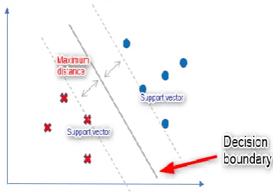
Figure 6. SVM finds a decision boundary that gives the maximum distance or margin. Support vectors are used to specify the decision boundary.
Both green and orange lines can be used to separate the two classes. In fact, there are so many possibilities for line placement to separate the classes. SVM is used to find the optimal line that separates these classes with maximum distance, or commonly known as margin, from the input data.
Based on Figure 5, if a new data falls at the side of the line near to the blue dot, then the new data is classified as a blue dot. On the other side, if a new data fall at the side of the line near to the red cross, then the new data is classified as a red cross. The decision boundary is determined by the support vectors, which are the input vectors that touch the boundary of the margin (dotted line in the above figure). Concretely, the decision boundary trained from the training data is used to classify new data.
Another example below where point A is far away from the decision boundary, while B is a point close to the decision boundary. In this case, point A is confidently classified as a blue dot while the confidence for B classified as a blue dot is not as high, and a slight change of the decision boundary can change the prediction result. The ideal situation is that all future predictions can be in high confidence.
Let’s portray the ideas of the examples above in equations. There is an input vector xi, where i
= 1 to n represents the number of features, then there are weight vectors wi that represents the
linear combination to predict the value of y or the binary class labels, and lastly b for intercept. For y, instead of the commonly used y ϵ {0,1} in logistic regression, SVM uses y ϵ {-1,1} as binary class labels. The functional margin of (w,b) with respect to training example (xi, yi) can be used to check on the confidence of the prediction:
ϒ(i) = y(i)(wT x + b) (1)
The larger the functional margin, the higher the confidence of the prediction is. Based on the functional margin equation, if y(i) is 1, in order for functional margin to be large, (wT x + b)
needs to be a large positive number. On the other hand, if y(i) is -1, (wT x + b) needs to be a
large negative number. Note that, for prediction to be correct, y(i)(wT x + b) must be larger than
0:
y(i)(wT x + b) > 0 (2)
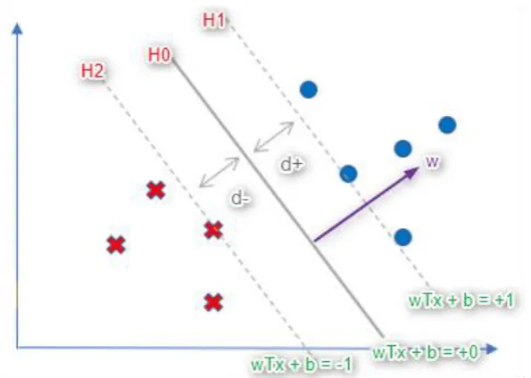
With this in mind, we can deduce that H1 and H2 are:
H1: (wT x + b) = +1 (3)
H2: (wT x + b) = -1 (4)
While d is the Euclidean distance:
d+: distance from the positive class, i.e. from H0 (decision boundary) to H1 (positive boundary line)
d-: distance from negative class, i.e. from H0 to H2 (negative boundary line).
Figure 8. The hyperplanes H and distance d. The point that touches the line H1 and H2 are the support vectors. W is orthogonal to the decision boundary.
Once again, the idea of SVM is to find the decision boundary with a maximum distance between the boundary and classes, and this requires the magnitude to be taken into consideration. It can be impossible to calculate the distance without the magnitude. Geometric margin is the Euclidean distance, d between the data point and the decision boundary, and this is obtained by normalizing the functional margin with magnitude ||w||.
ϒ𝑖 = 𝑦𝑖 (𝑤𝑇 𝑥 + 𝑏)
||w|| (5)
The constraint has been put on the size of the w by doing this. Meaning that if w and b are replaced with value such as 5w and 5b, the geometric margin gives the same result as it has been normalized by ||w||. With this, a distance of H0 and H1 can be written as:
(wT x + b)/||w|| = 1/||w|| (6)
While geometric margin can be expressed as 2/||w||.
Looking back at the figure, when there’s no data point in between H1 and H2,
yi = +1, wTx + b ≥ +1 (7)
yi = -1, wTx + b ≤ -1 (8)
And both can be combined into:
yi(wTx + b) ≥ 1 (9)
To maximize 2/||w|| is the same as to minimize ½||w||2, which is a quadratic program that can
be solved easier. Hence, we have the following minimization condition:
Minimize 𝟏
𝟐||𝒘||
𝟐 such that yi(wTx + b) – 1 ≥ 0. (10)
This is a constrained quadratic optimization problem that can be solved by the Lagrangian multiplier method. The Lagrangian multiplier αi places a multiplier on the constraint. Any data
point that is not a support vector can have a zero value for αi:
Min 𝐿(𝑤, 𝑏, 𝛼) = 1
2||𝑤||
2− ∑ 𝛼
𝑖 𝑚
𝑖=1 [𝑦𝑖(𝑤𝑇𝑥𝑖 + 𝑏) − 1] such that αi ≥ 0 (11)
Essentially, derivation the Lagrangian multiplier will produce:
𝑤 = ∑𝑚𝑖=1𝛼𝑖𝑦𝑖𝑥𝑖 and
∑𝑚𝑖=1𝛼𝑖𝑦𝑖 = 0 (12)
Replace w into the above Lagrangian equation to get rid of dependence on w and b obtain the new Lagrangian equation by maximizing over α. This produces the dual optimization problem: Max 𝐿(𝛼) = ∑𝑚𝑖=1𝛼𝑖 −
1
2∑ 𝑦
𝑖 𝑚
𝑖,𝑗=1 𝑦𝑗𝛼𝑖𝛼𝑗〈𝑥𝑖, 𝑥𝑗〉 such that αi ≥ 0 and ∑𝑚𝑖=1𝛼𝑖𝑦𝑖 = 0 (13)
From the equation, the maximization of the α value depends largely on the dot product of xi
and xj. Essentially, if the inner product of xiand x are large but found to be from different
classes, then they tend to form the maximum margin width. On the other hand, the inner product with the same class does not carry any significance. If the value of α that maximizes L(α) is obtained, then by using the substitution method, the value of w and b can both be obtained as well. The SVM classifier can also be written as:
𝑤𝑇𝑥 + 𝑏 = (∑ 𝛼
𝑖𝑦𝑖𝑥𝑖 𝑚
𝑖=1 )
𝑇
𝑥 + 𝑏 = ∑𝑚 𝛼𝑖𝑦𝑖〈𝑥𝑖, 𝑥〉 + 𝑏
It was mentioned previously that most α will be zero except for the support vector, therefore the sum of the classifier equation for these non-support vector points will result in zero. In fact, only the inner product of the support vector and the new data point x is needed to do prediction. If the equation is greater or equal to zero, then the prediction class is +1. If the equation result is lesser than zero, then the prediction class is -1. This SVM formulation where the classes are linearly separable is often called Hard Margin SVM.
Support Vector Regression (SVR)
As the name suggests, SVR deals with the regression. It follows almost the same concept of SVM but a bit different from it. SVR is used as a regression algorithm while SVM as a classification algorithm. SVR is worked with continuous values instead of classification which is SVM. SVR defines the hyperplane as the line that would assist us to predict the continuous value or target value. In summary, it can be said that when SVM is used for the regression problems, it is called as SVR.
SVM is not a probabilistic model and thus does not assume any randomness. It simply draws a simple line (hyperplane in higher dimensions) to separate the data points into two parts. However, the issue is that sometimes the classifier (the separating hyperplane) cannot be defined linearly. It is not always expected as a straight line, but it should rather be a wavy curve or surface. In this case, SVR is used. By applying a regression problem, linear regression could be described as an attempt to draw a hyperplane in higher dimensions that minimizes the error(or the loss function). Therefore, if we select different loss functions, the regression line changes. In this way, SVR gives the most appropriate results of estimation. It gives a wavy curved hyperplane rather than a straight line (that is given by SVM).
2.2 Methodology
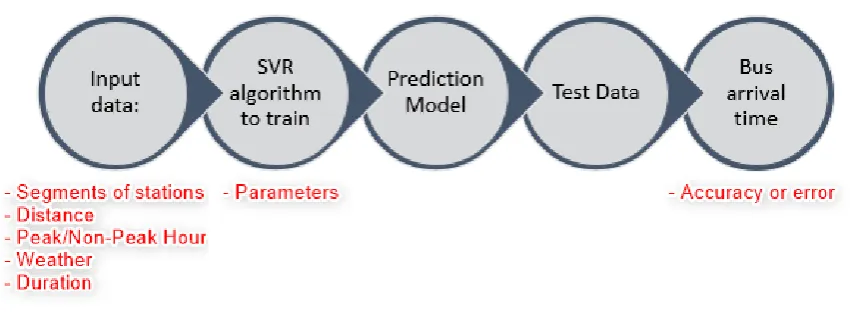
There are 5 input features that consist of segments of bus stations, duration of the journey from a station to the next station, the distance, time segment of whether the bus operates during peak hour or non-peak hour, and lastly the weather data. All the input features are used in the training of the model. Generally, a part of the input dataset is used as a train set and trained by using the SVR algorithm to get the bus arrival time prediction model, while the other part of the dataset is used as a test set to check on the accuracy or error of the prediction.
Figure 3. The overview of the methodology used in this paper. Data is processed in the Python programming environment.
the objective of this paper. For instance, the Pandas library is used to perform data cleansing on the Comma-Separated Values (CSV) file, and the Scikit-Learn library includes different algorithms for machine learning purposes, such as classification, regression and clustering.
Generally, the Radial Basis Function (RBF) kernel has been recommended and used by researchers for bus arrival time prediction [26]. Hence, the RBF kernel is used in this work and the full equation of SVR is as follows:
𝑦 = ∑𝑚𝑖=1(𝛼𝑖− 𝛼𝑖∗)𝑒𝑥𝑝(−𝛾||𝑥 − 𝑥𝑖||^2 ) + 𝑏 (15)
There are 3 parameters that need to be specified, namely C, ε, and γ. The experiment is run multiple times to determine the optimum parameters. By using the same parameters, training data with weather data can be compared against the training data without the weather data to understand whether the weather data is useful in predicting bus arrival time.
The dataset used in this work includes the inspection data of PJ City Bus route PJ03, which is operated by MBPJ. Approximately 350 bus trips between 02 June 2019 and 08 June 2019 were inspected to collect the data. Trip inspection data includes a sequence of bus stations, bus station names, the coordinate of the bus stations, timestamps and the distance covered from the previous station to the next station. The data is used by MBPJ to perform an inspection of the quality of operation of the urban City Bus. The data was recorded by using a mobile logging application on a mobile device specifically designed and developed for the bus driver. As soon as the bus driver signed in the mobile application by using the designated ID, the application identifies the bus driver and the bus plate number as well as the GPS location. When the bus arrives at a station, the bus driver presses a button on the application to log location and check the time, while the application calculates the distance covered from the previous check time. All the information is sent to and stored in the server. Due to the fact that logging needs to be performed manually, human error and machine error are unavoidable. Some trips are not completely logged or logged at the wrong location or time by the bus driver, and it is possible that the application error has caused certain trips that did not get logged at all.
Route PJ03 is located in Petaling Jaya and it covers a total length of 9.4KM via 23 bus stations, the operation starts from 6 AM to 12 AM midnight. Approximate time to travel from the first station to the last station is within 29 to 35 minutes under the most ideal situation where traffic is smooth.
Figure 10. The route of PJ03 on Google Maps. The blue flags are the bus stations.
3. Results
3.1Data preprocessing
In order to get the input features needed for model training, the data was preprocessed. First, the dataset was cleaned up in Python, whereby all non-ASCII text and all rows that contain missing data were removed. Then PJ03 was segmented into 22 segments, in which segment 1 covered the first station – LRT Taman Bahagia station to the second station of the route – Rumah No. 57 station, while segment 2 covered the second station to the third station – Petronas (OPP) stations. The same rule applies to the rest of the segments and stations. Figure 11 shows segments of the route and the corresponding stations.
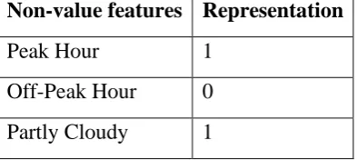
Time is divided into 2 categories, namely peak and non-peak hours. Peak hour spans from morning 8 AM to 11 AM and 5 PM to 8 PM, while the rest is considered as off-peak hours. The duration in seconds for each of the segments of each trip has been calculated by minus off the check time of the previous station from the check time of the current station. For instance, check the time of station 1 is 1:00 p.m., while check time for station 2 is 1:01 p.m., so the duration would be 60 seconds. There are 3 types of weather – partly cloudy, thunder and rain. The weather data has been added into the input dataset according to the period that corresponds to the weather dataset accordingly. Due to the machine error or the human (bus driver) error, the distance of the same segment can be found differently for each trip. It’s unlikely but still possible to have a slight variation in the distance recorded through action such as cut queue during bad traffic conditions. Nevertheless, all the input features needed to train the models, which are segments, distance, peak or non-peak hour, weather and duration are fully prepared by this step. Table 1 below summarizes the value representing non-value features in the dataset:
Table 1. Table showing value representing the non-value features in the dataset.
Non-value features Representation
Peak Hour 1
Off-Peak Hour 0
Thunder 2
Rain 3
Figure 11. Route PJ03 consists of 23 bus stations showing each of the segments covered in this paper.
Figure 12 shows the average duration a bus takes to move from one station to the next during off-peak and peak hours. The figure shows a general trend whereby a longer time is taken during peak hours compared to that during the off-peak hours. For example, a bus on average takes 102.39 seconds to move from station 2 to station 3 (segment 2) during off-peak hours, but it takes 119.21 seconds during peak hours. That means, due to the peak hours, it takes 16.82 seconds more. The highest difference shows in segment number 10. The reason behind that this segment may face the most traffic congestion or maybe the highest number of passengers take the ride from this station (number 9) in peak hours.
0 20 40 60 80 100 120 140
1 2 3 4 5 6 7 8 9 10 11 12 13 14 15 16 17 18 19 20 21 22
Du
ra
tio
n
(s
econ
d
s)
Segment number
Off Peak hour
Figure 12. Average duration a bus takes from one station to the next in peak and off-peak hours.
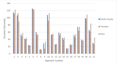
Figure 13 shows the average duration a bus takes to move from one station to the next with the variations of weather (as the importance has been given to the weather conditions, the peak hours or the off-peak hours issues are not considered here). The figure shows the effects of the weather on the bus traveling duration. From the figure, it is shown that the rain slows down the overall speed of the bus. In other words, the bus takes a longer duration to reach from one station to another due to rain. For example, in segment 20 (from station 20 to 21), when the weather is partly cloudy it takes on average 98.62 seconds, for the thunder, it is 97.24 seconds and 109.22 seconds while it is rain. In summary, it can be said that weather condition has the effect (though it is not significant) on the bus traveling duration, especially rain increases the arrival time of the bus.
Figure 13. Effect of the weather in duration a bus takes from one station to the next
3.2 Feature Scaling
Before feeding the data into the model, it needs to be scaled as the range of every input feature can be very different. For example, a duration range can be tens to thousands of seconds while peak hour and non-peak hours are represented by 1 and 0, respectively. Huge discrepancies between the input features can cause a fitting issue as a feature with a huge number may get different weights than a feature with a small number. Min-max scaling is used to scale the value of the data used in this paper between 0 and 1 as a means to improves the prediction model. The min-max scaling equation can be written as following [27]:
𝑥𝑖𝑛 = 𝑥𝑖−𝑚𝑖𝑛(𝑥𝑖)
𝑚𝑎𝑥(𝑥𝑖)−min(𝑥𝑖) (16)
where 𝑥𝑖𝑛 is the scaled value. This can be done by calling the built-in function of the Scikit-learn preprocessing library: skScikit-learn. preprocessing.MinMaxScaler.
3.3 Training of model
Prior to the training of the model, the dataset has been split into a train set and test set by using the built-in function of the Scikit-learn library: sklearn.model_selection.train_test_split.
0 20 40 60 80 100 120 140
1 2 3 4 5 6 7 8 9 10 11 12 13 14 15 16 17 18 19 20 21 22
Du
ra
tio
n
(Se
co
n
d
s)
Segment number
Partly Cloudy
Thunder
75% of the dataset has been categorized as a training dataset for the training of model while 25% of the dataset has been categorized as a test dataset for testing of the model.
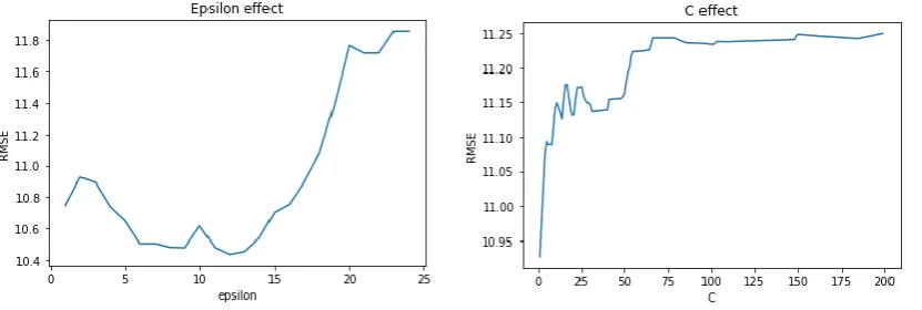
To train the model, the training dataset is fed into the SVR algorithm from the Scikit-learn library. There are a few parameters that need to be specified: C, Epsilon and Gamma value during the training of the model. They are set to default value during the first training, where C = 1, Epsilon = 0.1 and Gamma = ‘Auto’. Gamma value is kept as ‘Auto’ for the rest of the project as ‘Auto’ indicates (1/number of features). The best values for C and Epsilon of each segment are obtained through the reliable grid-search method [26]. After the first model is trained by using the default parameters, the model is tested by using the test dataset. The accuracy of the model is evaluated via the root mean squared error (RMSE) where it shows the difference of the predicted duration and the actual duration in the test set. The equation of RMSE can be represented as:
𝑅𝑀𝑆𝐸 (𝑆𝑒𝑐) = √∑ (𝑇𝐴,𝑖− 𝑇𝑃,𝑖)
2 𝑛
𝑖
𝑛 (17)
Where 𝑇𝐴,𝑖 is the actual duration, 𝑇𝑃,𝑖 is the predicted duration and n is the number of samples. The RMSE shows the difference in predicted duration and actual duration in seconds. A graph is plotted by having a range of different Epsilon value, to determine the lowest RMSE. Next, the Epsilon value that produced the lowest RMSE is passed into the next graph where a range of C values are plotted against RMSE to determine the lowest RMSE. The value of C and Epsilon that produced the lowest RMSE are fed into the SVR algorithm again to train the model. The model is evaluated again and the process of determining the value of C and Epsilon is repeated until the RMSE doesn’t get lower with other values. The whole model training process is repeated with training data without the weather data but with the same SVR parameters.
Figure 14. The graph showing the lowest RMSE of certain Epsilon and C value.
3.4 Performance of the model
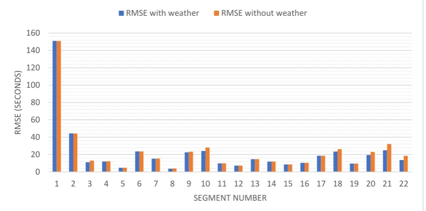
Figure 15. Performance of the model evaluated by using the test dataset. Lower RMSE means better performance(accuracy).
4. Discussion of the Model Performance
Generally, the SVR prediction model is showing good identification ability as 21 out of 22 road segments are having RMSE of lower than 45 seconds except for segment 1. That indicates the predicted duration for a bus to travel from one station to the next station is having lower than 45 seconds of error. This performance of the model in this work is better than Yang’s finding [28] where the average RMSE of all segments of road was around 40 seconds compared to the average RMSE of the prediction model of this work which is around 22 seconds (Figure 15 shows the comparison).
Figure 15. Comparison of average RMSE of this work with Yang’s work
In real life situation, the ETA of the bus to the next station can be computed as the check time at the previous station plus the predicted duration:
ETA (Station 2) = Check time (Station 1) + Predicted duration
However, the large RMSE of model prediction for segment 1 in comparison to the rest of the segments leaves a lot to be desired in performance-wise. This may be caused by a large range of duration from segment 1 in the training dataset, hence affecting the model prediction ability. One possibility that may attribute to the big duration range is the passenger flow. Passenger flow will affect the dwell time at the station since it’s located in the Light Rail Transit (LRT) station where there might be many passengers getting onto the bus, depending on the time of arrival of the LRT train intersect with the arrival of the bus. Human error or machine error
0 20 40 60 80 100 120 140 160
1 2 3 4 5 6 7 8 9 10 11 12 13 14 15 16 17 18 19 20 21 22
R MS E ( SE CO N DS ) SEGMENT NUMBER
RMSE with weather RMSE without weather
0 10 20 30 40 50
This work Yang's work [28]
mentioned previously could cause flawed data collection as well which could negatively impact the training of the prediction model. It was found that the weather data didn’t affect the performance as much as expected, as the largest difference of the model performance is only up to 5 seconds. This may be due to the limited data samples. Data samples that show changes in the weather are insufficient in this work and therefore the weather data has limited influence on the prediction model. From date 02-06-2019 to 08-06-2019, more than 75% of the time is partly cloudy, and the rest of the time is rain and thunder. There shall be a longer period of data that shows more rain and thunder weather for the weather to become an input feature with more weight.
Overall, the SVR prediction model for this paper performed relatively well with its low average RMSE but it’s not without its limitations, and its limitation will be discussed in the next section. The dataset used in this work can be found in [29].
Training of the model is always better with cleaner and well-structured data. The current model is trained by using only a week's worth of data samples as the authority does not provide more data due to their privacy and security issues. There’s the opportunity of increasing the performance of the model if more data samples are available.
5. Conclusions
One of the main issues nowadays for bus operators is that the ETA is not accurate and it deviates from actual ETA by too much, and this discourages riders and so ridership is affected in the long run, hence the purpose of this paper is to develop a machine learning model that may provide more accurate ETA. SVR, which is based on the SVM classifier model, is chosen for this paper. The SVR model developed in this paper has displayed good prediction ability. One of the characteristics of SVR is that only a small amount of dataset is needed to train the model with the considerable performance and generalization capability. Input features for the training of the model include segments, distance, weather, peak or non-peak hour are used to predict the travel duration for the segments. The data has been categorized into peak and non-peak hours based on the time the record is logged. Different types of hourly weather data have been assigned to each of the samples as well based on the log time. RBF kernel is chosen for this paper. By using the test dataset, the model is able to achieve 22 seconds of RMSE which is better than the result obtained in previous studies. Overall, SVR may be a feasible model for ETA prediction but it needs to be trained and tested vigorously with more data and features.
6. Acknowledgments
This work is supported by the Partnership Grant RK004-2017 & CR-UM-SST-DCIS-2018-01 between University of Malaya and Sunway University; and the Pioneer Scientist Incentive Fund (PSIF), UCSI University, through Research Grant no: Proj-2019-In-FOBIS-023.
7. Author Contributions
Conceptualization, Ng Seong Yik; Data curation, Wahidah Md Shah; Investigation, Kok-Lim Alvin Yau; Methodology, Ismail Ahmedy; Project administration, Tarak Nandy; Validation, Ismail Ahmedy and Mohammad Asif Hossain; Visualization, Kok-Lim Alvin Yau; Writing – original draft, Rafidah Md Noor; Writing – review & editing, Raenu Kolandaisamy.
Conflicts of Interest
The authors declare that there are no conflicts of interest regarding the publication of this paper.
[1] Urban Gateway, “Effect of Urbanisation,” 2019. [Online]. Available: https://www.urbangateway.org/document/effects-urbanisation. [Accessed: 05-Oct-2019].
[2] M. N. Borhan et al., “Predicting the use of public transportation: a case study from Putrajaya, Malaysia,” Sci. World J., vol. 9, 2014.
[3] N. . Aris, “Number of Malaysians using vehicles to increase 1.4 times by 2030,” FMT News, 2018. [Online]. Available: https://www.freemalaysiatoday.com/category/nation/2018/11/22/number-of-malaysians-using-vehicles-to-increase-1-4-times-by-2030/. [Accessed: 05-Oct-2019].
[4] Ministry of Transport Malaysia, “Transport Statistics Malaysia 2017,” 2017. [Online]. Available: http://www.mot.gov.my/en/Statistik Tahunan Pengangkutan/Transport Statistics Malaysia 2017.pdf. [Accessed: 05-Oct-2019].
[5] Invest KL Malaysia, “Kuala Lumpur’s Public Transport System All Set to Evolve to the Next Level.,” 2016. [Online]. Available: http://www.investkl.gov.my/Relevant_News-@Kuala_Lumpur_Public_Transport_System_All_Set_to_Evolve_to_the_Next_Level.aspx. [Accessed: 05-Oct-2019].
[6] The World Bank, "The High Toll of Traffic Injuries: Unacceptable and Preventable", World Bank Group
Open Knowledge Repository, 2017. Retrieved from
https://openknowledge.worldbank.org/bitstream/handle/10986/29129/HighTollofTrafficInjuries.pdf?se quence=5&isAllowed=y
[7] The Star, "Loke: Use public transport to reduce subsidy", 2019, Retrieved from https://www.thestar.com.my/news/nation/2019/06/14/loke-use-public-transport-to-reduce-subsidy, [8] Borhan, M.N., Ibrahim, A.N.H., Syamsunur, D., and Rahmat, R.A.,"Why Public Bus is a Less Attractive
Mode of Transport: A Case Study of Putrajaya, Malaysia". Periodica Polytechnica Transportation Engineering, 47(1), 82-90, 2019. https://doi.org/10.3311/PPtr.9228
[9] Department of Statistics Malaysia, "Press Release: State Socioeconomic Report 2018", Department of
Statistics Malaysia, 2019. Retrieved from
https://www.dosm.gov.my/v1/index.php?r=column/pdfPrev&id=a0c3UGM3MzRHK1N1WGU5T3pQ NTB3Zz09
[10] Official Portal of Selangor State Government,"Perkhidmatan Bas Selangor Percuma", 2019. Retrieved from https://www.selangor.gov.my/index.php/pages/view/1181
[11] Bernama, "38.6 million users have benefited from Smart Selangor Bus Service". Malaysiakini, 2019. Retrieved from https://www.malaysiakini.com/news/491432
[12] MBPJ, “PJ Transportation”, 2016. Retrieved from https://www.pjtransport.my
[13] Menon, P., and Selva, M.N.T., “New app for Smart Selangor bus and routes”. The Star Online, 2017. Retrieved from https://www.thestar.com.my/metro/metro-news/2017/11/08/new-app-for-smart-selangor-bus-and-routes#E6sLhavEBeL3iICb.99
[14] Jade, C.., “New routes and app for PJ City Bus service”. The Star Online. 2017. Retrieved from https://www.thestar.com.my/metro/metro-news/2017/10/26/new-routes-and-app-for-pj-city-bus-service-users-can-also-track-bus-location-and-estimated-arrival-t#pDP18H3jereyEKBR.99
[15] Department of Statistics Malaysia, “Compendium of Environment Statistic 2018”. Department of
Statistics Malaysia, 2018. Retrieved from
https://dosm.gov.my/v1/index.php?r=column/cthemeByCat&cat=162&bul_id=U3p3RVY0aGtGS08yT DY2cEpraDFlUT09&menu_id=NWVEZGhEVlNMeitaMHNzK2htRU05dz09
[16] Altinkaya, M., and Zontul, M., “Urban Bus Arrival Time Prediction: A Review of Computational Models”. International Journal of Recent Technology and Engineering (IJRTE), Volume 2, Issue 4, 2013. [17] Fan, W., and Gurmu, Z., “Dynamic Travel Time Prediction Models for Buses Using Only GPS Data”.
International Journal of Transportation Science and Technology, vol 4-2015. 353 – 366, 2015.
[18 ] Pan, J., Dai, X., Xu, X., Li, Y., “A Self-Learning Algorithm For Predicting Bus Arrival Time Based on Historical Data Model”, College of Computer Science and Technology, Zhejiang University of Technology, proceedings of IEEE CCIS2012, 1112-1116, 2012.
[19] Gurmu, Z.K., Nall & Perkins Inc, Fan, W.D., “Artificial Neural Network Travel Time Prediction Model for Buses Using Only GPS Data”, Journal of Public Transportation, Vol. 17, No. 2, 2014.
[21] Mayo, H., Punchihewa, H., Emile. J., and Morrison, J., “History of Machine Learning”, Imperial College London, 2018. Retrieved from https://www.doc.ic.ac.uk/~jce317/history-machine-learning.html [22] Amita, J., Singh, J.S., and Kumar, G.P., “Prediction of Bus Travel Time Using Artificial Neural
Network”. International Journal for Traffic and Transport Engineering, 2015, 5(4), 410 – 424, 2015. http://dx.doi.org/10.7708/ijtte.2015.5(4).06
[23] Smola, A.J., and Scholkopf, B.., “A tutorial on support vector regression”, Statistics and Computing 14,
199-222, 2004.
[24] Berwick, Robert, “An Idiot’s guide to Support Vector Machines (SVMs)”. Massachvsetts Institvte of Technology, Department of Electrical Engineering and Computer Science, 2010.
http://web.mit.edu/6.034/wwwbob/svm.pdf
[25] Reddy, K.K., Kumar, B.A., and Vanajakshi, L., “Bus travel time prediction under high variability conditions”, Current Science, Vol. 111(4), 2016.
[26] Bin, Y., Zhong-zhen, Y., Kang, C. and Bo, Y., “Hybrid Model for Prediction of Bus Arrival Times at Next Station”, Journal of Advanced Transportation, 44, 193-204, 2010. https://doi.org/10.1002/atr.136 [27] Scikit-learn, “Scikit-learn: Machine Learning in Python”, 2019. Retrieved 5th October from
https://scikit-learn.org/stable/index.html
[28] Yang, M., Chen, C., Wang, L., Yan, X. and Zhou, L., “Bus Arrival Time Prediction Using Support Vector Machine with Genetic Algorithm”, Neural Network World 3/2016, 205-217, 2016. https://doi.org/10.14311/NNW.2016.26.011
[29] NG Seong Yik, “Research-Project Dataset”, Retrieved from https://github.com/nsyik/Research-Project [Accessed: 05-Oct-2019].
[30] Rashid, Z., Mon, C. S., & Kolandaisamy, R. (2019, February). Proposing a Development of Geolocation
Mobile Application for Airport Pickup of International Students PickUp. In Proceedings of the 2019 8th