R E S E A R C H
Open Access
Joint source and relay design for MIMO
multi-relay systems using projected gradient
approach
Apriana Toding
1, Muhammad RA Khandaker
2and Yue Rong
3*Abstract
In this paper, we develop the optimal source precoding matrix and relay amplifying matrices for non-regenerative multiple-input multiple-output (MIMO) relay communication systems with parallel relay nodes using the projected gradient (PG) approach. We show that the optimal relay amplifying matrices have a beamforming structure. Exploiting the structure of relay matrices, an iterative joint source and relay matrices optimization algorithm is developed to minimize the mean-squared error (MSE) of the signal waveform estimation at the destination using the PG approach. The performance of the proposed algorithm is demonstrated through numerical simulations.
Keywords: MIMO relay; Parallel relay network; Beamforming; Non-regenerative relay; Projected gradient
1 Introduction
Recently, multiple-input multiple-output (MIMO) relay communication systems have attracted much research interest and provided significant improvement in terms of both spectral efficiency and link reliability [1-17]. Many works have studied the optimal relay amplifying matrix for the source-relay-destination channel. In [2,3], the optimal relay amplifying matrix maximizing the mutual informa-tion (MI) between the source and destinainforma-tion nodes was derived, assuming that the source covariance matrix is an identity matrix. In [4-6], the optimal relay amplify-ing matrix was designed to minimize the mean-squared error (MSE) of the signal waveform estimation at the destination.
A few research has studied the joint optimization of the source precoding matrix and the relay amplifying matrix for the source-relay-destination channel. In [7], both the source and relay matrices were jointly designed to maxi-mize the source-destination MI. In [8,9], source and relay matrices were developed to jointly optimize a broad class of objective functions. The author of [10] investigated the
*Correspondence: [email protected]
3Department of Electrical and Computer Engineering, Curtin University of Technology, Bentley, WA 6102, Australia
Full list of author information is available at the end of the article
joint source and relay optimization for two-way MIMO relay systems using the projected gradient (PG) approach. The source and relay optimization for multi-user MIMO relay systems with single relay node has been investigated in [11-14].
All the works in [1-14] considered a single relay node at each hop. In general, joint source and relay precoding matrices design for MIMO relay systems with multiple relay nodes is more challenging than that for single-relay systems. The authors of [15] developed the optimal relay amplifying matrices with multiple relay nodes. A matrix-form conjugate gradient algorithm has been proposed in [16] to optimize the source and relay matrices. In [17], the authors proposed a suboptimal source and relay matrices design for parallel MIMO relay systems by first relaxing the power constraint at each relay node to the sum relay power constraints at the output of the second-hop channel and then scaling the relay matrices to satisfy the individual relay power constraints.
In this paper, we propose a jointly optimal source pre-coding matrix and relay amplifying matrices design for a two-hop non-regenerative MIMO relay network with multiple relay nodes using the PG approach. We show that the optimal relay amplifying matrices have a beamform-ing structure. This new result is not available in [16]. It generalizes the optimal source and relay matrices design
from a single relay node case [8] to multiple parallel relay nodes scenarios. Exploiting the structure of relay matrices, an iterative joint source and relay matrices optimization algorithm is developed to minimize the MSE of the signal waveform estimation. Different to [17], in this paper, we develop the optimal source and relay matrices by directly considering the transmission power constraint at each relay node. Simulation results demonstrate the effective-ness of the proposed iterative joint source and relay matri-ces design algorithm with multiple parallel relay nodes using the PG approach.
The rest of this paper is organized as follows. In Section 2, we introduce the model of a non-regenerative MIMO relay communication system with parallel relay nodes. The joint source and relay matrices design algo-rithm is developed in Section 3. In Section 4, we show some numerical simulations. Conclusions are drawn in Section 5.
2 System model
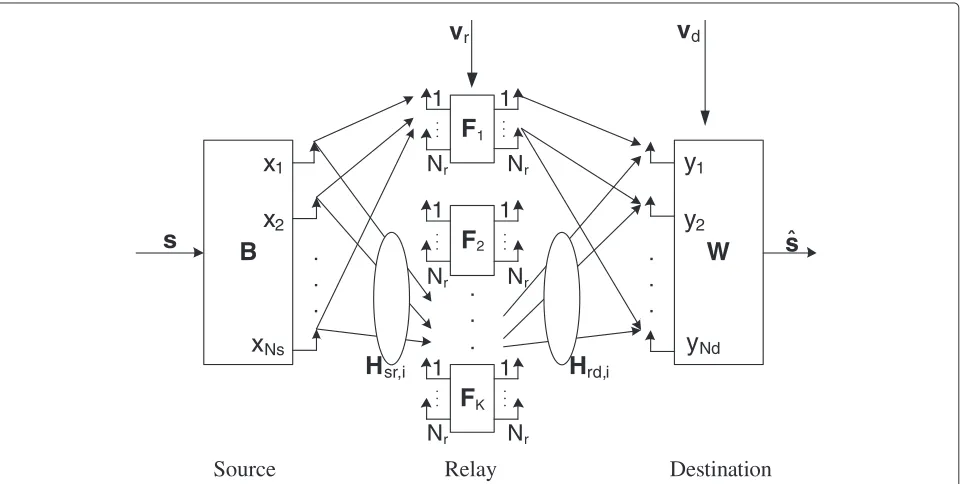
In this section, we introduce the model of a two-hop MIMO relay communication system consisting of one source node,K parallel relay nodes, and one destination node as shown in Figure 1. We assume that the source and destination nodes haveNsandNdantennas, respectively,
and each relay node hasNrantennas. The generalization
to systems with different number of antennas at each relay node is straightforward. Due to its merit of simplicity, a linear non-regenerative strategy is applied at each relay node. The communication process between the source and destination nodes is completed in two time slots. In
the first time slot, theNb×1(Nb≤Ns)modulated source symbol vectorsis linearly precoded as
x=B s, (1)
where B is an Ns × Nb source precoding matrix. We
assume that the source signal vector satisfies EssH = INb, whereIn stands for ann×nidentity matrix,(·)
H is the matrix (vector) Hermitian transpose, and E[·] denotes statistical expectation. The precoded vectorxis transmit-ted toK parallel relay nodes. TheNr×1 received signal
vector at theith relay node can be written as
yr,i=Hsr,ix+vr,i, i=1,· · ·,K, (2) whereHsr,iis theNr×NsMIMO channel matrix between
the source and theith relay nodes andvr,i is the additive Gaussian noise vector at theith relay node.
In the second time slot, the source node is silent, while each relay node transmits the linearly amplified signal vector to the destination node as
xr,i=Fiyr,i, i=1,· · ·,K, (3) whereFiis theNr×Nramplifying matrix at theith relay
node. The received signal vector at the destination node can be written as
yd= K
i=1
Hrd,ixr,i+vd, (4)
whereHrd,iis theNd×NrMIMO channel matrix between
the ith relay and the destination nodes, and vd is the
additive Gaussian noise vector at the destination node.
Source
Relay
Destination
s
F
1F
2F
KW
B
.
.
.
.
.
.
.
.
.
y
1x
1x
2x
Nsy
2y
NdH
sr,i1
H
rd,i1
1
1
1
1
N
rN
rN
rN
rN
rN
rv
rv
dˆ
s
•• • • • •
• • • • • •
• • • • • •
Substituting (1) to (3) into (4), we have
nel matrix between the source node and all relay nodes, Hrd
Hrd,1,Hrd,2,· · ·,Hrd,K
is anNd×KNr channel
matrix between all relay nodes and the destination node, F bd[F1,F2,· · ·,FK] is the KNr × KNr block diago-nal equivalent relay matrix,vr
vTr,1,vTr,2,· · ·,vTr,KT is obtained by stacking the noise vectors at all the relays,
˜
H HrdFHsrBis the effective MIMO channel matrix
of the source-relay-destination link, andv˜ HrdFvr +
vd is the equivalent noise vector. Here, (·)T denotes
the matrix (vector) transpose, bd[·] constructs a block-diagonal matrix. We assume that all noises are indepen-dent and iindepen-dentically distributed (i.i.d.) Gaussian noise with zero mean and unit variance. The transmission power consumed by each relay node (3) can be expressed as
Etrxr,ixHr,i
where tr(·)stands for the matrix trace.
Using a linear receiver, the estimated signal waveform vector at the destination node is given by ˆs = WHyd,
whereWis anNd×Nbweight matrix. The MSE of the
signal waveform estimation is given by
MSE=tr Eˆs−s sˆ−sH whereC˜ is the equivalent noise covariance matrix given byC˜ = Ev˜v˜H = HrdFFHHHrd+INd. The weight matrix W which minimizes (7) is the Wiener filter and can be written as
W=(H˜H˜H+ ˜C)−1H,˜ (8) where(·)−1denotes the matrix inversion. Substituting (8)
back into (7), it can be seen that the MSE is a function of FandBand can be written as
3 Joint source and relay matrix optimization In this section, we address the joint source and relay matrix optimization problem for MIMO multi-relay sys-tems with a linear minimum mean-squared error (MMSE) receiver at the destination node. In particular, we show that optimal relay matrices have a general beamforming
structure. Based on (6) and (9), the joint source and relay matrices optimization problem can be formulated as
min power constraint at the source node, while (12) is the power constraint at each relay node. Here,Ps > 0 and
Pr,i > 0,i =1,· · ·,K, are the corresponding power bud-get. Obviously, to avoid any loss of transmission power in the relay system when a linear receiver is used, there should beNb ≤ min(KNr,Nd). The problem (10)-(12) is
non-convex, and a globally optimal solution ofBand{Fi} is difficult to obtain with a reasonable computational com-plexity. In this paper, we develop an iterative algorithm to optimizeBand{Fi}. First, we show the optimal structure of{Fi}.
3.1 Optimal structure of relay amplifying matrices For given source matrixBsatisfying (11), the relay matri-ces{Fi}are optimized by solving the following problem:
min
Let us introduce the following singular value decompo-sitions (SVDs): rank of a matrix. Based on the definition of matrix rank,
Rs,i≤min(Nr,Nb)andRr,i ≤min(Nr,Nd). The following
theorem states the structure of the optimal{Fi}.
Theorem 1.Using the SVDs of (15), the optimal struc-ture ofFias the solution to the problem (13)-(14) is given by
Fi=Vr,iAiUs,Hi, i=1,· · ·,K, (16)
whereAiis an Rr,i×Rs,imatrix, i=1,· · ·,K .
The remaining task is to find the optimal Ai, i = 1,· · ·,K. From (31) and (32) in Appendix 1, we can equiv-alently rewrite the optimization problem (13)-(14) as
min
Both the problem (13)-(14) and the problem (17)-(18) have matrix optimization variables. However, in the for-mer problem, the optimization variableFi is anNr ×Nr
matrix, while the dimension ofAiisRr,i×Rs,i, which may be smaller than that ofFi. Thus, solving the problem (17)-(18) has a smaller computational complexity than solving the problem (13)-(14). In general, the problem (17)-(18) is non-convex, and a globally optimal solution is difficult to obtain with a reasonable computational complexity. For-tunately, we can resort to numerical methods, such as the projected gradient algorithm [18] to find (at least) a locally optimal solution of (17)-(18).
Theorem 2.Let us define the objective function in (17) as f(Ai). Its gradient∇f(Ai)with respect toAican be cal-culated by using results on derivatives of matrices in [19] as
Proof. See Appendix 2.
In each iteration of the PG algorithm, we first obtain ˜
Ai = Ai−sn∇f(Ai)by movingAi one step towards the negative gradient direction off(Ai), wheresn > 0 is the step size. SinceA˜imight not satisfy the constraint (18), we need to project it onto the set given by (18). The projected matrixA¯iis obtained by minimizing the Frobenius norm ofA¯i− ˜Ai(according to [18]) subjecting to (18), which can be formulated as the following optimization problem:
min
Ai. Otherwise, the solution to the problem (20)-(21) can be obtained by using the Lagrange multiplier method, and the solution is given by
¯
whereλ >0 is the solution to the non-linear equation of
tr A˜i
Equation (22) can be efficiently solved by the bisection method [18].
The procedure of the PG algorithm is listed in Algorithm 1, where (·)(n) denotes the variable at the nth iteration,δ
n andsn are the step size parameters at thenth iteration, · denotes the maximum among the absolute value of all elements in the matrix, and ε is a positive constant close to 0. The step size parametersδnandsn are deter-mined by the Armijo rule [18], i.e.,sn = sis a constant through all iterations, while at thenth iteration,δnis set to beγmn. Here,m
nis the minimal non-negative integer that satisfies the following inequalityf A(in+1)
constants. According to [18], usuallyαis chosen close to 0, for example,α∈[ 10−5, 10−1], while a proper choice of
γ is normally from 0.1 to 0.5.
3.2 Optimal source precoding matrix
With fixed {Fi}, the source precoding matrix B is opti-mized by solving the following problem:
Algorithm 1 Procedure of applying the projected gradient algorithm to solve the problem (17)-(18)
1. Initialize the algorithm at a feasibleA(i0)for
whereHHsrFHHHrdHrdFFHHHrd+INd
−1
HrdFHsr, and ˘
Pr,i Pr,i − tr
FiFHi
, i = 1,· · ·,K. Let us introduce BBH, and a positive semi-definite (PSD) matrix X withX INs +
1 2 12
−1
, whereA Bmeans that A−Bis a PSD matrix. By using the Schur complement [20], the problem (23)-(25) can be equivalently converted to the following problem:
min
X, tr(X)−Ns+Nb (26)
s.t.
X INs INs INs +
1 2 12
0, (27)
tr( )≤Ps, 0, (28)
trFiHsr,i HHsr,iFHi
≤ ˘Pr,i, i=1,· · ·,K. (29)
The problem (26)-(29) is a convex semi-definite pro-gramming (SDP) problem which can be efficiently solved by the interior point method [20]. Let us introduce the eigenvalue decomposition (EVD) of = U UH, where is a R × R eigenvalue matrix with R =
rank( ). If R = Nb, then from = BBH, we have
B = U 1
2. IfR > N
b, the randomization technique
[21] can be applied to obtain a possibly suboptimal solu-tion of B with rank Nb. If R < Nb, it indicates that the system (channel) cannot supportNbindependent data streams, and thus, in this case, a smaller Nb should be
chosen in the system design.
Now, the original joint source and relay optimization problem (10)-(12) can be solved by an iterative algorithm as shown in Algorithm 2, where(·)(m) denotes the vari-able at themth iteration. This algorithm is first initialized at a random feasible B satisfying (11). At each itera-tion, we first update {Fi} with fixed Band then update B with fixed{Fi}. Note that the conditional updates of each matrix may either decrease or maintain but cannot increase the objective function (10). Monotonic conver-gence of{Fi} and Btowards (at least) a locally optimal solution follows directly from this observation. Note that in each iteration of this algorithm, we need to update the relay amplifying matrices according to the proce-dure listed in Algorithm 1 at a complexity order of OKNd3+N3
r +Nb3
and update the source precoding matrix through solving the SDP problem (26)-(29) at a complexity cost that is at mostO Ns2+K+13.5using interior point methods [22]. Therefore, the per-iteration computational complexity order of the proposed algo-rithm isO KNd3+Nr3+Nb3+Ns2+K+13.5. The overall complexity of this algorithm depends on the num-ber of iterations until convergence, which will be studied in the next section.
Algorithm 2 Procedure of solving the problem (10)-(12)
1. Initialize the algorithm at a feasibleB(0)satisfying constraint (11); setm=0.
2. For fixedB(m), obtain{Fi}(m)by solving the problem
(17)-(18) using the PG algorithm.
3. UpdateB(m+1)by solving the problem (26)-(29) with known{Fi}(m).
4. IfB(m+1)−B(m) ≤ε, then end. Otherwise, let
m:=m+1and go to step 2.
4 Simulations
In this section, we study the performance of the pro-posed jointly optimal source and relay matrix design for MIMO multi-relay systems with linear MMSE receiver. All simulations are conducted in a flat Rayleigh fading environment where the channel matrices have zero-mean entries with variancesσs2/Ns andσr2/(KNr) forHsr and
Hrd, respectively. For the sake of simplicity, we assume Pr,i =Pr,i=1,· · ·,K. The BPSK constellations are used to modulate the source symbols, and all noises are i.i.d. Gaussian with zero mean and unit variance. We define SNRs = σs2PsKNr/Ns and SNRr = σr2PrNd/(KNr) as
the signal-to-noise ratio (SNR) for the source-relay link and the relay-destination link, respectively. We transmit 1000Ns randomly generated bits in each channel
real-ization, and all simulation results are averaged over 200 channel realizations. In all simulations, we setNb=Ns= Nr = Nd = 3, and the MMSE linear receiver in (8) is
employed at the destination for symbol detection. In the first example, a MIMO relay system withK =
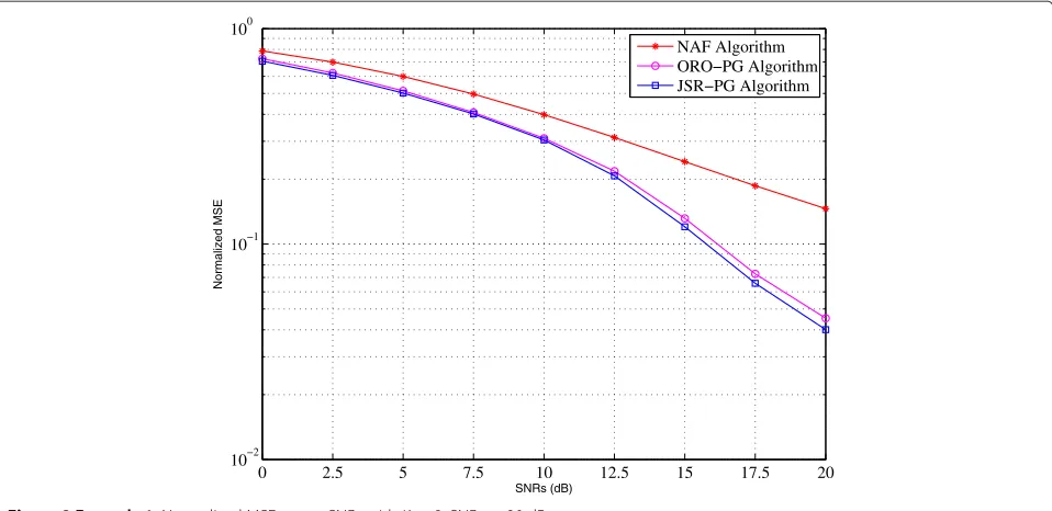
3 relay nodes is simulated. We compare the normalized MSE performance of the proposed joint source and relay optimization algorithm using the projected gradient (JSR-PG) algorithm in Algorithm 2, the optimal relay-only algorithm using the projected gradient (ORO-PG) algo-rithm in Algoalgo-rithm 1 withB=√Ps/NsINs, and the naive amplify-and-forward (NAF) algorithm. Figure 2 shows the normalized MSE of all algorithms versus SNRs for
SNRr =20 dB. While Figure 3 demonstrates the
normal-ized MSE of all algorithms versus SNRrfor SNRsfixed at
20 dB. It can be seen from Figures 2 and 3 that the JSR-PG and ORO-JSR-PG algorithms have a better performance than the NAF algorithm over the whole SNRsand SNRr
range. Moreover, the proposed JSR-PG algorithm yields the lowest MSE among all three algorithms.
The number of iterations required for the JSR-PG algo-rithm to converge to ε = 10−3 in a typical channel realization are listed in Table 1, where we set K = 3 and SNRr = 20 dB. It can be seen that the JSR-PG
0 2.5 5 7.5 10 12.5 15 17.5 20
10−2
10−1
100
SNRs (dB)
Normalized MSE
NAF Algorithm ORO−PG Algorithm JSR−PG Algorithm
Figure 2Example 1.Normalized MSE versus SNRswithK=3, SNRr=20 dB.
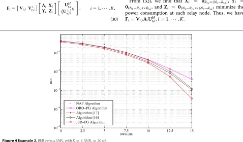
In the second example, we compare the bit error rate (BER) performance of the proposed JSR-PG algorithm in Algorithm 2, the ORO-PG algorithm in Algorithm 1, the suboptimal source and relay matrix design in [17], the one-way relay version of the conjugate gradient-based source and relay algorithm in [16], and the NAF algorithm. Figure 4 displays the system BER versus SNRsfor a MIMO
relay system withK =3 relay nodes and fixed SNRrat 20
dB. It can be seen from Figure 4 that the proposed JSR-PG algorithm has a better BER performance than the existing algorithms over the whole SNRsrange.
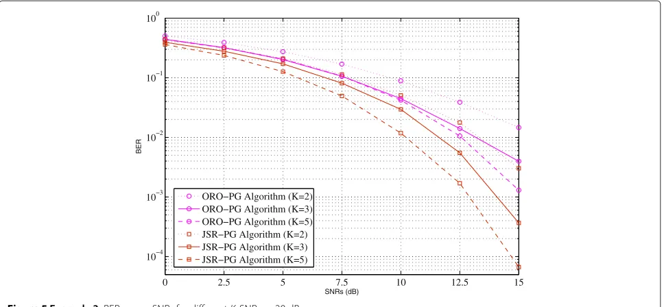
In the third example, we study the effect of the num-ber of relay nodes to the system BER performance using the JSR-PG and ORO-PG algorithms. Figure 5 displays the system BER versus SNRs withK = 2, 3, and 5 for fixed
SNRr at 20 dB. It can be seen that at BER = 10−2, for
both the ORO-PG algorithm and JSR-PG algorithm, we can achieve approximately 3-dB gain by increasing from
K = 2 toK = 5. It can also be seen that the perfor-mance gain of the JSR-PG algorithm over the ORO-PG algorithm increases with the increasing number of relay nodes.
0 2.5 5 7.5 10 12.5 15 17.5 20 10−2
10−1 100
SNRr (dB)
Normalized MSE
NAF Algorithm ORO−PG Algorithm JSR−PG Algorithm
Table 1 Iterations required until convergence in the JSR-PG algorithm
SNRs(dB) Iterations
0 3
2.5 3
5 3
7.5 4
10 4
12.5 5
15 5
17.5 5
20 6
5 Conclusions
In this paper, we have derived the general structure of the optimal relay amplifying matrices for linear non-regenerative MIMO relay communication systems with multiple relay nodes using the projected gradient approach. The proposed source and relay matrices mini-mize the MSE of the signal waveform estimation. The sim-ulation results demonstrate that the proposed algorithm has improved the MSE and BER performance compared with existing techniques.
Appendices
Appendix 1
Proof of Theorem 1
Without loss of generality,Fican be written as
Fi=Vr,i V⊥r,i
Ai Xi
Yi Zi
UHs,i
U⊥s,iH
, i=1,· · ·,K,
(30)
where V⊥r,i(V⊥r,i)H = INr −Vr,iVHr,i, U⊥s,i
U⊥s,iH = INr − Us,iUHs,i, such thatV¯r,i
Vr,i,V⊥r,i
andU¯s,i
Us,i,U⊥s,i
areNr ×Nr unitary matrices. Matrices Ai,Xi,Yi,Zi are arbitrary matrices with dimensions ofRr,i×Rs,i,Rr,i×(Nr− Rs,i),(Nr−Rr,i)×Rs,i,(Nr−Rr,i)×(Nr−Rs,i), respectively. Substituting (15) and (30) back into (13), we obtain that Hrd,iFiHsr,iB = Ur,ir,iAis,iVHs,i andHrd,iFiFiHHHrd,i = Ur,ir,i
AiAHi +XiXHi
r,iUHr,i. Thus, we can rewrite (13) as
MSE tr
⎛ ⎝
INb+
K
i=1
Vs,is,iAHi r,iUHr,i
×
K
i=1
Ur,ir,i
AiAHi +XiXHi
r,iUHr,i+INd
−1
× K
i=1
Ur,ir,iAis,iVHs,i −1⎞
⎠. (31)
It can be seen that (31) is minimized by Xi = 0Rr,i×(Nr−Rs,i),i=1,· · ·,K.
Substituting (15) and (30) back into the left-hand side of the transmission power constraint (14), we have
trFi
Hsr,iBBHHHsr,i+INr
FHi =trAi
2
s,i+IRs,i
AHi +Yi
2
s,i+IRs,i
YHi +XiXHi +ZiZHi
, i=1,· · ·,K.
(32)
From (32), we find that Xi = 0Rr,i×(Nr−Rs,i), Yi =
0(Nr−Rr,i)×Rs,i, andZi = 0(Nr−Rr,i)×(Nr−Rs,i) minimize the
power consumption at each relay node. Thus, we have Fi=Vr,iAiUs,Hi,i=1,· · ·,K.
0 2.5 5 7.5 10 12.5 15 10−5
10−4 10−3 10−2 10−1
SNRs (dB)
BER
NAF Algorithm ORO−PG Algorithm Algorithm [17] Algorithm [16] JSR−PG Algorithm
0 2.5 5 7.5 10 12.5 15
Proof of Theorem 2
Let us define Zi Kj=1,j =iUr,jr,jAjs,jVHs,j andYi (33) can be written as
f(Ai)=tr
Competing interests
The authors declare that they have no competing interests.
Acknowledgements
The work of Yue Rong was supported in part by the Australian Research Council’s Discovery Projects funding scheme (project number DP140102131). The first author (Apriana Toding) would like to thank the Higher Education Ministry of Indonesia (DIKTI) and the Paulus Christian University of Indonesia (UKI-Paulus) of Makassar, Indonesia, for providing her with a PhD scholarship at Curtin University, Perth, Australia.
Author details
1Department of Electrical Engineering, Universitas Kristen Indonesia Paulus, Jln.
Perintis Kemerdekaan No 28 Daya, Makassar 90243, Indonesia.2Department of
Electronic and Electrical Engineering, University College London, Gower Street, London WC1E 7JE, UK.3Department of Electrical and Computer Engineering,
Curtin University of Technology, Bentley, WA 6102, Australia.
Received: 5 May 2014 Accepted: 1 September 2014 Published: 15 September 2014
References
1. B Wang, J Zhang, A Høst-Madsen, On the capacity of MIMO relay channels. IEEE Trans. Inf. Theory.51, 29–43 (2005)
2. X Tang, Y Hua, Optimal design of non-regenerative MIMO wireless relays. IEEE Trans. Wireless Commun.6, 1398–1407 (2007)
3. O Muñoz-Medina, J Vidal, A Agustín, Linear transceiver design in nonregenerative relays with channel state information. IEEE Trans. Signal Process.55, 2593–2604 (2007)
4. W Guan, H Luo, Joint MMSE transceiver design in non-regenerative MIMO relay systems. IEEE Commun. Lett.12, 517–519 (2008)
5. G Li, Y Wang, T Wu, J Huang, Joint linear filter design in multi-user cooperative non-regenerative MIMO relay systems. EURASIP J. Wireless Commun. Netw.2009, 670265 (2009)
6. Y Rong, Linear non-regenerative multicarrier MIMO relay communications based on MMSE criterion. IEEE Trans. Commun.58, 1918–1923 (2010) 7. Z Fang, Y Hua, JC Koshy, Joint source and relay optimization for a
non-regenerative MIMO relay, inProc. IEEE Workshop Sensor Array Multi-Channel Signal Process(Waltham, WA, USA, 12–14 July 2006, pp. 239–243 8. Y Rong, X Tang, Y Hua, A unified framework for optimizing linear
non-regenerative multicarrier MIMO relay communication systems. IEEE Trans. Signal Process.57, 4837–4851 (2009)
9. Y Rong, Y Hua, Optimality of diagonalization of multi-hop MIMO relays. IEEE Trans. Wireless Commun.8, 6068–6077 (2009)
10. Y Rong, Joint source and relay optimization for two-way linear
non-regenerative MIMO relay communications. IEEE Trans. Signal Process. 60, 6533–6546 (2012)
11. MRA Khandaker, Y Rong, Joint transceiver optimization for multiuser MIMO relay communication systems. IEEE Trans. Signal Process.60, 5997–5986 (2012)
12. MRA Khandaker, Y Rong, Joint source and relay optimization for multiuser MIMO relay communication systems, inProceedings of the 4th
International Conference on Signal Processing and Communication Systems
Gold Coast, Australia, 13–15 Dec 2010
13. H Wan, W Chen, Joint source and relay design for multiuser MIMO nonregenerative relay networks with direct links. IEEE Trans. Veh. Technol. 61, 2871–2876 (2012)
14. J Zeng, Z Chen, L Li, Iterative joint source and relay optimization for multiuser MIMO relay systems, inProceedings of the IEEE Vehicular Technology ConferenceQuebec City, QC, Canada, 3–6 Sept 2012 15. AS Behbahani, R Merched, AM Eltawil, Optimizations of a MIMO relay
network. IEEE Trans. Signal Process.56, 5062–5073 (2008)
16. C-C Hu, Y-F Chou, Precoding design of MIMO AF two-way multiple-relay systems. IEEE Signal Process. Lett.20, 623–626 (2013)
17. A Toding, MRA Khandaker, Y Rong, Joint source and relay optimization for parallel MIMO relay networks. EURASIP J. Adv. Signal Process.2012, 174 (2012)
18. DP Bertsekas,Nonlinear Programming, 2nd edn, Athena Scientific, Belmont,1999)
19. KB Petersen, MS Petersen, The Matrix Cookbook. http://www2.imm.dtu. dk/pubdb/p.php?3274. Accessed 9 Sept 2014
20. S Boyd, L Vandenberghe,Convex Optimization. (Cambridge University Press, Cambridge, 2004)
21. P Tseng, Further results on approximating nonconvex quadratic optimization by semidefinite programming relaxation. SIAM J. Optim. 14(1), 268–283 (2003)
22. Y Nesterov, A Nemirovski,Interior Point Polynomial Algorithms in Convex Programming, (SIAM, Philadelphia, 1994)
doi:10.1186/1687-1499-2014-151
Cite this article as:Todinget al.:Joint source and relay design for MIMO
multi-relay systems using projected gradient approach.EURASIP Journal on
Wireless Communications and Networking20142014:151.
Submit your manuscript to a
journal and benefi t from:
7Convenient online submission
7Rigorous peer review
7Immediate publication on acceptance
7Open access: articles freely available online
7High visibility within the fi eld
7Retaining the copyright to your article