R E S E A R C H
Open Access
Blind source separation with optimal
transport non-negative matrix factorization
Antoine Rolet
1*, Vivien Seguy
1, Mathieu Blondel
2and Hiroshi Sawada
2Abstract
Optimal transport as a loss for machine learning optimization problems has recently gained a lot of attention. Building upon recent advances in computational optimal transport, we develop an optimal transport non-negative matrix factorization (NMF) algorithm for supervised speech blind source separation (BSS). Optimal transport allows us to design and leverage a cost between short-time Fourier transform (STFT) spectrogram frequencies, which takes into account how humans perceive sound. We give empirical evidence that using our proposed optimal transport, NMF leads to perceptually better results than NMF with other losses, for both isolated voice reconstruction and speech denoising using BSS. Finally, we demonstrate how to use optimal transport for cross-domain sound processing tasks, where frequencies represented in the input spectrograms may be different from one spectrogram to another.
Keywords: NMF, Speech, BSS, Optimal transport
1 Introduction
Source separation is the task of separating a mixed signal into different components, usually referred to as sources. In the context of sound processing, it can be used to separate speakers whose voices have been recorded simul-taneously. Blind source separation (BSS) aims at doing so with only sound data, that is without information such as the time when each source is active or the location of the sources with respect to the recording devices. A common way to address this task is to decompose the signal spectrogram by non-negative matrix factorization ([15], NMF), as proposed for example by [25] as well as [29]. Denotingx˜j,i, the (complex) short-time Fourier
trans-form (STFT) coefficient of the input signal at frequency binjand time framei, andXits magnitude spectrogram defined asxj,i = |˜xj,i|, the BSS problem can be tackled by
solving the NMF problem
min
D(1)...D(N),W(1)...W(N) t
i=1
xi, N
k=1
D(k)w(k)i
*Correspondence:[email protected]
Work performed during an internship at NTT Communication Science Laboratories
1Graduate School of Informatics, Kyoto University, Yoshida Honmachi, Kyoto,
Japan
Full list of author information is available at the end of the article
where N is the number of sources, t is the number of time windows,xi is the ith column ofX, andis a loss
function. Each dictionary matrixD(k)and weight matrix W(k) are related to a single source. In a supervised set-ting, each source has training data and all the D(k)s are learned in advance during a training phase. At test time, given a new signal, separated spectrograms are recov-ered from theD(k)s andW(k)s and corresponding signals can be reconstructed with suitable post-processing. Sev-eral loss functionshave been considered in the litera-ture, such as the squared Euclidean distance [15,25], the Kullback-Leibler divergence [15,28], or the Itakura-Saito divergence [9,24].
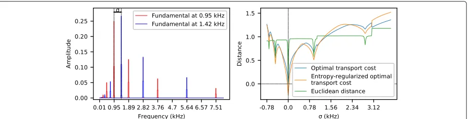
In the present article, we propose to useoptimal trans-port as a loss between spectrograms to perform super-vised speech BSS with NMF. Optimal transport is defined as the minimum cost of moving the mass from one his-togram to another. By taking into account a transportation cost between frequencies, this provides a powerful metric to compare STFT spectrograms. One of the main advan-tages of using optimal transport as a loss is that it can quantify the amplitude of a frequency shift noise, com-ing for example from quantization or the tuncom-ing of a musical instrument. Other metrics such as the Euclidean distance or Kullback-Leibler divergence, which compare spectrogram element-wise, are almost blind to this type of noise (see Fig.1). Another advantage over element-wise
Fig. 1Comparison of Euclidean distance and (regularized) optimal transport losses. Synthetic musical notes are generated by putting weight on a fundamental, and exponentially decreasing weights on its harmonics and sub-harmonics, and finally convoluting with a Gaussian. Left: examples of the spectrograms of two such notes. Right: (regularized) optimal transport loss and Euclidean distance from the note of fundamental 0.95 kHz (red line on the left plot) to the note of fundamental 0.95 kHz+ σ, as functions ofσ. The Euclidean distance varies sharply whereas the optimal transport loss captures more smoothly the change in the fundamental. The variations of the optimal transport loss and its regularized version are similar, although the regularized one can become negative
metrics is that optimal transport enables the use of differ-ent quantizations, i.e., frequency supports, at training and test times. Indeed, the frequencies represented on a spec-trogram depend on the sampling rate of the signal and the time windows used for its computation, both of which can change between training and test times. With optimal transport, we do not need to re-quantize the training and testing data so as they share the same frequency support: optimal transport is well defined between spectrograms with distinct supports as long as we can define a trans-portation cost between frequencies. Finally, the optimal transport framework enables us to generalize the Wiener filter, a common post-processing for source separation, by using optimal transport plans, so that it can be applied to data quantized on different frequencies.
NMF with an optimal transport loss was first proposed by [23]. They solved this problem by using a bi-convex for-mulation and relied on an approximation of optimal trans-port based on wavelets [27]. Recently, [22] proposed fast algorithms to compute NMF with an entropy-regularized optimal transport loss, which are more flexible in the sense that they do not require any assumption on the fre-quency quantization or on the cost function used. How-ever, their approach requires all columnsxi of the input
matrix to be normalized so that they sum to 1. Normal-izing all time frames is not desirable in sound processing tasks because time frames with low energy usually corre-spond to noise, and it would amplify their contribution to the objective.
Similarly, optimal transport was proposed as a loss for performing principal component analysis (PCA) [3, 5], a task which is closely related to dictionary learning and NMF. However, rather than learning a dictionary on data histograms directly, they proposed to learn a dictio-nary on optimal mappings between a reference histogram and these histograms. Their approach was motivated by
the Riemannian geometry of the space of histograms equipped with the optimal transport distance w.r.t., the square Euclidean cost. Since their framework is limited to the square Euclidean cost, their approach is unsuitable for spectrogram data where a specifically designed cost should be considered as we advocate in this article.
Using optimal transport as a loss between spectrograms was also proposed by [10] under the name “optimal spec-tral transportation.” They developed a novel method for unsupervised music transcription which achieves state-of-the-art performance. Their method relies on a cost matrix designed specifically for musical instruments, allowing them to use Diracs as dictionary columns. That is, theyfixeach dictionary column to a vector with a single non-zero entry and learn only the corresponding coeffi-cients. This trivial structure of the dictionary results in efficient coefficient computation. However, this approach cannot be applied as is to speech separation since it relies on the assumption that a musical note can be represented as its fundamental. It also requires designing the cost of moving the fundamental to its harmonics and neighbor-ing frequencies. Because human voices are intrinsically more complex, it is therefore necessary to learn both the dictionary and the coefficients, i.e., solve full NMF problems.
1.1 Our contributions
losses. We show that optimal transport yields compara-ble results to other losses for BSS, where the sources to separate are voices. Moreover, we show that optimal transport achieves better results than other losses for learning a “universal” voice model, i.e., a model that can be applied to any voice, regardless of the speaker. We use this universal voice model to perform speech denois-ing, which is BSS where one of the source is a voice and the other is noise. Finally, we show how to use our framework for cross-domain BSS, where frequencies rep-resented in the test spectrograms may be different from the ones in the dictionary. This may happen for exam-ple when train and test data are recorded with different equipment, or when the STFT is computed with different parameters.
1.2 Notations
We denote matrices in uppercase, vectors in bold lower-case, and scalars in lowercase. IfMis a matrix,Mis its transpose,mi is itsith column,mj itsjth row and ImM
its image. 1n denotes the all-ones vector inRn; when the
dimension can be deduced from context, we simply write 1. For two matrices Aand B of the same size, we denote their inner productA,B:=tr(AB). We denotenthe
We start by introducing optimal transport, its entropy reg-ularization, which we will use as the loss, and previous works on optimal transport NMF. For a more comprehen-sive overview of optimal transport from a computational perspective, see [20].
2.1 Optimal transport
Exact optimal transport. Let a ∈ m,b ∈ n. The
polytope of transportation matrices betweena andb is defined as portation cost betweenaandbis defined as
OT(a,b)= min yi as features andaandbas the quantization weights of
the data onto these features. In sound processing appli-cations, the vectorsyi are real numbers corresponding to
the frequencies of the spectrogram andaandbare their
corresponding magnitude. By computing the minimal transportation cost between frequencies of two spectro-grams, optimal transport exhibits variations in accordance with the frequency noise involved in the signal genera-tive process, which results for instance from the tuning of musical instruments or the subject’s condition in speech processing.
Unnormalized optimal transport. In this work, we wish to define optimal transport whenaandbare non-negative but not necessarily normalized. Note that the transporta-tion polytope is not empty as long asaandbsum to the same value:U(a,b)= ∅iif a1= b1. Hence, we define optimal transport between possibly unnormalized vectors aandbas,
Computing the optimal transport cost (1) amounts to solve a linear program (LP) which can be done with spe-cialized versions of the simplex algorithm with worst-case complexity inOn3lognwhenn = m[19]. When con-sidering OT as a loss between histograms supported on more than a few hundred bins, such computation becomes quickly intractable. Moreover, using OT as a loss involves differentiating OT, which is not differentiable everywhere. Hence, one would have to resort to subgradient meth-ods. This would be prohibitively slow since each iteration would require to obtain a subgradient at the current iter-ate, which requires to solve the LP (1).
Entropy-regularized optimal transport. To remedy these limitations, [7] proposed to add an entropy regu-larization term to the optimal transport objective, thus making the OT loss differentiable everywhere and strictly convex. This entropy-regularized optimal transport has since been used in numerous works as a loss for diverse tasks ([11,12,22], see for example).
Let γ > 0, we define the (unnormalized) entropy-regularized OT betweena∈Rm+,b∈Rn+as
OTγ(x,y)= max
z≥0 z1=x1
y,z −OTγ(x,z).
Cuturi and Peyré [8] showed that its value and gradient can be computed in closed form:
OTγ(x,y)=γE(x)+ x, logKα,
NMF can be cast as an optimization problem of the form
min
where both D and W are optimized at train time, and D is fixed at test time. When is OT, problem (2) is convex inW andDseparately, but not jointly. It can be solved by alternating full optimization with respect toW andD. Each resulting sub-problem is a very high dimen-sional linear program with many constraints [23], which is intractable with standard LP solvers even for short sound signals. In addition, convergence proofs of suchalternate minimizationmethods for NMF typically assume strictly convex sub-problems (see e.g., [2,30] Prop. 2.7.1), which is not the case when using non-regularized OT as a loss.
To address this issue, [22] proposed to use OTγ instead and showed how to solve each sub-problem in the dual using fast gradient computations. Formally, they tackle problems of the form:
whereR1andR2are convex regularizers that enforce non-negativity constraints, andnis the(n−1)-dimensional
simplex.
It was shown that each sub-problem of (3) with either D or W fixed has a smooth Fenchel-Rockafellar dual, which can be solved efficiently, leading to a fast overall algorithm. However, their definition of optimal trans-port requires inputs and reconstructions to have a - 1 norm equal to 1. This is achieved by normalizing the input beforehand, restricting the columns ofDandW to the simplex, and using as regularizers negative entropies defined on the simplex:
They showed that the coefficients and dictionary can be updated according to the following duality results.
Coefficient update. For D fixed, the optimizer of min
We can solve problem (5) with accelerated gradient descent [18] and recover the optimal weight matrix with the primal-dual relationship (4). The value and gradient of the convex conjugate of Rwith respect to its second variable are:
R(ρ,x)=ρlogex/ρ,1
∇xR(ρ,x)=
ex/ρ ex/ρ,1.
Dictionary update. For W fixed, the optimizer of
min
Likewise, we can solve problem (7) with accelerated gra-dient descent and recover the optimal dictionary matrix with the primal-dual relationship (6).
These duality results allow us to go from a constrained primal problem for which each evaluation of the objec-tive and its gradient requires solving an optimal transport problem, to a non-constrained dual problem whose objec-tive and gradient can be evaluated in closed form. The primal constraintsxi1 = DWi1andDWi ≥ 0∀iare
enforced by the primal-dual relationship. Moreover, the use of an entropy regularization, withγ >0, makes OTγ
smooth with respect to its second variable.
3 Method
3.1 Signal separation with NMF
We use a supervised BSS setting similar to the one described in [25]. For each source k, we have access to training data X(k), on which we learn a dictionary D(k) with NMF
Then, given the STFT spectrum of a mixture of sourcesX, we reconstruct separated spectrogramsX(k)= D(k)W(k)fork=1,. . .NwhereW(k)s are the solutions of
The separated spectrogramsXˆ(k)are then reconstructed from eachX(k)with the process described in Section3.4.
In practice at test time, the dictionaries are concate-nated in a single matrix D = D(k)Nk=1, and a single matrix of coefficientsWis learned, which we decompose asW = W(k)Nk=1. This allows us to focus on problems
Voice-voice separation. We use the method described to separate the voices of two speakers on the same sound-track. In this case, we have access to training data on each speaker.
Denoising with universal models. We can also use BSS to denoise speech data. In this case, we do not have access to training data for speakers in the test set. We only have access to data of other speakers, which we use to learn a “universal” voice model, as in [29]. We also have two sources, the first one being a speaker and the second one a noise source. Here, we are only interested in the reconstruction of the voice, that isXˆ(1).
3.2 Non-normalized optimal transport NMF
Normalizing the columns of the input X, as in [22], is not a good option in the context of signal processing since frames with low amplitudes are typically noise and it would amplify them. Although this is not a problem for learning the coefficient matrixW, which is a column-independant process, it would increase the contribution of noise when learning the dictionary matrixD.
With our definition of optimal transport however, inputs are not required to be in the simplex, but only to have the same- 1 norm. With this definition, the con-vex conjugate OT of OT and its gradient still have the same value as in [8], and we can simply relax the con-straint on W to beW ≥ 0 in problem (3). We keep a
simplex constraint on the columns of the dictionaryDso that each update is guaranteed to stay in a compact set. We useR1 = −ρ1E, a negative entropy defined on the non-negative orthant as the coefficient matrix regularizer, and forR2, we keep the non-negative entropy defined on the simplex. The problem then becomes
min
This change of constraints yields the same dictionary update as in Section2.2, Eq.6. However, the coefficient updates need to be modified as follows.
Theorem 1(coefficient update) For D fixed, the opti-mizer of
ProofThe terms in the sum are independent on the columns of XandW. Let us thus solve it separately for each column. Let 0≤i≤t, the problem is
These conditions are sufficient for strong duality to hold, with the primal-dual relation w∗ ∈ ∇R1−Dg ([21], Example 11.41) .
The concave conjugate of R1 and its gradient can be evaluated with:
3.3 Cost matrix design
In order to compute optimal transport on spectrogams and perform NMF, we need a cost matrixC, which rep-resents the cost of moving weight from frequencies in the original spectrogram to frequencies in the reconstructed spectrogram. Schmidt and Olsson [25] use the mel scale to quantize spectrograms, relying on the fact that the per-ceptual difference between frequencies is smaller for the high frequency than for the low frequency domain. Fol-lowing the same intuition, we propose to map frequencies to a log-domain and apply a cost function in that domain. Letfjbe the frequency of thejth bin in an input data
spec-trogram, where 1≤ j≤m. Letfˆˆjbe the frequency of the ˆ
jth bin in a reconstruction spectrogram, where 1≤ ˆj≤n. We define the cost matrixC∈Rm×nas
cjˆj=logλ+fj
−log
λ+ ˆfˆjp
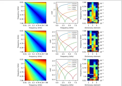
with parametersλ≥0 andp>0. Since the mel scale is a log scale, it is included in this definition for some param-eterλ. Some illustrations of our cost matrix for different values ofλare shown in Fig.2, withp=0.5. It shows that
with our definition, moving weights locally is less costly for high frequencies than low ones and that this effect can be tuned by selectingλ.
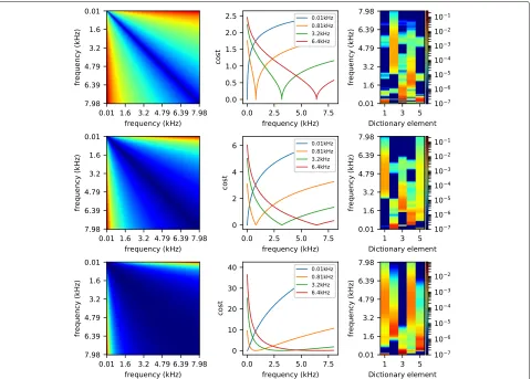
Figure3shows the effect ofpon the learned dictionar-ies. Usingp=0.5 yields a cost that is more spiked, leading to dictionary elements that can have several spikes in the same frequency bands, whereasp ≥ 1 tends to produce smoother dictionary elements.
Note that with this definition andp ≥ 1 ,C is a dis-tance matrix to the powerpwhen the source and target frequencies are the same. Ifp = 0.5,Cis the point-wise square-root of a distance matrix and as such is a distance matrix itself, OT(., .)1/p.
Parametersp = 0.5 andλ = 100 yielded better results for blind source separation on the validation set and were accordingly used in all our experiments.
3.4 Post-processing
Wiener filter. In the case where the reconstruction is in the same frequency domain as the original signal, the classical way to recover each voice in the time domain is to apply a Wiener filter. LetX be the original Fourier
Fig. 3Influence of the powerpof the cost matrix. Left, cost matrix; center, sample lines of the cost matrix; right, dictionary learned on the validation data. Top ,p=0.5; center,p=1; bottom,p=2
spectrum,X(1) andX(2) the separated spectra such that X ≈ X(1)+X(2). The Wiener filter builds Xˆ(1) = X
X(1)
X(1)+X(2) andXˆ(2) = X X (2)
X(1)+X(2), before applying the
original spectra’s phase and performing the inverse STFT.
Generalized filter. We propose to extend this filtering to the case whereX(1)andX(2)are not in the same domain as X. This may happen for example if the test data is recorded using a different sample frequency, or if the STFT is per-formed with a different time-window than the train data. In such a case, D(1) and D(2) are in the domain of the train data and are X(1) and X(2), butX is in a different domain, and its coefficients correspond to different sound frequencies. As such, we cannot use Wiener filtering.
Instead, we propose to use the optimal transportation matrices to produce separated signalsXˆ(1)andXˆ(2)in the same domain asX. LetT(i)∈ arg min
∈U
xi,x(i1)+x(i2)
C,. With
Wiener filtering, xi is decomposed into its components
generated by x(i1) and x(i2). We use the same idea and separate the transport matrixT(i)into:
T(i)(1)=T(i)diag
x(i1)
x(i1)+x(i2)
T(i)(2)=T(i)diag
x(i2)
x(i1)+x(i2)
T(i)(1)
resp.T(i)(1)
is a transport matrix between x
(1)
i
x(i1)+x(i2)
resp. x
(2)
i
x(i1)+x(i2)
andxˆi(1)
resp.xˆi(2)
, where
ˆ
xi(1)=T(i)
x(i1)
x(i1)+x(i2)
ˆ
xi(2)=T(i)
x(i2)
x(i1)+x(i2)
ˆ
Because of this property, the couple
ˆ xi(1),xˆi(2)
is a fix point of the Wiener Filter.
Separated signal reconstruction. Separated sounds are reconstructed by inverse STFT after applying either the Wiener filter or the generalized filter toX(1)andX(2).
4 Results
In this section, we present the main empirical findings of this paper. We start by describing the dataset that we used and the pre-processing we applied to it. We then show that the optimal transport loss allows us to have per-ceptually good reconstructions of single voices, even with few dictionary elements. We show that the optimal trans-port loss yields comparable results to other classical losses for voice-voice BSS with an NMF model. We also show that our generalized filter yields very similar results to the Wiener filter in the single-domain setting and can improve upon it in the cross-domain setting. Finally, we show that the optimal transport improves upon these other losses when using a universal voice model for voice denoising.
4.1 Dataset and pre-processing
Voice data. We evaluate our method on the English part of the Multi-Lingual Speech Database for Telephonome-try 1994 dataset1. The data consists of recordings of the voice of four males and four females pronouncing each 24 different English sentences. We split each person’s audio file time-wise into 25– 75% train-test data.
Noise data. For the speech denoising experiment, we consider 4 types of noises: cicadas, drums, subway, and sea. For each, we gathered one file for training and one file for testing from non-copyrighted sources on the internet2. We trimmed the training files so that they are approxi-mately 20 s long and made sure that test files were longer than the voice test sounds. Note that for each noise type, the training and testing files were gathered using the same keywords, but can still have quite a bit of variability.
Pre-processing. All sound files are re-sampled to 16 kHz and treated as mono signal. The signals are analyzed by STFT with a Hann window, and a window size of 1024, leading to 513 frequency bins ranging from 0–8 kHz. The constant coefficient is removed from the NMF analysis and added for reconstruction in post-processing.
Parameter selection. Hyper-parameters are selected on validation data consisting if the first male and female
voice, which are excluded from the evaluation set. We choose the parameters which yield the best SDR score in the voice-voice BSS experiment for these voices. We also use these voices as the training data for the universal voice model.
Initialization Initialization is performed by setting each value of the dictionary matrix as a random number picked uniformly in [ 0, 1]. It would be possible to set each dic-tionary column to the optimal transport barycenter (com-puted for example with [1]) of all the time frames of the training data, and adding Gaussian noise (separately for each column). However, we did not notice a significant improvement with this initialization, and we only report here the scores with completely random initialization so that the results are comparable to the other methods. When training a model for any loss, we perform the NMF four times and keep the model with minimum training loss to reduce the impact of random initialization.
4.2 NMF audio quality
We first show that using an optimal transport loss for NMF leads to better perceptual reconstruction of voice data. To that end, we evaluated the PEMO-Q score [13] of isolated test voices.
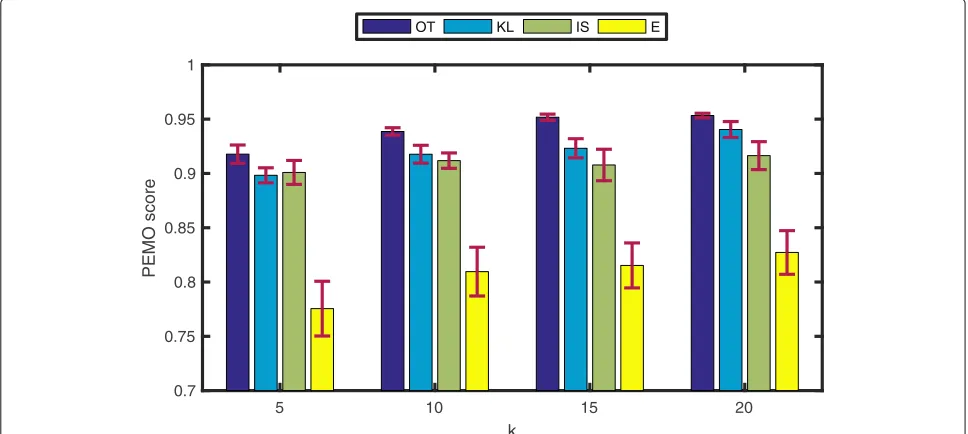
Personal voice model. Figure 4 shows the mean and standard deviation of the scores for k ∈ {5, 10, 15, 20} with optimal transport (OT), Kullback-Leibler (KL), Itakura-Saito (IS), or Euclidean (E) NMF. In this setting, the dictionaries are learned separately on the training data for each voice. These dictionaries are the same as in the following single-domain voice-voice separation exper-iment. The PEMO-Q score of optimal transport NMF is higher for any value ofk, although KL and IS results are still competitive. We found empirically that other scores such as SDR or SNR tend to be better for the Euclidean NMF, even though the reconstructed voices are clearly worse when listening to them (see Additional files 1 and 2). Optimal transport can reconstruct clear and intelligible voices with as few as five dictionary elements.
Fig. 4Perceptive quality score (personal voice model). Average and standard deviation of PEMO scores of reconstructed isolated voices, where the model is learned using separate training data for each voice with optimal transport (dark blue), Kullback-Leibler (light blue), Itakura-Saito (green), or Euclidean (yellow) NMF
two speakers become less important that the overall pat-terns of human voices. Indeed, the scores with optimal transport are very similar whether we use a universal or a personal voice model, whereas they drop significantly for the other losses when using a universal model.
4.3 Voice-voice blind source separation
We evaluate our blind source separation using the classical signal-to-distortion ratio (SDR) scores evaluated
on reconstructed audio files using the MatLab toolbox BSS eval v2.1 [32].
Single-domain blind source separation. We first use NMF to perform BSS in the case of mixtures of two voices, where we have training data for each voice. Here, the spectrograms of the training and test data represent the same frequencies: both the training and test data are pro-cessed in exactly the same way, so that at train and test
time(fi)i =
ˆ fi
i. We compare using the optimal
trans-port loss for NMF to the Kullback-Leibler divergence, the Itakura-Saito divergence, or the Euclidean distance. For baseline methods, we reconstruct the signal using a Wiener filter before applying inverse STFT. For optimal transport-based source separation, we evaluate separa-tion using either the Wiener filter or our generalized filter.
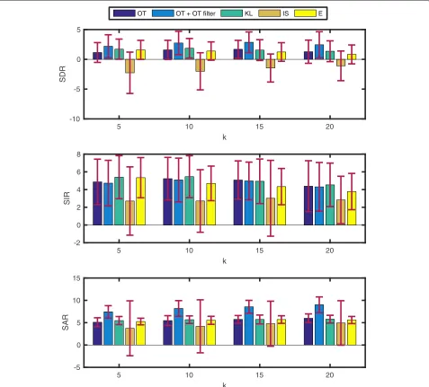
Figure 6 shows mean and standard deviation of the SDR, SIR, and SAR scores for each method. We can see that although KL NMF achieves a better SDR score, the variability is actually high and the results are comparable for all method.
Cross-domain blind source separation. In this experi-ment, we artificially generate spectrograms which repre-sent different frequencies for the training and test data by simply changing the STFT window size. For the training data, we use a window of size 512 and a window of size 800 for the test data.
Although (fi)i =
ˆ fi
i, we can still compute optimal
transport between the spectrograms, thanks to our cost matrix, and thus, we can use the trained dictionary as is to compute the weight matrix at test time.
In order to compute the weight matrix for the other losses however, we first need to re-quantize the dictionary matrix so that it represents the same frequencies as the
test data. We do it by assigning each frequency in the smaller spectrogram to its closest frequency in the larger one. This can be done with the simple linear operation
D←ADwith
ai,j= ⎧ ⎨ ⎩
1 ifj=min arg min
k |fi− ˆfk|
0 otherwise.
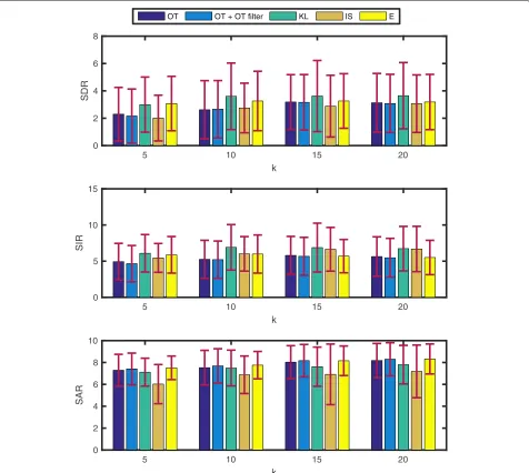
Figure 7 shows mean and standard deviation of the SDR, SIR, and SAR scores for each method. In the case of the optimal transport loss, we report both the result with the generalized filter, and the Wiener filter applied
toAX(k). We can see that the SDR scores have dropped a lot, except with the optimal transport loss combined to our generalized filter. We notice a similar effect on the signal-to-artifact ratio (SAR), meaning that the sep-aration process has created artifacts, which are actually very noticeable when listening to the reconstructed sound, except when using the generalized filter. This is probably due to the fact that the heuristic mapping process cancels a lot of frequencies which were in the test data.
4.4 Universal voice model for speech denoising
Setting We now use NMF to first learn a universal speech model and noise models and then apply these models for
Table 1Speech denoising SDR scores
OT OT + OT filter KL IS E
k k k k k
5 10 15 20 5 10 15 20 5 10 15 20 5 10 15 20 5 10 15 20
Cicada 7.7 8.8 8.9 8.4 7.3 8.0 8.6 8.1 7.7 7.9 7.9 7.9 7.7 7.9 7.6 7.7 7.9 8.0 7.9 7.5
±0.1 ±0.1 ±0.1 ±0.1 ±0.1 ±0.1 ±0.1 ±0.1 ±0.1 ±0.1 ±0.1 ±0.1 ±0.1 ±0.1 ±0.1 ±0.1 ±0.1 ±0.1 ±0.1 ±0.1
Drums 1.3 3.6 2.7 2.8 1.5 3.8 2.7 2.9 2.0 3.3 2.6 3.1 0.5 0.9 0.6 1.0 1.9 3.4 2.0 2.0
±0.6 ±0.7 ±0.7 ±0.5 ±0.5 ±0.6 ±0.7 ±0.6 ±0.3 ±0.7 ±0.4 ±0.4 ±0.2 ±0.1 ±0.1 ±0.0 ±0.6 ±0.5 ±0.4 ±0.3
Sea 0.0 1.5 3.3 1.8 0.0 1.8 3.3 1.9 1.6 3.4 4.6 4.3 1.6 3.0 3.7 3.5 3.5 4.1 4.4 3.8
±0.9 ±0.7 ±0.5 ±1.1 ±0.8 ±0.6 ±0.5 ±1.0 ±1.3 ±1.0 ±0.8 ±0.7 ±0.8 ±0.6 ±0.6 ±0.5 ±1.1 ±0.9 ±0.9 ±0.6
Subway 2.0 2.8 1.5 2.2 1.8 2.8 1.6 2.3 1.8 2.0 1.9 1.8 2.0 1.4 1.7 2.1 1.5 1.8 1.7 1.7
±1.1 ±0.9 ±0.9 ±1.2 ±1.0 ±1.0 ±0.9 ±1.2 ±1.3 ±1.6 ±0.9 ±0.9 ±0.6 ±0.3 ±0.3 ±0.4 ±1.9 ±1.2 ±1.0 ±0.9
The bold figure in each line indicates the best score for a specific noise
speech denoising. The universal speech model is learned on the concatenated training data of the first male and first female voices of our dataset. For each noise type, we learn a model with NMF on its training data. We then mix test voices with test noise with a pSNR of 0 and use our BSS approach to separate the voice. All the scores reported are evaluated on the voices only since reconstruction of the noise is not our goal here.
In this experiment, we kept the same parameters for the cost matrix of optimal transport as in the ones selected in the voice-voice BSS experiment. We report the scores for each dictionary sizekin{5, 10, 15, 20}.
Results Tables 1, 2 and3 show the SDR, SIR and SAR scores with their standard deviation for all methods and all noise types. We can see from Tables1and2that the opti-mal transport yields significantly better SDR and SIR than other methods for all noises except “sea.” This is consis-tent with our observation that the optimal transport loss allows to good reconstruction with a universal model.
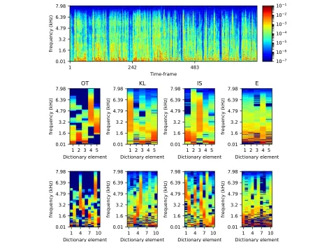
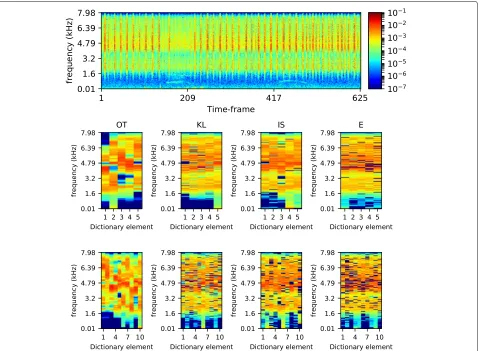
Dictionaries Figures 8 and 9 show the dictionaries learned for the universal voice model and the cicada noise, respectively, with all losses and a dictionary size of 5 and
10. The dictionaries learned with optimal transport tend to be smoother and maybe with less overlap between dictionary elements. They seem to have high activation on bands, rather than isolated frequencies, and each dictio-nary element has only a few bands with high activation. The IS loss seems to induce similar effect to a lesser extent, while the KL and even more so the Euclidean loss tend to be spiked, with a lot of spikes for a same dictionary element, and more redundancy between elements.
Running times. Our implementation of the method in Python with numpy on 3 CPU cores of 2.93 gHz takes about 3 min to fully learn a dictionary of 5 elements on the cicada training data, which is about 20 s long, leading to spectrograms inR512×724. Test times are around 2 min for sound files of around 50 s, which is not real time but close. We used rather tight convergence criteria in these experiments, and we believe that these times could be reduced by using better hardware (multi-core, GPUs) and looser convergence criteria. For comparison, computing times for the KL loss, with a similar alternate minimiza-tion scheme (with inner optimizaminimiza-tions performed with the multiplicative updates of [15]) and the same convergence
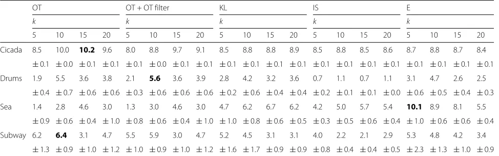
Table 2Speech denoising SIR scores
OT OT + OT filter KL IS E
k k k k k
5 10 15 20 5 10 15 20 5 10 15 20 5 10 15 20 5 10 15 20
Cicada 8.5 10.0 10.2 9.6 8.0 8.8 9.7 9.1 8.5 8.8 8.8 8.9 8.5 8.8 8.5 8.6 8.7 8.8 8.7 8.4
±0.1 ±0.0 ±0.1 ±0.1 ±0.1 ±0.0 ±0.1 ±0.1 ±0.1 ±0.1 ±0.1 ±0.1 ±0.1 ±0.1 ±0.1 ±0.1 ±0.1 ±0.1 ±0.1 ±0.1
Drums 1.9 5.5 3.6 3.8 2.1 5.6 3.6 3.9 2.8 4.2 3.2 3.6 0.7 1.1 0.7 1.1 3.1 4.7 2.6 2.5
±0.4 ±0.7 ±0.6 ±0.6 ±0.3 ±0.6 ±0.6 ±0.6 ±0.2 ±0.6 ±0.4 ±0.4 ±0.2 ±0.1 ±0.1 ±0.0 ±0.6 ±0.5 ±0.4 ±0.3
Sea 1.4 2.8 4.6 3.0 1.3 3.0 4.6 3.0 4.7 6.2 6.7 6.2 4.2 5.0 5.7 5.4 10.1 8.9 8.1 5.5
±0.9 ±0.6 ±0.4 ±1.0 ±0.8 ±0.6 ±0.4 ±1.0 ±1.0 ±0.8 ±0.6 ±0.5 ±0.3 ±0.5 ±0.6 ±0.4 ±1.0 ±0.6 ±0.6 ±0.4
Subway 6.2 6.4 3.1 4.7 5.5 5.9 3.0 4.7 5.2 4.5 3.1 3.1 4.0 2.2 2.1 2.9 5.3 4.8 4.2 3.4
±1.3 ±0.9 ±1.0 ±1.2 ±1.0 ±0.9 ±1.0 ±1.2 ±1.6 ±1.7 ±0.9 ±0.9 ±0.8 ±0.4 ±0.4 ±0.5 ±2.3 ±1.3 ±1.0 ±0.9
Table 3Speech denoising SAR scores
OT OT + OT filter KL IS E
k k k k k
5 10 15 20 5 10 15 20 5 10 15 20 5 10 15 20 5 10 15 20
Cicada 16.1 15.7 15.2 15.3 16.5 16.6 15.6 15.7 15.9 15.7 15.8 15.4 16.4 15.9 15.5 15.3 16.3 16.2 16.2 15.6
±0.3 ±0.3 ±0.2 ±0.2 ±0.3 ±0.4 ±0.2 ±0.2 ±0.3 ±0.3 ±0.3 ±0.2 ±0.4 ±0.3 ±0.3 ±0.2 ±0.4 ±0.3 ±0.3 ±0.3
Drums 12.5 9.0 11.6 11.1 12.9 9.5 11.8 11.4 11.7 12.1 13.4 14.0 17.9 17.4 20.7 19.9 9.9 10.5 12.7 13.7
±1.7 ±0.5 ±0.6 ±0.4 ±1.5 ±0.5 ±0.6 ±0.5 ±1.6 ±0.7 ±0.5 ±0.4 ±2.1 ±1.1 ±0.4 ±0.4 ±0.8 ±0.4 ±0.4 ±0.4
Sea 8.1 9.4 10.3 9.8 8.5 10.0 10.5 10.2 5.8 7.6 9.5 9.8 6.6 8.5 9.2 9.3 5.1 6.4 7.5 9.9
±1.8 ±0.9 ±0.7 ±1.0 ±1.8 ±0.9 ±0.7 ±1.0 ±1.4 ±1.3 ±1.2 ±1.0 ±1.5 ±0.9 ±0.7 ±1.1 ±1.4 ±1.1 ±1.1 ±1.1
Subway 5.0 6.3 8.6 7.1 5.4 6.8 8.8 7.3 5.9 7.1 10.0 9.5 7.8 11.6 13.6 11.9 5.0 6.3 6.8 8.3
±1.3 ±1.0 ±0.5 ±1.0 ±1.3 ±1.1 ±0.5 ±1.0 ±1.3 ±1.2 ±0.9 ±1.0 ±0.9 ±1.1 ±0.7 ±0.5 ±1.4 ±1.0 ±1.0 ±0.8
The bold figure in each line indicates the best score for a specific noise
criteria is about 50 s for training and about 20 s for testing.
5 Discussion
Regularization of the transport plan. In this work, we considered entropy-regularized optimal transport as
introduced by [7]. This allows us to get an easy-to-solve dual problem since its convex conjugate is smooth and can be computed in closed form. However, any convex reg-ularizer would yield the same duality results and could be considered as long as its conjugate is computable. For instance, the squared L2 norm regularization was
Fig. 9Noise dictionaries. Dictionaries learned for the cicada noise. Top row: spectrogram of the training data. Middle and bottom row: dictionaries learned with respectively 5 and 10 elements, with the optimal transport, Kullback-Leibler, Itakura-Saito, and Euclidean loss (from left to right)
considered in several recent works [4,26] and was shown to have desirable properties such as better numerical sta-bility or sparsity of the optimal transport plan. Moreover, similarly to entropic regularization, it was shown that the convex conjugate and its gradient can be computed in closed form [4].
Learning procedure. Following the work of [22], we solved the NMF problem with an alternating minimiza-tion approach, in which at each iteraminimiza-tion, a complete optimization is performed on either the dictionary or the coefficients. While this seems to work well in our exper-iments, it would be interesting to compare with smaller step approaches like in [15]. Unfortunately, such updates do not exist to our knowledge: gradient methods in the primal would be prohibitively slow since they involve solv-ingtlarge optimal transport problems at each iteration.
5.1 Future work
Sparsity Many works using NMF for sound processing add sparsity-inducing regularization to the NMF loss.
This is usually achieved with al1 regularization on the coefficient matrix W[16, 29]. We believe such sparsity would also benefit our approach, althoughl1 regulariza-tion cannot be applied directly. Indeed, we have con-straints of the form DWi1 = Xi1, and since all columns of D are in the simplex, this is equivalent to Wi1 = Xi1, so we already have a hard constraint on thel1 norm ofW. One solution to this problem is to use an “unbalanced” optimal transport loss [6,11], for which both input do not need to have the same total weight. Unbalanced versions of optimal transport as defined in [6] do not have an easy-to-compute convex conjugate to the best of our knowledge, but [12] casts unbalanced optimal transport into a regular optimal transport problem, and our approach should work with this loss.
each channel. A more interesting approach in our opinion would be to design a cost matrix which would encode the cost of moving power not only between frequencies but also between channels.
Optimal transport in other models. We believe optimal transport can improve upon other losses between spec-trograms in many sound processing tasks, as long as the loss is evaluated between spectrograms. For instance, one can use a speech-denoising auto-encoder as done by [14] and use the optimal transport loss with our proposed cost matrix on the reconstructed spectrograms. However, the simple linear model of NMF used in this paper allows us to have simple and easy-to-optimize duals. This is not the case with deep neural networks, and one would have to resort to more computationally involved primal gradient-based approaches as in [11] or [17].
6 Conclusion
We showed that using an optimal transport-based loss can improve performance of NMF-based models for voice reconstruction and separation tasks. We believe this is a first step towards using optimal transport as a loss for speech processing, possibly using more complicated models such as sparse NMF or deep neural networks. The versatility of optimal transport, which can compare spectrograms on different frequency domains, lets us use dictionaries on sounds that are not recorded or processed in the same way as the training set. This property could also be beneficial to learn common representations (e.g., dictionaries) for different datasets.
Endnotes
1http://www.ntt-at.com/product/speech2002/
2See availability of data section.
Additional files
Additional file 1:Reconstruction with optimal transport NMF. This WAV file contains the reconstructed test sentences of the male validation voice with optimal transport NMF and a dictionary of rank 5 (five columns), where the dictionary was learned on the training sentences of the same voice. (WAV 2831 kb)
Additional file 2:Reconstruction with Euclidean NMF. This WAV file contains the reconstructed test sentences of the male validation voice with Euclidean NMF and a dictionary of rank 5 (five columns), where the dictionary was learned on the training sentences of the same voice. (WAV 2831 kb)
Abbreviations
BSS: Blind source separation; E: Euclidean; IS: Itakura-Saito; KL: Kullback-Leibler; LP: Linear program; NMF: Non-negative matrix factorization; OT: Optimal transport; SAR: Signal-to-artifact ratio; SDR: Signal-to-distortion ratio; SIR: Signal-to-interference ratio; SNR: Signal-to-noise ratio; STFT: Short-time Fourier transform
Acknowledgements
The authors would like to thank Arnaud Dessein, who gave helpful insight on the cost matrix design.
Funding
The authors do not have any particular funding to declare.
Availability of data and materials
The voice dataset we used for our experiments is the English part of the Multi-Lingual Speech Database for Telephonometry 1994 dataset, distributed by NTT. Requests for the data are handled through the form athttp://www. ntt-at.com/product/speech2002/. The noise sound files we used were gathered onhttps://freesound.org/. We provide them in a zip archive in the following link: https://drive.google.com/file/d/1A9A3-Bfc6SvztZGA9wYcLJBCPzqWQUlx/view?usp=sharing.
Authors’ contributions
AR, VS, MB, and HS designed the research and wrote the paper. Experiments were performed by AR. All authors read and approved the final manuscript.
Competing interests
The authors declare that they have no competing interests.
Publisher’s Note
Springer Nature remains neutral with regard to jurisdictional claims in published maps and institutional affiliations.
Author details
1Graduate School of Informatics, Kyoto University, Yoshida Honmachi, Kyoto,
Japan.2NTT Communication Science Laboratories, Kyoto, Japan.
Received: 9 February 2018 Accepted: 3 August 2018
References
1. J. D. Benamou, G. Carlier, M. Cuturi, L. Nenna, G. Peyré, Iterative Bregman projections for regularized transportation problems. SIAM J. Sci. Comput.
37(2), A1111–A1138(2015)
2. D. P. Bertsekas,Nonlinear programming. (Athena scientific, Belmont, 1999) 3. J. Bigot, R. Gouet, T. Klein, A. López, et al., inAnnales de l’Institut Henri
Poincaré, Probabilités et Statistiques, Institut Henri Poincaré, vol 53. Geodesic PCA in the Wasserstein space by Convex PCA, (2017), pp. 1–26 4. M. Blondel, V. Seguy, A. Rolet, inArtificial Intelligence and Statistics. Smooth
and sparse optimal transport, (2018)
5. E. Cazelles, V. Seguy, J. Bigot, M. Cuturi, N. Papadakis, Geodesic PCA versus log-PCA of histograms in the Wasserstein space. SIAM J. Sci. Comput.
40(2), B429–B456 (2018)
6. L. Chizat, G. Peyré, B. Schmitzer, F.-X. Vialard, Scaling algorithms for unbalanced optimal transport problems. Math. Comput.87, 2563–2609 (2018). American Mathematical Soc.
7. M. Cuturi, inAdvances in Neural Information Processing Systems. Sinkhorn distances: lightspeed computation of optimal transport, (2013), pp. 2292–2300
8. M. Cuturi, G. Peyré, A smoothed dual approach for variational Wasserstein problems. SIAM J. Imaging Sci.9(1), 320–343 (2016)
9. C. Févotte, N. Bertin, J. L. Durrieu, Nonnegative matrix factorization with the Itakura-Saito divergence: with application to music analysis. Neural Comput.21(3), 793–830 (2009)
10. R. Flamary, C. Févotte, N Courty, V Emiya, inAdvances in Neural Information Processing Systems. Optimal spectral transportation with application to music transcription, (2016), pp. 703–711
11. C. Frogner, C. Zhang, H. Mobahi, M. Araya, T. A. Poggio, inAdvances in Neural Information Processing Systems. Learning with a Wasserstein loss, (2015), pp. 2053–2061
12. A. Gramfort, G. Peyré, M. Cuturi, inInternational Conference on Information Processing in Medical Imaging. Fast optimal transport averaging of neuroimaging data (Springer, Sabhal Mor Ostaig, 2015), pp. 261–272 13. R. Huber, B. Kollmeier, Pemo-q—a new method for objective audio
14. T. Ishii, H. Komiyama, T. Shinozaki, Y. Horiuchi, S. Kuroiwa, Reverberant speech recognition based on denoising autoencoder. Interspeech, 3512–3516 (2013)
15. D. D. Lee, H. S. Seung, Algorithms for non-negative matrix factorization. Advances in neural information processing systems.14, 556–562 (2001) 16. Y. Li, A. Cichocki, S. I. Amari, Analysis of sparse representation and blind
source separation. Neural Comput.16(6), 1193–1234 (2004) 17. G. Montavon, K. R. Müller, M Cuturi, Wasserstein training of restricted
Boltzmann machines. Advances in Neural Information Processing Systems.29, 3718–3726 (2016)
18. Y. Nesterov, A method of solving a convex programming problem with convergence rate o (1/k2). Sov. Math. Dokl.27(2), 372–376 (1983) 19. J. Orlin, A polynomial time primal network simplex algorithm for
minimum cost flows. Math. Program.78(2), 109–129 (1997) 20. G. Peyré, M. Cuturi,Computational optimal transport, (2017)
21. R. T. Rockafellar, R. J. B. Wets,Variational analysis, vol 317. (Springer-Verlag Berlin Heidelberg, 2009)
22. A. Rolet, M. Cuturi, G. Peyré, inArtificial Intelligence and Statistics. Fast dictionary learning with a smoothed Wasserstein loss, (2016), pp. 630–638 23. R. Sandler, M. Lindenbaum, inComputer Vision and Pattern Recognition,
2009. CVPR 2009. IEEE Conference on,. Nonnegative matrix factorization with earth mover’s distance metric (IEEE, Miami, 2009), pp. 1873–1880 24. H. Sawada, H. Kameoka, S. Araki, N. Ueda, Multichannel extensions of
non-negative matrix factorization with complex-valued data. IEEE Trans. Audio Speech Lang. Process.21(5), 971–982 (2013)
25. M. N. Schmidt, R. K. Olsson, inSpoken Language Proceesing,ISCA International Conference on (INTERSPEECH). Single-channel speech separation using sparse non-negative matrix factorization, (2006) 26. V. Seguy, B. B. Damodaran, R. Flamary, N. Courty, A. Rolet, M. Blondel, in
Proceedings of the International Conference in Learning Representations. Large-scale optimal transport and mapping estimation, (2018)
27. S. Shirdhonkar, D. Jacobs, inComputer Vision and Pattern Recognition, 2008. CVPR 2008. IEEE Conference on. Approximate earth mover’s distance in linear time (IEEE, Anchorage, 2008), pp. 1–8
28. P. Smaragdis, J. C. Brown, inApplications of Signal Processing to Audio and Acoustics, 2003 IEEE Workshop on. Non-negative matrix factorization for polyphonic music transcription (IEEE, New Paltz, 2003), pp. 177–180 29. D. L. Sun, G. J. Mysore, inAcoustics, Speech and Signal Processing (ICASSP),
2013 IEEE International Conference on. Universal speech models for speaker independent single channel source separation (IEEE, Vancouver, 2013), pp. 141–145
30. J. A. Tropp,An alternating minimization algorithm for non-negative matrix approximation, (2003)
31. C. Villani, Topics in optimal transportation. Am. Math. Soc.58(2003) 32. E. Vincent, R. Gribonval, C. Févotte, Performance measurement in blind