A digital waveguide based approach for Clavinet modeling and synthesis

(1)

R E S E A R C H

Open Access

A digital waveguide-based approach for

Clavinet modeling and synthesis

Leonardo Gabrielli

1*

, Vesa Välimäki

2

, Henri Penttinen

2

, Stefano Squartini

1

and Stefan Bilbao

3

Abstract

The Clavinet is an electromechanical musical instrument produced in the mid-twentieth century. As is the case for other vintage instruments, it is subject to aging and requires great effort to be maintained or restored. This paper reports analyses conducted on a Hohner Clavinet D6 and proposes a computational model to faithfully reproduce the Clavinet sound in real time, from tone generation to the emulation of the electronic components. The string

excitation signal model is physically inspired and represents a cheap solution in terms of both computational resources and especially memory requirements (compared, e.g., to sample playback systems). Pickups and amplifier models have been implemented which enhance the natural character of the sound with respect to previous work. A model has been implemented on a real-time software platform, Pure Data, capable of a 10-voice polyphony with low latency on an embedded device. Finally, subjective listening tests conducted using the current model are compared to previous tests showing slightly improved results.

1 Introduction

In recent years, computational acoustics research has explored the emulation of vintage electronic instruments [1-3], or national folkloric instruments, such as the kantele [4], the guqin [5], or the dan tranh [6]. Vintage electrome-chanical instruments such as the Clavinet [7] are currently popular and sought-after by musicians. In most cases, however, these instruments are no longer in production; they age and there is a scarcity of spare parts for replace-ment or repair. Studying the behavior of the Clavinet from an acoustic perspective enables the use of a physical model [8] for the emulation of its sound, making possible low-cost use for musicians. The name ‘Clavinet’ refers to a family of instruments produced by Hohner between the 1960s and the 1980s, among which the most well-known model is the Clavinet D6. The minor differences between this and other models are not addressed here.

Several methods for the emulation of musical instru-ments are now available [8-11]. Some strictly adhere to an underlying physical model and require mini-mal assumptions, such as finite-difference time-domain methods (FDTD) [10,12]. Modal synthesis techniques,

*Correspondence: [email protected]

1 Department of Information Engineering, Università Politecnica delle Marche, Via Brecce Bianche 12, Ancona 60131, Italy

Full list of author information is available at the end of the article

which enable accurate reproduction of inharmonicity and beating characteristics of each partial, have recently become popular in the modeling of stringed instruments [11,13-15]. However, the computational model proposed in this paper is based on digital waveguide (DWG) tech-niques, which prove to be computationally more efficient than other methods while adequate for reproducing tones of slightly inharmonic stringed instruments [8,16,17] including keyboard instruments [18].

Previous works on the Clavinet include a first explo-ration of the FDTD modeling for the Clavinet string in [19] and a first DWG model proposed in [20]. The model discussed hereby is based on the latter, provides more details, and introduces some improvements. The Clavinet pickups have been studied in more detail in [21]. Listening tests have been conducted in [22] based on the previously described model. The sound quality of the current model is compared to previous listening tests showing a slight improvement, while the computational cost is still kept low as in the previous work. Other related works include models for the clavichord, an ancient stringed instru-ment which shows similarities to the Clavinet [23,24]. At the moment, there is a commercial software explicitly employing physical models for the Clavinet [25], but no specific information on their algorithms is available.

(2)

The paper is organized as follows: Section 2 deals with the analysis of Clavinet tones. Section 3 describes a physical model for the reproduction of its sound, while Section 4 discusses the real-time implementation of the model, showing its low computational cost. Section 5 describes the procedures for subjective listening tests aimed at the evaluation of the model faithfulness, and finally, Section 6 concludes this paper.

2 The Clavinet and its acoustic characteristics

The Clavinet is an electromechanical instrument with 60 keys and one string per key; there are two pickups placed close to one end of the string. The keyboard ranges from F1 to E6, with the first 23 strings wound and the remain-ing ones unwound, so that there is a small discontinuity in timbre. The end of the string which is closest to the keyboard is connected to a tuning pin and is damped by a yarn winding which stops string vibration after key release. The string termination on the opposite side is con-nected to a tailpiece. The excitation mechanism is based on a class 2 lever (i.e., a lever with the resistance located between the fulcrum and the effort), where the force is applied through a rubber tip, called the tangent. The rub-ber tip strikes the string and traps it against a metal stud, oranvil, for the duration of the note, splitting the string into speaking and nonspeaking parts, with the motion of the former transduced by the pickups. Figure 1 shows the action mechanism of the Clavinet.

The Clavinet also includes an amplifier stage, with tone control and pickup switches. The tone control switches act as simple equalization filters. The pickup switches allow the independent selection of pickups or sums of pickup signals in phase or in anti-phase. Figure 2 shows the Clavinet model used for analysis and sound recording.

(a)

(b)

Figure 1A schematic view of the Clavinet: (a) top and (b) side.

Parts: A, tangent; B, string; C, center pickup; D, bridge pickup; E, tailpiece; F, key; G, tuning pin; H, yarn winding; I, mute bar slider and mechanism; and J, anvil.

Figure 2The Hohner Clavinet D6 used in the present investigation.The tone switches and pickup selector switches are located on the panel on the bottom left, which is screwed out of position. On the opposite side is the mute bar slider. The tuning pins, one per key, are visible.

2.1 Electronics

The unamplified sound of the Clavinet strings is very fee-ble as the keybed does not acoustically amplify the sound; it needs be transduced and amplified electronically for practical use. The transducers are magnetic single-coil pickups, coated in epoxy and similar to electric guitar pickups, although instead of having one coil per string, there are 10 metal bar coils intended to transduce six strings each.

The two pickups are electrically identical, but they have different shapes and positions. The bridge pickup lies above the strings tilted at approximately 30° with respect to normal and is placed close to the string termination, while the centralpickup lies below the strings, closer to the string center, and orthogonal to them as illustrated in Figure 1a.

The pickups introduce several effects on the resulting sound [26], including linear filtering, nonlinearities [27], and comb filtering [8,28]. Some of these effects have been studied in [21] and will be detailed in Subsection 2.3.5, while details regarding the emulation of these effects are reported in Section 3.3.

(3)

2.2 Tone recording and analysis

The tone analyses were conducted on a large database of recorded tones sampled from a Hohner D6 Clavinet (Hohner Musikinstrumente GmbH & Co. KG, Trossingen, Germany). Recordings include Clavinet tones for the whole keyboard range, with different pickup and switch settings. The recording sessions were carried out in a semi-anechoic recording room. The recordings were done with the Clavinet output and an AKG C-414 B-ULS con-denser microphone (AKG Acoustics GmbH, Vienna, Aus-tria) placed close to the strings, and both were connected to the acquisition sound card. The latter recordings were useful only in the analysis of the tail of the sound as the mechanical noise generated by the key, its rebound, and the tangent hitting the anvil masked the striking portion of the tone nearly entirely. This was due to the fact that the Clavinet soundboard is not intended as an ampli-fying device, but rather as a mechanical support to the instrument.

The tones collected from the amplifier output were ana-lyzed, bearing in mind that the string sound was modified by the pickups and the amplifier.

2.3 Characteristics of recorded tones

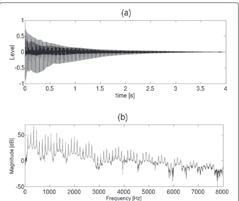
Clavinet tones are known for their sharp attacks and release times, which make the instrument suitable for rhythmic music genres. This is evident upon examination of the signal in the time domain. The attack is sharp as in most struck chordophone instruments, and the release time, similarly, is short, at least with an instrument in mint condition, with an effective yarn damper. The sustain, on the other hand, is prolonged, at least for low and mid tones, as there is minimal energy transfer to the rest of the instrument (in comparison with, say, the piano). Dur-ing sustain, beyond minimal interaction with the magnetic transducer and radiation from the string itself, the only transfer of energy occurs at the string ends, which are con-nected to a metal bar at the far end and the tangent rubber tip at the near end. During sustain, the time required for the sound level to decay by 60 dB (T60) can be as long as 20 s or more. Mid to high tones have a shorter sustain as is typical of stringed instruments. Figure 3 illustrates the time and frequency plot of a A2 tone.

2.3.1 Attack and release transient

Properties of the time-domain displacement wave and the excitation mechanism will be inferred by assuming the pickups to be time-differentiating devices [27].

The attack signals show a major difference between low to mid tones and high tones, as shown in Figure 4. Figure 4b shows the first period of a D3 tone, illustrating a clear positive pulse, reflections, and higher frequency oscillations, while in Figure 4a, the first period of an A4 tone has a clear periodicity and a smooth waveshape.

Figure 3Plot of (a) an A2 tone (116.5 Hz) and (b) its spectral content up to 8 kHz.Please note that the spectrum in(b)is recorded from a pickup signal, hence exhibits the effects of the pickups (clearly visible as a comb pattern with notches at every5th partial) and the amplifier.

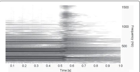
When the key is released, the speaking and nonspeaking parts of the string are unified, giving rise to a change in pitch of short duration, caused by the yarn damper. Given the geometry of the instrument, the pitch decrease after release is three semitones for the whole keyboard. A spec-trogram of the tone before and after release is shown in Figure 5.

2.3.2 Inharmonicity of the string

Another perceptually important feature of a string sound is the inharmonicity [29], due to the lightly dispersive

(4)

Figure 5Spectrogram of the tone before and after key release.

The key release instant is located at 0.5 s.

character of wave propagation in strings. Several meth-ods exist for inharmonicity estimation [30]. In order to quantify the effect of string dispersion, the inharmonicity coefficientBmust be estimated for the whole instrument range. Although theoretically the exact pitch of the par-tials should be related only to the fundamental frequency and theBcoefficient [31] by the following equation:

fn=nf0

(1+Bn2₎_, ₍₁₎

wherefn is the frequency of thenth partial andf0is the fundamental frequency, empirical analysis of real tones shows a slight deviation between the measured partial frequency and the theoretical fn, and thus, a deviation

valueBncan be calculated for each partial related to the

fundamental frequency by the following:

Bn=

f_n2−n2f₀2 n4_f2

0

, (2)

obtained by reworking Equation 1 and replacing the over-allBwith a separateBnfor everynth partial. For practical

use, a number ofBnvalues measured from the same tone

are combined to obtain an estimate of the overall inhar-monicity. A way to obtain this estimate is to use a criterion based on the loudness of the firstNpartials (excluding the fundamental frequency), as described below.

The partial frequencies are evaluated by the use of a high-resolution fast Fourier transform (FFT) on a small segment of the recorded tone. The FFT coefficients are interpolated to obtain a more precise location of par-tial peaks at low frequencies. The peaks are automatically retrieved by a maximum finding algorithm at the neigh-borhood of the expected partial locations for the first N partials and their magnitudes (in dB) are also mea-sured. The fundamental frequency and its magnitude are estimated as well. The Bn coefficients are estimated for

each of theN partials using the measured value forf0to take a possible slight detuning into account. For a per-ceptually motivated Bestimate, theBn estimated values

are averaged with a weighting according to their relative amplitude.

TheBcoefficient has been estimated for eight Clavinet tones spanning the whole key range by evaluating theBn

coefficients forN = 6, i.e., using all the partials from the second to the seventh. Linear interpolation has been used for the remaining keys. The estimate of theBcoefficient for the whole keyboard is shown in Figure 6 and plotted against inharmonicity audibility thresholds as reported in [29]. From this comparison, it is clear that inharmonicity in the low keyboard range exceeds the audibility threshold and its confidence curve, meaning that its effect should be clearly audible by any average listener. For high notes, the inharmonicity crosses this threshold, making it unnotice-able to the average listener, and hence may be excluded from the computational model.

2.3.3 Fundamental frequency

The fundamental frequency is very stable over time. A method based on windowed autocorrelation analysis [32] was used in order to obtain a good estimate off0histories for the attack and sustain phase of the tone. The analysis shows a slight change in time of the pitch, which, however, is perceptually insignificant, with a variation of at most 1 to 2 cents, while audibility thresholds are usually much higher [33].

2.3.4 Higher partials

The spectrum in Figure 3b shows the first harmonics up to 8 kHz for an A2 tone and is quite representative of the spectral profile for many of the Clavinet tones. The second partial always has a magnitude more than 3 dB higher than the first, and often (as in the figure) the third is higher than the second. The spectral envelope of

Figure 6EstimatedBcoefficient for the whole keyboard.

(5)

Clavinet tones shows several peaks and notches due to the superposition of several effects including partial beat-ing (which generates time-varybeat-ing peaks and notches), the pickup position (which applies a comb pattern, later discussed in Section 2.3.5), and amplifier and filter fre-quency responses (discussed in Section 2.3.6). Figure 3b reveals a comb-like pattern given by the pickup position at approximately 544 Hz and multiple frequencies.

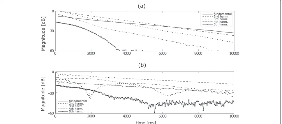
The temporal evolution of partials has been studied. The partials’ decay is usually linear on the decibel scale but sometimes shows an oscillating behavior, i.e., a beating, as seen at the bottom of Figure 7.

The connection between the pitch or key velocity and this phenomenon is still not understood. Data show that the phenomenon stops occurring with keys higher than E4, while the magnitude of the oscillations can be as high as 15 dB peak-to-peak, at frequencies between 0.5 and 2 Hz. The phenomenon does not always noticeably occur, and its amplitude and frequency change from time to time. There is a slight correlation with the key veloc-ity, suggesting that the phenomenon may be correlated to acoustical nonlinearities (e.g., string termination yield-ing), similar to those appearing in other instruments such as the kantele [4]. Generally, when the beating occurs, it is shown in both microphone and pickup recordings. In principle, however, electrical nonlinearities may as well imply some beating between the slightly inharmonic tone partials and harmonics generated by the nonlinearity.

Besides occasional beating, most partials exhibit a monotone decay. For those tones that do not show par-tials beating,T60have been measured separately for each partial. The lowest two to four partials usually show

remarkably longerT60than the higher ones.T60decreases with increasing partial number. However, for most tones, the envelope for partialsT60is not regular but shows an oscillating orripplybehavior, i.e., a fluctuation of theT60 with an approximate periodicity between two and three times the fundamental frequency. Figure 8 shows partials T60 extracted from an E4 tone (vertical lines), compared to the ones from the synthesis model later described in Section 3.

2.3.5 The pickups

Coil pickups, such as those used in guitars, have been studied thoroughly in [26]. The effect of their position is that of linear filtering. Comb-like patterns can be observed in guitar tones and in Clavinet tones due to the reflection of the signal at the string termination. Pick-ups also have their own frequency response given by their electric impedance and the input impedance they are con-nected to [34]. Finally, the relation between the string displacement and the voltage generated by the pickup induction mechanism is nonlinear due to factors such as the nonlinear decay law of the magnetic dipole field. The frequency response of the displacement to voltage ratio is that of a perfect derivative. All the effects listed hereby have been analyzed and modeled.

Details on the comb parameter extraction will be given in Section 3.3 relative to its implementation. The elec-trical impedance Z(ω) of a Clavinet pickup has been measured as described in [34] and is shown in Figure 9. The frequency response of the pickup (proportional to the inverse ofZ(ω)) is almost flat, with differences between maximum and minimum values smaller than 1 dB. The

(6)

Figure 8PartialsT60extracted from an E4 tone compared to the

ones from the synthesis model.PartialsT60for a measured Clavinet

E4 tone (vertical lines) plotted against the partialsT60of an E4 tone

synthesized by the computational model (the dotted line represents the loss filter only, and the dashed line represents the loss filter together with the ripple filter). TheT60values for the first two partials

have been matched with the ripple filter.

impedance can be, in general, greatly modified by the parasitic capacitance present in the connection to the amplifier (e.g., in guitar cables [34]). This parameter has not been evaluated and is considered hereby negligible as the Clavinet has a short connection to the amplifier made partly of shielded cables and partly of copper paths on a printed circuit board.

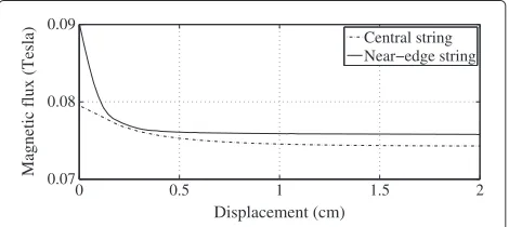
Nonlinearities in the displacement to voltage ratio have been evaluated by means of a software simulation in Vizimag, a commercial electromagnetic simulator. Simu-lations have been carried out for different string gauges, string to pickup distance, and horizontal position of the string with respect to the pickup. The vibration in the horizontal and vertical polarizations has been measured separately, resulting in a negligible voltage generated by the horizontal displacement (25 dB lower than the vertical displacement). The string oscillation was 1 mm peak-to-peak wide, which is the maximum measured oscillation amplitude. The simulations are detailed in [21].

Figure 9Impedance magnitude of the Clavinet pickup versus frequency.

Simulations show that the magnetic flux variation in response to vertical displacement has a negative expo-nential shape (Figure 10), in accord to previous works [26,27,35].

2.3.6 Amplifier and tone controls

Pickup signals are fed to the amplifier section, which also includes tone controls and a volume potentiometer. The amplifier schematic is publicly available [36], and it has been used to gather a basic understanding of its function-ing. Some of the components, such as the tone controls and the transistors, have been isolated to conduct simula-tions and obtain an estimate of the frequency response by means of an electric circuit simulator.

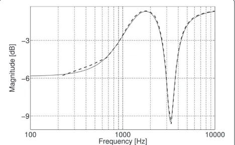
Figure 11 shows simulations for the magnitude fre-quency response of the tone switches, with all the tone switches active (open switches) and with one switch active at a time. Further circuit simulations with the tone stack removed show the amplifier frequency response to be close to flat, with a mild low-shelf (−3 dB at 130 Hz) and high-shelf (+3 dB at 4,000 Hz) characteristic. The tone controls, consisting of first- or second-order discrete fil-ters, have been emulated by digital filters with the transfer function derived from the respective impedance in the analog domain, as detailed in Section 3.4.

3 Computational model

The basic Clavinet string model was presented first in [37] and described in [20]. It consists of a digital waveguide loop structure [38] in which a fractional delay filter [39], a loss filter [40], a ripple filter [41], and a dispersion filter [42] are cascaded. This structure is fed by an attack excita-tion signal, generated on-line by a signal model dependent on an estimate of the virtual tangent velocity. Further-more, the note decay is modeled by increasing the length of the delay line and increasing losses, i.e., decreasing loop gain. The string model is completed by several beating equalizers [43] modulating the gain of the first partials.

More details of this model will now be described.

0 0.5 1 1.5 2

0.07 0.08 0.09

Displacement (cm)

Magnetic flux (Tesla)

Central string Near−edge string

(7)

Figure 11SPICE simulation of the tone switches.All switches active (solid line), soft-only active (dotted line), medium-only active (dashed line), treble-only active (dash-dotted line), brilliant-only active (dash-dot-dot line).

3.1 String model

The Clavinet pitch is very stable during the sustain phase of the tone, and thus, there is no need for change in the overall DWG delay during sustain. Partial decay time anal-ysis from Clavinet tones reveals ripply T60 also shown by microphone-recorded tones. This can be easily repro-duced by the use of a so-calledripple filter, which has been used for the emulation of other instruments as well, such as the harpsichord [41] and the piano [44].

The ripple filter adds a feedforward path with unity gain (which can be incorporated into the delay line) and adds a small amount of the direct signal to it with gainr. The analytic expression is the following:

y[n]=rx[n]+x[n−R] , (3)

wherer is a small coefficient andRis the length of the delayed path length introduced by this filter. The effect of the ripple filter is shown in Figure 8 compared to theT60 of a real tone. The gain at different partials or, conversely, the T60 values are different from one another, enabling the emulation of the real tone behavior seen in Figure 8. Although from a visual inspection of the figures the fit between real and synthesized data may not seem close, from a perceptual standpoint, it must be noted that differ-ences of several seconds in theT60 times, i.e., of several decibels in the magnitude response for a given partial, do not result in a perceivable change, as they fall beneath audibility thresholds, as shown in [45] for the magnitude response of a loss filter in a DWG model.

By increasing or decreasing thercoefficient, the ripple effect is increased or decreased; by changingR, the width of the ripples is changed.Ris in turn calculated from the parameterRratefrom the following:

R=round(RrateLS), (4)

and thus, the total delay line LS is now split into two

sections of lengthRandL =LS−R. To maintain closed

loop stability, the overall gain must be kept below unity, i.e.,g+ |r|<1, withgbeing the loss filter gain.

The ripple filter coefficients can be adjusted in order to match those observed in recorded tones. The ripple parameters in Figure 8, for instance, areRrate = 1/2 and r= −0.006. In the model,Rrateandrare randomly chosen at each keystroke respectively in the range between 1/2 to 1/3 and−0.006 to−0.001, according to observations.

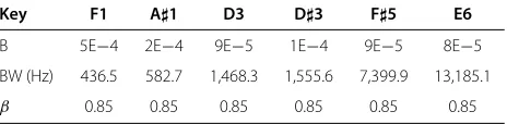
The design of the dispersion filter follows the algorithm described in [46]a. The algorithm achieves the desiredB coefficient in a frequency band specified by the user. The authors suggest that this be at least 10 times the fun-damental frequency. The B coefficients, the bandwidth (BW), and theβparameters used for every key are linearly interpolated from the values in Table 1.

The Clavinet tones may contain beating partials as shown in Figure 7. An efficient and easily tunable method to emulate this is to cascade a so-calledbeating equalizer, proposed in [43] with the DWG loop.

The beating equalizer is based on the Regalia-Mitra tun-able filters [47] but adds a modulating gain at the output stageK[n], wherenis the time index.

In brief, such a device is a band-pass filter with vary-ing gain at the resonatvary-ing frequency. The gain can vary according to an arbitrary function of time, but for the emulation of Clavinet tones, it has been decided to use a|cos(2πfn)|law, which well approximates the behavior seen in Figure 7 in Section 2.3.4. The modulated gain is the following:

K[n]=10|cos(202πfn)|_. ₍₅₎

In order to modulateMpartials,Mbeating equalizers are needed. It was shown, however, by informal listening tests that it is difficult to perceive the effect of more than three beating equalizers working at the same time.

The computational cost of this device is low, consisting of a biquad filter plus the overhead of five operations per sample (three additions and two multiplications, as can be seen in [43] and Figure 2).

Table 1Bcoefficients used for the design of the dispersion filter

Key F1 A1 D3 D3 F5 E6

B 5E−4 2E−4 9E−5 1E−4 9E−5 8E−5

BW (Hz) 436.5 582.7 1,468.3 1,555.6 7,399.9 13,185.1

(8)

3.2 Excitation model

The string model described so far can be fed at attack time with an excitation signal of some kind. In the pro-posed model, the excitation signal consists of a smooth pulse similar to those seen in low- to mid-range tones. The pulse is made by joining an attack ramp with its reverse. The ramp is obtained by fitting the following polynomial to some pulses extracted from recorded tones:

f(x)=aPxP+aP−1xP−1+...+a1x+a0. (6) The polynomial coefficients were calculated from sev-eral least square error fits to some portions of sig-nals extracted from the recordings. These sigsig-nals have a smooth triangular shape and represent the pickup out-put from the tangent hitting the string. A polynomial has been obtained with order P = 6 and coefficients in descending order: −2.69E−8, 2.53E−6, −9.54E−5, 1.74E−3,−1.44E−2, 4.50E−2,−3.50E−2. This signal is scaled by a gain and stretched by interpolation accord-ing to the player dynamic, makaccord-ing it shorter or longer. To calculate the pulse length in samplesN, the average key velocityvand the initial distancedbetween the tangent and stud are required; thus,

N= fsd

v , (7)

wherefsis the sampling frequency. The average key veloc-ity normally varies linearly in the range 1 to 4 m/s and is mapped to integers from 1 to 127, as per the Musical Instrument Digital Interface (MIDI) standard. Figure 12 showspianoandforteexcitation signals calculated with our method.

The pulse signals seen in Clavinet tones have a smooth triangular shape and represent the pickup output from the tangent hitting the string. Most of the recorded tones exhibit a similar pulse at the beginning of the tone, hence making this a good approximation for the string excita-tion produced by the tangent in most cases. Because the signal extracted from the pickups is the time derivative of the string displacement at the pickup position, when using

Figure 12Excitation pulse signals for piano and forte tones.

its approximation as an excitation, it must be ensured that the wave variables in the digital waveguide are also time-differentiated approximations of the displacement of the Clavinet string. This allows differentiation to be avoided when emulating the effect of pickups if these are linear devices. With nonlinear pickups (as it is the case), integration must be performed before the nonlinear stage.

3.3 Model for pickups

The proposed pickup model includes a comb effect dependent on the pickup position, the magnetic field dis-tance nonlinearity, and the emulation of the pickup selec-tor switches. The traveling waves reflected at the string termination are transduced by the pickups, thus creating a comb characteristic in frequency. This effect can be emu-lated by a comb filter with negative gain (ideally−1 for a stiff string) and a delay equal to the time needed for the wave to propagate from the pickup position to the string termination and back [26]. As discussed in Section 2.3.5, string dispersion also affects the position of the comb notches. In [48], the amount of dispersion is shown to be equal to the string inharmonicity itself. A duplicate of the dispersion filter used in the string model could be added to the comb feedforward path to obtain this sec-ondary effect. However, to achieve a trade-off between computational efficiency and sound quality, the duplicate filter has not been implemented as it would increase the computational cost by 25%.

The comb filter needs two parameters to be calculated: the delay in samples and the gain. The latter has been set to −1 for both the pickups as the string termination is assumed to only invert the incoming wave. The former can be calculated with a simple proportion after a direct measure of the pickup’s distance from the string termina-tion: the physical string length to pickup distance ratio can be multiplied to the total delay line lengthLtarg.

The overall frequency response has not been modeled being perceptually flat (as discussed in Section 2.3.5).

The pickup nonlinearity reported in Section 2.3.5 can be implemented as an exponential or an N th-order polynomial. The latter has a lower computational cost, and it can be computed on modern DSP archi-tectures with N − 1 consecutive multiply-accumulate operations and N products following Horner’s method [49]. The polynomial coefficients used are reported in Table 2.

(9)

Table 2 Pickup polynomial coefficients

Since the excitation is a velocity wave and the nonlin-earity applies to a displacement wave, the signal must be integrated before the nonlinearity. For real-time scenarios, a leaky integrator can be used as the one proposed in [50]. Afterwards the nonlinear block differentiation must be applied to emulate that performed by pickups [27]. A sim-ple first-order digital differentiator as in [51] is sufficient and suited for real-time operation.

3.4 Model for the amplifier

Analyses from Section 2.3.6 suggested that the amplifier and the tone switch frequency response can be mod-eled in the digital domain with simple infinite impulse response (IIR) digital filters, keeping the computational cost low. The tone stack consists of four first- or second-order filters which can be bypassed by a switch. Details about the filters are provided in Table 3. For emulation in the digital domain, the impedanceZi(s) is calculated

for each filter in the Laplace domain and then trans-formed by bilinear transform in a digital transfer func-tionHi(z). The parallelZi(s) in the analog domain can

hence be emulated by cascading the Hi(z) filters in the

digital domain.

Figure 13Comparison of the exponential fit to the simulated data and the polynomial fit.Magnetic flux variation against vertical string displacement for a string passing over the center of the pickup (marker), an exponential fit (dashed line), and a fourth-degree polynomial approximation (solid line).

Table 3 Filter transfer functions

Filter Components Zi(s) Hi(z)

As an example, 14 compares one of the tone switch combinations and its digital filter implementation.

Finally, the frequency response of the amplifier exclud-ing the tone stack is emulated with digital shelf filters corresponding to the data provided in Section 2.3.6. A reliable estimate of the nonlinearity introduced by the transistors was not possible as a faithful transistor model was not available for the specific transistor models in the computer software used during tone switch simulations. The transistor nonlinearities [52] have been measured on a real Clavinet by the use of a tone generator and a sig-nal asig-nalyzer. The input sigsig-nal was a sine wave at 1 kHz of amplitude equal to the maximum one generated by pick-ups with normal polyphonic playing (400 mV) showing a total harmonic distortion (THD) of 1% with normal poly-phonic playing, rising to 3.6% for the highest peaks during fortissimochord playing, which, however, is obtained only very rarely. Considering the 1% THD data as the upper bound for normal playing, the nonlinear character of the

(10)

amplifier has been neglected, considering that the gen-erated harmonic content is likely to be masked by the Clavinet tones.

3.5 Tangent knock

A secondary feature of the Clavinet sound is the pres-ence of a knock sound, due to the tangent hitting the stud and hence the soundboard. The presence of this knocking sound in the pickup recordings may seem curi-ous, but it can easily be explained by the fact that the impact of the tangent with the soundboard stud involves the string which is placed between the two bodies and in contact with the soundboard and hence transmits part of the sound (including the modal resonances of the sound-board) through to the pickups.

This knocking sound is clearly audible in high tones, where its overlap with the tone harmonics is lower. In order to partially model this knock, a sample of this sound has been extracted from an E6 tone, where the funda-mental frequency lies over 1,300 Hz. The knocking sound, which has most of its energy concentrated below 1,200 Hz, can be isolated by filtering out everything over the tone fundamental frequency.

In the proposed model, a triggered sample is used. The sample is the same for any key (the secondary impor-tance of this element does not give a strong motivation for precise modeling). Additionally, a mild low-pass fil-ter can be added with a slightly random cutoff frequency for each note triggering in order to reduce the sample repetitiveness.

3.6 Overview of the complete model and computational cost

The computational model described so far has been first implemented in Matlab®_{. The target of this work has} been the development of a low-complexity model that

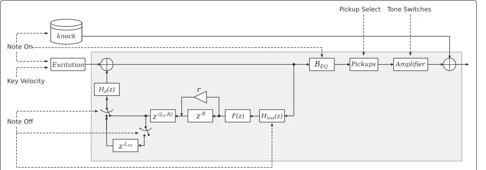
could fit a real-time computing platform; thus, the port-ing of that model did not require any particular change in structure for the subsequent real-time implementation. The computational model described so far, depicted in Figure 15, stands for both the Matlab and the real-time implementation.

To summarize the work done to build this model, an overview of the basic blocks will be given. The DWG model consists of the delay line, which is split into two sections (z−(LS−R)_and_z−R_{) in order to add the ripple}

fil-ter. The DWG loop includes the one-pole loss filter [53] Htarg(z) which adds frequency-dependent damping and the dispersion filterHd(z)which adds the inharmonicity

characteristic to metal strings. The fractional delay filter F(z)accounts for the fractional part ofLSwhich cannot be

reproduced by the delay line.

While the Clavinet pitch during sustain is very stable, and thus there is no need for changing the delay length, a secondary delay line, representing the nonspeaking part of the string, is needed to model the pitch drop at release. This delay line z−LNS _{is connected to the DWG loop at}

release time to model the key release mechanism. To excite the DWG loop, there is the excitation gen-erator block, named Excitation, which makes use of an algorithm described in [20] to generate the an excitation signal related to key velocity and data on the tangent to string distance. This is triggered just once at attack time.

Several blocks are cascaded in the DWG loop. The beat-ing equalizer (BEQ), composed of a cascade of selective bandpass filters with modulated gain, emulates the beat-ing of the partial harmonics and completes the strbeat-ing model. Then, thePickupblock emulates the effect of pick-ups, while theAmplifieremulates the amplifier frequency response, including the effect of the tone switches.

Finally, the soundboard knocksample is triggered at a ‘note on’ event to reproduce that feature of the Clavinet

(11)

tone. This is similar to what has been done for the emula-tion of the clavichord [23], an instrument that shows some similarities with the Clavinet.

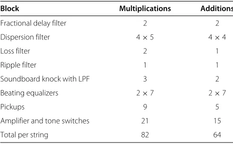
The theoretical computational cost of the complete model can be estimated for the worst case conditions and is reported in Table 4. The worst case conditions occur for the lowest tone (F1), which needs the longest delay line and the highest order for the dispersion filter. The latter depends on the estimate of theBcoefficients made during the analysis phase and the parameters used to design the filter. With the current data, the maximum order of the dispersion filter is eight.

The memory consumption is mostly due to the delay lines, which, at a 44,100-Hz sampling frequency, require at most 923 samples (a longer delay line is not required as the dispersion filter takes into account a part of the loop delay), which, together with the taps required by comb filters, can amount to approximately 1,000 samples of memory per string.

4 Real-time implementation

The model discussed in Section 3 is well suited to a real-time implementation, given its low computational cost. The implementation has been performed on the Pure Data (PD) open-source software platform, a graphical programming language [54].

Some technical details regarding the PD patch imple-mentation will be now discussed.

The main panel includes real-time controllable parame-ters such as pickup selector, tone switches, yarn damping, ripple filter coefficients, soundboard knock volume, beat-ing equalizers settbeat-ings, and the master volume.

The delay line used for digital waveguide modeling is allocated and written by the [delwrite∼] object and is read by the[vd∼]object. The latter also imple-ments the fractional delay filter with a four-point inter-polation algorithm.

Table 4 Computational cost of the Clavinet model per sample per string

Block Multiplications Additions

Fractional delay filter 2 2

Dispersion filter 4×5 4×4

Loss filter 2 1

Ripple filter 1 1

Soundboard knock with LPF 3 2

Beating equalizers 2_×7 2_×7

Pickups 9 5

Amplifier and tone switches 21 15

Total per string 82 64

Total FLOPS per string is 6.4 MFLOPS at 44,100 Hz.

The dispersion filter is made of cascaded second-order sections (SOSs). These are not easily dynamically allo-cated at runtime in the PD patching system; hence, a total of four SOSs has been preallocated and coefficients have been prepared in Matlab. More than four SOSs would be needed for the lowest tones if a more accurate emulation of the dispersion were desired (which can be achieved by increasing the frequency cutoff of the mask in the dispersion filter design algorithm), but a trade-off between computational cost and quality of sound has been made.

The PD patchb for the Clavinet has been created and tested on an embedded GNU/Linux platform running Jack as the real-time audio server at a sampling fre-quency of 44,100 Hz. The platform is the BeagleBoard, a Texas Instruments OMAP-based solution (Dallas, TX, USA), with an ARM-v8 core (equipped with a floating point instruction set), running a stripped-down version of Ubuntu 10.10 with no desktop environment [55]. A test patch with 10 instances of the string model and the amplifier requires an average 97% CPU load, leaving the bare minimum for the other processes to run (includ-ingpd-guiand system services) but causing no Xruns (i.e., buffer over/underruns). The current PD implementa-tion of the model only relies on the PD-extended package externals: this means that, in the future, if using custom-written C code to implement parts of the algorithm (e.g., the whole feedback loop), the overhead for the computa-tional cost can be highly reduced. This will gain headroom for additional complexity in the model. The audio server guarantees a 5.8-ms latency (128 samples at 44,100 Hz), thus unnoticeable when the patch is played with a USB MIDI keyboard.

5 Model validation

A preliminary model validation has been done by compar-ing real data with synthetic tones. Throughout the paper, some differences have been shown in the string frequency response (Figure 8) and in the frequency response of the amplifier tone control (Figure 16). Furthermore, the time and spectral plot of a tone synthesized by the model (to be compared to the sampled counterpart in Figure 3) is shown in Figure 16.

A more detailed comparison between the former two tones is shown in Figure 17, where the partial envelope has been extracted, smoothed, and compared. Although the two spectra do not exactly match, from a perceptual standpoint, the differences are of minor importance.

(12)

Figure 16Plot of (a) a synthesized A2 tone and (b) its spectral content up to 8 kHz.

model described in [20]. Test results conducted on the present model show slight differences with the ones pre-sented in [22], which will be briefly reported for the sake of completeness.

The metric used to evaluate the results is called accu-racy or discrimination factor [56],d, which is defined as follows:

d= PCS−PFP+1

2 , (8)

where PCS and PFP are the correctly detected synthetic percentage and falsely identified synthetic percentage (recorded samples misidentified as synthetic), respec-tively. A discrimination factor of 100% represents perfect

Figure 17Comparison of the partial envelope of real (77.78 Hz) and synthesized D2 tones up to 4 kHz.Thin solid line, real; thick dashed line, synthesized. The partial locations are given by the gray stem plot.

distinguishability for the recorded and synthetic tones, whereas 50% represents random guessing. In previous works, a threshold of 75% has been accepted as the bor-derline, under which the sound can be considered not distinguishable [56-58]; however, in this work, the 75% threshold will be called a likelihood threshold, under which the sound can be considered very close to the real one. Perfect indistinguishability coincides with random guessing.

The listening tests show a good level of realism as the threshold of 75% for the discrimination averaged among the subjects is never reached. The d factor averaged among the various subject categories is 53%. Musicians with knowledge of the Clavinet sound obtained the high-est d score, 58%, 3% lower than that obtained with the previous model, showing an increase in sound quality with the current model. Tests have been performed with both single tones and melodies.

6 Conclusions and future work

This paper describes a complete digital waveguide model for the emulation of the Clavinet, including detailed acoustical analysis and parametrization and modeling of pickups and the amplifier. Important issues related to the analysis of the recordings, the peculiarity of the tan-gent mechanism, and the way to reproduce the amplifier stage are addressed. Specifically, the excitation wave-form is generated depending on the key strike veloc-ity, and the release mechanism is modeled from the speaking and nonspeaking string lengths. The frequency response of the pickups based on impedance measure-ment on a Clavinet pickup is discussed, while the ampli-fier model is based on digital filters derived from circuit analysis and is compared to computer-aided electrical simulations.

A real-time Pure Data patch is described that can run several string instances on a common PC, allowing for at least 10-voice polyphony. Subjective listening tests are briefly reported to prove a good degree of faithfulness of the model to the real Clavinet sound. Future work on the model includes a mixed FDTD-DWG model [59] to introduce nonlinear interaction in the tangent mechanism while keeping the computational cost low. The listen-ing tests reported in this paper stand as one of the first attempts in subjective evaluation for musical instrument emulation, and, even revealing its usefulness on purpose, more advanced methods and metrics will be explored in the future.

Endnotes

(13)

b _{The PD patch and sound samples of the}

computational model will be shared with the community and made available at http://a3lab.dii.univpm.it/projects/ jasp-clavinet.

Competing interests

The authors declare that they have no competing interests.

Acknowledgements

Many thanks to Emanuele Principi, PhD, from the Università Politecnica delle Marche Department of Information Engineering, for the development of the software platform used for the tests, called A3Lab Evaluation Tool. One of the authors (Bilbao) was supported by the European Research Council, under grant StG-2011-279068-NESS.

Author details

1_{Department of Information Engineering, Università Politecnica delle Marche,}

Via Brecce Bianche 12, Ancona 60131, Italy.2_{Department of Signal Processing}

and Acoustics, Aalto University, Otakaari 5, 02015, Finland.3_{Department of}

Music, University of Edinburgh, King’s Buildings, Mayfield Rd., Edinburgh EH9 3JZ, UK.

Received: 15 March 2012 Accepted: 5 April 2013 Published: 13 May 2013

References

1. G De Sanctis, A Sarti, Virtual analog modeling in the wave-digital domain. IEEE Trans. Audio Speech Lang. Process.18(4), 715–727 (2010) 2. T Hélie, Volterra series and state transformation for real-time simulations

of audio circuits including saturations: application to the Moog ladder filter. IEEE Trans. Audio Speech Lang. Process.18(4), 747–759 (2010) 3. F Fontana, M Civolani, Modeling of the EMS VCS3 voltage-controlled filter

as a nonlinear filter network. IEEE Trans. Audio Speech Lang. Process. 18(4), 760–772 (2010)

4. C Erkut, M Karjalainen, P Huang, V Välimäki, Acoustical analysis and model-based sound synthesis of the kantele. J. Acoust. Soc. Am.112(4), 1681–1691 (2002)

5. H Penttinen, J Pakarinen, V Välimäki, M Laurson, H Li, M Leman, Model-based sound synthesis of the guqin. J. Acoust. Soc. Am.120, 4052–4063 (2006)

6. SJ Cho, U Chong, S Cho, BSynthesis of the Dan Tranh based on a parameter extraction system. J. Audio Eng. Soc.58(6), 498–507 (2010) 7. M Vail,Vintage Synthesizers, 2nd edn. (Miller Freeman Books, San

Francisco, 2000)

8. JO Smith, Physical Audio Signal Processing for Virtual Musical Instruments and Digital Audio Effects. http://www.w3k.org/books/. Accessed 19 Aug 2011

9. V Välimäki, J Pakarinen, C Erkut, M Karjalainen, Discrete-time modelling of musical instruments. Reports on Prog. Phys.69, 1–78 (2006)

10. S Bilbao,Numerical Sound Synthesis: Finite Difference Schemes and Simulation in Musical Acoustics. (Wiley, Chichester, 2009)

11. L Trautmann, R Rabenstein,Digital Sound Synthesis by Physical Modeling Using the Functional Transformation Method. (Kluwer/Plenum, New York, 2003)

12. A Chaigne, A Askenfelt, Numerical simulations of piano strings. a physical model for a struck string using finite difference methods. J. Acoust. Soc. Am.95(2), 1112–1118 (1994)

13. B Bank, L Sujbert, Generation of longitudinal vibrations in piano strings: from physics to sound synthesis. J. Acoust Soc. Am.117(4), 2268–2278 (2005)

14. B Bank, S Zambon, F Fontana, A modal-based real-time piano synthesizer. IEEE Trans. Audio Speech Lang. Process.18(4), 809–821 (2010)

15. N Lee, JO Smith, V Välimäki, Analysis and synthesis of coupled vibrating strings using a hybrid modal-waveguide synthesis model. IEEE Trans. Audio Speech Lang. Process.18(4), 833–842 (2010)

16. V Välimäki, J Huopaniemi, M Karjalainen, Z Jánosy, Physical modeling of plucked string instruments with application to real-time sound synthesis. J. Audio Eng. Soc.44, 331–353 (1996)

17. J Bensa, S Bilbao, R Kronland-Martinet, J Smith III, The simulation of piano string vibration: from physical models to finite difference schemes and digital waveguides. J. Acoust. Soc. Am.114, 1095–1107 (2003) 18. J Rauhala, HM Lehtonen, V Välimäki, Toward next-generation digital

keyboard instruments. IEEE Signal Process. Mag.24(2), 12–20 (2007) 19. S Bilbao, M Rath, in128th AES Convention. Time domain emulation of the

Clavinet (London, 22–25 May 2010), p. 7

20. L Gabrielli, V Välimäki, S Bilbao, inProceedings of the International Computer Music Conference. Real-time emulation of the Clavinet (Huddersfield, 31 July–5 Aug 2011), pp. 249–252

21. L Remaggi, L Gabrielli, R de Paiva, V Välimäki, S Squartini, inDigital Audio Effects Conference 2012 (DAFx-12). A pickup model for the clavinet ((York, 17–21 Sept 2012)

22. L Gabrielli, S Squartini, V Välimäki, in131st AES Convention. A subjective validation method for musical instrument emulation (New York, 20–23 Oct 2011)

23. V Välimäki, M Laurson, C Erkut, Commuted waveguide synthesis of the clavichord. Comput. Music J.27(1), 71–82 (2003)

24. C d’Alessandro, On the dynamics of the clavichord: from tangent motion to sound. J. Acoust. Soc. Am.128, 2173–2181 (2010)

25. Pianoteq CL1. http://www.pianoteq.com/commercial%5Faddons. Acceseed 19 Aug 2011

26. RC de Paiva, J Pakarinen, V Välimäki, Acoustics and modeling of pickups. J. Audio Engineering Soc.60(10), 768–782 (2012)

27. N Horton, T Moore, Modeling the magnetic pickup of an electric guitar. Am. J. Phys.77, 144–150 (2009)

28. A Nackaerts, B De Moor, R Lauwereins, inProceedings of the International Computer Music Conference. Measurement of guitar string coupling (Goteborg, 16–21 Sept 2002), pp. 321–324

29. H Järveläinen, V Välimäki, M Karjalainen, Audibility of the timbral effects of inharmonicity in stringed instrument tones. Acoust. Res. Lett. Online, ASA. 2(3), 79–84 (2001)

30. J Rauhala, H Lehtonen, V Välimäki, Fast automatic inharmonicity estimation algorithm. J. Acoust. Soc. Am.121(5), 184–189 (2007) 31. H Fletcher, E Blackham, R Straton, Quality of piano tones. J. Acoust. Soc.

Am.34(6), 749–761 (1962)

32. LR Rabiner, On the use of autocorrelation analysis for pitch detection. IEEE Trans. Acoust. Speech Signal Process.25(1), 24–33 (1977)

33. H Järveläinen, V Välimäki, inProceedings of the International Computer Music Conference. Audibility of initial pitch glides in string instrument sounds (Havana, 17–23 Sept 2001), pp. 282–285

34. C De Paiva, H Penttinen, in131st AES Convention. Cable matters: instrument cables affect the frequency response of electric guitars (New York, 20–23 Oct 2011)

35. G Lemarquand, V Lemarquand, Calculation method of

permanent-magnet pickups for electric guitars. IEEE Trans. Magnetics. 43(9), 3573–3578 (2007)

36. www.clavinet.com. Clavinet D6 amplifier schematic. http://www.gti.net/ junebug/clavinet/Clavinet%5FD6%Fschematic.pdf. Accessed 19 Aug 2011

37. L Gabrielli, Modeling of the clavinet using digital waveguide synthesis techniques. M.Sc. thesis, Università Politecnica delle Marche, 2011 38. DA Jaffe, JO Smith, Extensions of the Karplus-Strong plucked-string

algorithm. Comput. Music J.7(2), 56–69 (1983)

39. T Laakso, V Välimäki, M Karjalainen, U Laine, Splitting the unit delay-tools for fractional delay filter design. IEEE Signal Process. Mag.13(1), 30–60 (1996)

40. B Bank, V Välimäki, Robust loss filter design for digital waveguide synthesis of string tones. IEEE Signal Process. Lett.10(1), 18–20 (2003) 41. V Välimäki, H Penttinen, J Knif, M Laurson, C Erkut, Sound synthesis of the

harpsichord using a computationally efficient physical model. EURASIP J. Appl. Signal Process.7, 934–948 (2004)

42. S Van Duyne, J Smith, inProceedings of the International Computer Music Conference. A simplified approach to modeling dispersion caused by stiffness in strings and plates (Aarhus, 12–17, Sept 1994), pp. 335–343 43. J Rauhala, inDigital Audio Effects Conference (DAFx-07). The beating

(14)

44. J Rauhala, M Laurson, V Välimäki, H Lehtonen, V Norilo, A parametric piano synthesizer. Comput. Music J.32(4), 17–30 (2008)

45. H Järveläinen, T Tolonen, Perceptual tolerances for the decaying parameters in string instrument synthesis. J. Audio Engineering Soc. 49(11), 1049–1059 (2001)

46. JS Abel, V Välimäki, JO Smith, Robust, efficient design of allpass filters for dispersive string sound synthesis. IEEE Signal Process. Lett.17(4), 406–409 (2010)

47. P Regalia, S Mitra, Tunable digital frequency response equalization filters. IEEE Trans. Acoust. Speech Signal Process.35(1), 118–120 (1987) 48. N Lindroos, H Penttinen, V Välimäki, Parametric electric guitar synthesis.

Comput. Music J.35(3), 18–27 (2011)

49. W Horner, A new method of solving numerical equations of all orders, by continuous approximation. Philos. Trans. Royal Soc. London.109, 308–335 (1819)

50. E Brandt, inProceedings of the International Computer Music Conference. Hard sync without aliasing (Havana, 9–14 Sept 2001), pp. 365–368 51. MA Al-Alaoui, Novel digital integrator and differentiator. IEEE Electron.

Lett.29(4), 376–378 (1993)

52. D Yeh, Digital implementation of musical distortion circuits by analysis and simulation. Ph.D. dissertation, Stanford University, 2009. https:// ccrma.stanford.edu/~dtyeh/papers/DavidYehThesissinglesided.pdf. Accessed 8 May 2013

53. B Bank, Physics-based sound synthesis of the piano. Ph.D. dissertation, Helsinki University of Technology, 2000 http://www.acoustics.hut.fi/~ bbank/thesis.html. Accessed 8 May 2013

54. M Puckette, inProceedings of the Second Intercollege Computer Music Concerts. Pure data: another integrated computer music environment (Tachikawa, 7 May 1997), pp. 37–41

55. L Gabrielli, S Squartini, E Principi, F Piazza, inEuropean DSP Education and Research Conference (EDERC 2012). Networked beagleboards for wireless music applications (Amsterdam, 13–14 Sept 2012)

56. CW Wun, A Horner, Perceptual wavetable matching for synthesis of musical instrument tones. J. Audio Engineering Soc.49, 250–262 (2001) 57. S Wun, A Horner, Evaluation of weighted principal-component analysis

matching for wavetable synthesis. J. Audio Engineering Soc.55(9), 762–774 (2007)

58. H Lehtonen, H Penttinen, J Rauhala, V Välimäki, Analysis and modeling of piano sustain-pedal effects. J. Acoust. Soc. Am.122, 1787–1797 (2007) 59. M Karjalainen, C Erkut, Digital waveguides versus finite difference

structures: equivalence and mixed modeling. EURASIP J. Adv. Signal Process.7, 978–989 (2004)

doi:10.1186/1687-6180-2013-103

Cite this article as:Gabrielliet al.:A digital waveguide-based approach for Clavinet modeling and synthesis.EURASIP Journal on Advances in Signal Processing20132013:103.