PhD Dissertation
International Doctorate School in Information and Communication Technologies
DISI - University of Trento
Visual Saliency Detection
and Its Application to Image Retrieval
Oleg Muratov
Advisor:
Assist prof. Giulia Boato
Universit`a degli Studi di Trento
Co-advisor:
Prof. Francesco G. De Natale
Universit`a degli Studi di Trento
Abstract
People perceive any kind of information with different level of attention and involvement. It is due to the way how our brain functions, redundancy and importance of the perceived data. This work deals with visual information, in particular with images. Image analysis and processing is often requires running computationally expensive algorithms. The knowledge of which part of an image is important over other parts allows for reduction of data to be processed. Besides computational cost a broad variety of applications, including image compression, quality assessment, adaptive content display and rendering, can benefit from this kind of information. The development of an accurate visual importance estimation method may bring a useful tool for image processing domain and that is the main goal for this work. In the following two novel approaches to saliency detection are presented. In comparison to previous works in this field the proposed approaches tack-les saliency estimation on the object-wise level. In addition, one of the proposed approach solves saliency detection problem through modelling 3-D spatial relationships between objects in a scene. Moreover, a novel idea of the application of saliency to diversification of image retrieval results is presented.
Keywords
Contents
1 Introduction 1
2 Visual saliency detection 7
2.1 Introduction . . . 7
2.2 State of the art on visual saliency detection . . . 9
2.3 The proposed innovations . . . 21
2.4 Segment-based saliency detection . . . 22
2.5 Depth-based saliency detection . . . 32
2.6 Saliency evaluation dataset . . . 39
2.7 Evaluation . . . 43
3 Diversification of visual content using saliency maps 51 3.1 Introduction . . . 51
3.2 State of the art on diversification in image retrieval . . . . 53
3.3 The proposed approach . . . 55
3.3.1 Visual Features . . . 55
3.3.2 Search Results Diversification . . . 58
3.4 Evaluation . . . 61
4 Conclusion 73
A Saliency detection evaluation 87
List of Tables
2.1 Segmentation parameters . . . 24
2.2 Performance of the proposed methods . . . 44
3.1 Example of an annotation . . . 64
3.2 Experiment 1 results . . . 66
3.3 Experiment 2 results . . . 67
List of Figures
2.1 Saliency detection methods ontology . . . 10
2.2 Segment-based saliency detection scheme . . . 23
2.3 Saliency dependency on colors . . . 25
2.4 Luminance contrast . . . 26
2.5 Center-surround histogram filter . . . 27
2.6 Occlusion feature . . . 29
2.7 Geometric class detector output . . . 30
2.8 Shape descriptor . . . 32
2.9 Depth extraction . . . 33
2.10 Depth estimation example . . . 34
2.11 Spatial closeness . . . 35
2.12 Tangent-like feature output . . . 36
2.13 Depth-based saliency detection scheme . . . 38
2.14 Fixation points over time . . . 40
2.15 Example images from the dataset . . . 41
2.16 Ground-truth collection UI . . . 42
2.17 Features analysis I . . . 46
2.18 Features analysis II . . . 47
2.19 Features analysis III . . . 48
2.20 Evaluation . . . 50
3.1 Feature extraction scheme . . . 57
3.3 Example of coverage measure computation . . . 62
3.4 Coverage measure pace. As it can be seen ranking with saliency allows for faster coverage of a dataset. Also one can notice that after 15 images coverage grows much slower. 65 3.5 Results of re-ranking for faces . . . 69
3.6 Example of re-ranking for category bear . . . 70
3.7 Example of re-ranking for category bear: annotations . . . 71
A.1 Test image: marriage . . . 89
A.2 Test image: laboratory . . . 90
A.3 Test image: church . . . 91
A.4 Test image: astronaut . . . 92
A.5 Test image: lady . . . 93
A.6 Test image: fire-car . . . 94
A.7 Test image: aerial . . . 95
A.8 Test image: dog . . . 96
A.9 Test image: dolphin . . . 97
A.10 Test image: bears . . . 98
B.1 Example of re-ranking for category pyramid . . . 100
B.2 Example of re-ranking for category bridge . . . 101
B.3 Example of re-ranking for category blimp . . . 102
Chapter 1
Introduction
While analysing the content of images and videos one can notice that
im-portance of the content within the frame is not equal. We are living in
the age of information revolution. Information is everywhere in our lives.
Television, radio, newspapers, social networks. This work deals with very
particular part of information - images, mainly photographs. Images may
represent different aspects of our live: everyday routine, events, holiday
trips and arts. Like in any means of information exchange only some parts
of an image contain the desired information. Indeed, due to the way
im-ages are created there is no way of full control over their content. Consider
for example you want to make a picture of some monument in a city. This
monument may be surround by some building, in between the monument’s
face surface and camera plane there could be people passing over,
depend-ing on the orientation of the camera with respect to the monument sky or
ground plane may also appear in the frame. Although it is possible to avoid
these objects by zooming very close to the monument, this is rarely done,
because then the visualization of the monument will be less informative.
Thereby inclusion of two types of content (foreground and background) in
images is inevitable. For instance, in the aforesaid toy example the
CHAPTER 1. INTRODUCTION
background. It is natural to think that the foreground part of an image is
to be perceived as an important peace of information.
The same problem can be viewed from observer’s point of view. Starting
from our eyes the visual information is perceived unequally. The
resolu-tion of retina depend on locaresolu-tion of objects in the visual field. Rays falling
onto the center of the retina are perceived with higher resolution.
Recep-tive fields in the cortex span for over 30 degrees, however their placement is
not uniform at the mass of the fields are located at the center of the gaze.
Each higher perception level of neural network performs a more complex
information and capacity of each level decreases while ascending from
bot-tom to the top. This peculiarities leads to the competition of information
streams. Thus the way how our brain is functioning orders incoming
vi-sual information by its importance. The saccade search and selectivity
process are guided by bottom-up and top-down stimulus. Top-down
stim-ulus usually represent selection based on knowledge, for example, a subject
is looking for a picture of an animal. Bottom-up stimulus are driven by
properties of perceived visual information, such as high contrast, difference
in orientation, etc.
Ability of automatic detection of important regions can be a priceless
tool for a broad variety of multimedia applications. A wide spectrum of
application may benefit from separative processing of important and less
important regions of an image. Thus development of a robust method for
automatic detection of important regions in image may lead to significant
progress in multimedia processing. As it will be shown later there already
exist a number of approaches to automatically determine important
re-gions, or as it is often called saliency. However, as it is will be shown in
Chapter 2 there is still room for improvements in this direction and in this
work two novel approaches to saliency detection are presented.
de-CHAPTER 1. INTRODUCTION
tection were presented, still a few number of works were dedicated to the
application of saliency information for improving multimedia processing
al-gorithms and addressing new challenging problems. Current applications
include gentle advertising in images [37], where a saliency map is used to
insert advertisement above unimportant region of an image, thus
prevent-ing advertisement block from occlusion of foreground object. An approach
to use of saliency detection in image retrieval was presented in [23]. The
authors proposed to use saliency value as a weighting parameter for SIFT
key-points. Thus similarity of two images is defined by number of matched
SIFT key-points only from their salient areas. A similar approach was
pre-sented in [39]. Though instead of using key-points for similarity measure,
features employed in saliency detection are used. A quite similar idea can
be found in [61], where saliency and color features are used for measuring
similarity of images. Another way of using saliency for image retrieval was
presented in [19]. Here, the authors apply saliency to interactive retrieval.
At each iteration feedback from a user is used to construct affinity matrix
that is formed by salient regions of positive images that is further used as
query. Alternative way for the same problem was proposed in [62]. The
authors proposed using saliency information to drive a semantics model of
an image that is further used for retrieval.
Another common application of saliency is adaptive content display.
For instance, in [40] a saliency based image re-targeting approach was
presented. The authors proposed using unimportant regions of images
as areas for continuous seam carving. Thereby, scale compression and
corresponding spatial distortion does not affect important regions of an
image and thus perceptional content of an image is not destroyed. In [42]
the authors proposed using saliency maps for thumbnail generation. A
thumbnail is generated in a way such that a corresponding bounding box
CHAPTER 1. INTRODUCTION
Saliency detection has also found its application in object recognition. For
instance, in [22] saliency is employed for image classification. Here, the
authors targeted categorization of objects in images to classes like bicycles,
bus, cars, etc. Saliency is used to emphasize features in important areas.
As a features several key-points extractors were used. In [48] a survey on
using saliency for object categorization was presented. Here, the authors
proposed to use saliency as one of the feature together with key-points
both during training and classification steps.
Image compression can also benefit from using saliency detection. For
example, in [16] the authors proposed to use saliency as a parameter
defin-ing compression ration of different parts of a frame for MPEG compression.
A similar idea was proposed in [28], where saliency define compression
ra-tio for JPEG2000 compression. Another interesting applicara-tion of saliency
is rendering. For instance, in [13, 34] the detail level of rendering is guided
by saliency value. Another work applying saliency to arts can be found in
[43]. Here, the authors showed how automated photo-manipulation
tech-niques can benefit from saliency information. The manipulation techtech-niques
include rendering, cropping and mosaic. The common approach is that
saliency information guides the level of details for each manipulation
tech-nique. For instance, in mosaic application the accuracy of blob color
repre-sentation for salient regions is kept higher with respect to other regions by
means of using tiles of smaller size. Finally application of visual saliency
to image forensics can be found in [45]. Here, the main idea is that
ma-nipulation is detected by computing JPEG-ghost effect and comparing its
value in salient and non-salient areas. The assumption is that if
manipu-lation is done it most probably effects the main object of an image. Thus
the difference in output of JPEG-ghost for salient and non-salient areas
indicates that the presence of manipulation.
detec-CHAPTER 1. INTRODUCTION
tion in Chapter 3 diversity of image retrieval results is addressed through
the use of saliency. A single word may have several semantic meaning, e.g.
the word jaguar most often refers to a mammal and car manufacturer. In
the same way a single concept may have different representation, e.g. a
car can have different body color, body type, etc. The inclusion of these
variations by retrieval is what is here understood as diversity. Another
contribution of this work is two novel saliency detection methods. While
most of the works propose detection of salient regions in pixel-wise domain,
in this work the detection is done in object-wise domain. The intuition is
that separate pixels, even compared globally, cannot represent object
prop-erties. Classification of data in object-wise domain allows capturing and
comparison of objects properties and thus detection of higher-level
infor-mation. Moreover, the method described in Section 2.5 defines saliency by
modelling probability of an object through its spatial relationship in 3D
space with respect to other objects.
The rest of the work is structured as follows: Chapter 2 is devoted to
the problem of saliency detection, the state of the art in saliency detection
is described in Section 2.2, then Sections 2.4 and 2.5 present segment-based
and depth-based approaches respectfully, then in Section 2.7 the evaluation
of the two proposed approach on the database described in Section 2.6 is
done. Chapter 3 is devoted to the problem of using saliency detection in
diversification of content-based image retrieval. The state of the art on
diversification is given in Section 3.2. The description of the proposed
approach is presented in Section 3.3. Its evaluation is then done in Section
Chapter 2
Visual saliency detection
2.1
Introduction
There exist different approaches to saliency detection. Before describing
state-of-art methods it is good to introduce main approaches to saliency
de-tection. Figure 2.1 presents ontology of possible saliency detection schemes.
Saliency detection methods can be grouped according to the model
inspira-tion source. For instance, Itti’s approach is referred as a biological inspired
method. Such methods explore percularities of human vision and attention
operation and try to mimic the processes taking place while a human
ob-serves a scene. Another group of methods explore natural statistics found
in images. For instance, in Hou et al proposed spectral residual approach
[31] that exploits spectral histogram singularities to detect salient regions
in images. Another common approach of saliency is computational. These
methods exploit information domain properties to detect salient regions.
Another grouping can be made considering what type of task the authors
addressed in their works. Here, two groups are possible: human fixations
and region of interest. Although these two tasks may sound similarly, there
is a noticeable difference in output maps. Human vision system works with
very sparse data and fixations are usually found only on a small portion
2.1. INTRODUCTION CHAPTER 2. SALIENCY
highlight edges and contrast spots of an object. Methods aimed at
detec-tion of salient regions should provide a map highlighting the whole object
of interest. Often, in region-based methods human fixations map is an
interim product that is further developed into region-based map by means
of region growing or segmentation. Output map can also differ in their
representation. Here two options are possible: binary and grayscale. The
former draws salient pixels/regions in white and non-salient in black. The
later usually represents probability of a region to be salient by different
tones of gray. For region of interest detection methods output maps can
also differ in how the salient region is highlighted. Some authors prefer to
use rectangular windows, others use segmentation mask and paint different
segments according to their value of saliency and lastly region masks can
be represented by raw pixels.
Another important grouping considers what features are used to detect
saliency. Bottom-up approaches use low-level features such as color
con-trast, orientation and luminosity to detect saliency. Top-down approaches
instead use high-level features such as faces and objects. Fusion of
bottom-up and top-down features is also exploited by some works. Most of
meth-ods extract more than one feature from an image. There are different
approaches on how these features are fused. The most simple approach
is when values of feature for a pixel or a region are combined linearly
with some weighting. Another possible option is to take value of a feature
with the maximum output. Some methods use fusion technique known
as ”winner take all”, where a feature with maximum value farthest from
the mean value is selected. Other options include probabilistic inference,
support vector machine (SVM) classification, etc. In addition, models can
be grouped according to how their parameters are selected. Most models
require supervised parameter tuning either by means of learning on
CHAPTER 2. SALIENCY 2.2. SOA ON SALIENCY DETECTION
need for parameter tuning.
In next section recent advances in saliency detection are presented.
Then Section 2.3 highlights main contributions proposed segments-based
and depth-based approaches presented in Section 2.4 and Section 2.5
re-spectfully. Section 2.6 describes a dataset created for the training and
evaluation. Finally, in Section 2.7 the evaluation of these two methods and
their comparison to state of the art methods is given.
2.2
State of the art on visual saliency detection
The saliency detection model proposed by Itti et al [33] resulted in an
avalanche of different saliency detection algorithm. One of the most recent
and well-excepted extensions of Itti’s saliency detection approach was
pre-sented by Judd et al in [34]. Although Itti’s approach was taken as a basis
the authors have combined a much broader set of features. The authors
proposed to use three levels of features: low level, mid-level and high-level.
Low level is formed by intensity, orientation and color contrast features
as they were defined in the Itti’s work. In addition, the authors included
distance to center, local energy pyramids, and probability of color channels
computed from 3D color histograms with median filter at 6 scales. The
mid-level is formed by horizon line detector. Finally high level features
are formed by Viola-Jones face and person detectors. The classification
is done using SVM with linear kernel. Before features are extracted from
an image it is resized to 200 × 200 px, thus original aspect ratio of the
image is loosen. For the training and evaluation of their model the authors
collected a database of 1003 images from photosharing services and
col-lected human fixations from 15 users. It is worth mentioning the training
settings the authors used. Instead of direct parsing training images data
2.2. SOA ON SALIENCY DETECTION CHAPTER 2. SALIENCY Model type biologically inspired natural statistics computational Task type human fixations region of interest Output map values type probability binary Model parameters supervised unsupervised hybrid Output map size same as
image fixed down-scaled
Feature fusion
linear winner take maximization
all other
Computational model
bottom-up mixed top-down
Output map type pixels segmentation mask rectangular region
CHAPTER 2. SALIENCY 2.2. SOA ON SALIENCY DETECTION
for training. Due to relatively high number of observers and time variation
of fixation points it was possible to rank fixation locations by time
sub-jects gazed at it. From each test image 10 pixels ranked from the top 20%
salient locations were picked as positive examples and 10 non-salient pixels
from bottom 70% salient regions as negative examples. In their evaluation
the authors did provide how each feature contributes to the final result.
It is of interest to point-out that use of distance to center feature allows
higher performance as using all features except it. It is not clear why this
feature alone resulted in such high performance. Possible answer could be
high bias in the test images or weak filtering of eye-tracker data. Another
interesting observation is that object detectors perform just a bit higher
than chance baseline, that can be explained by difference in region-based
and fixation-based maps. That result leaves unclear why object detectors
are used in an eye fixation prediction method. Nevertheless, their
evalua-tion has shown a noticeable increase in accuracy compared to Itti’s model,
however, there is no comparison to any other saliency detection method.
Biological motivated feature integration theory proposed in [35] is
ex-ploited in many works. For instance, in [36] a coherent detection method
was presented. The features employed are similar to many other
biologi-cally inspired methods and include intensity, colors, orientations and
con-trast. The color value of an input image are converted into Krauskopf’s
color space. Then decomposition of three image channels in spectrum
do-main is done, that corresponds to activity of visual cells during perception
of signals with specific 2D frequency and orientation. Contrast sensitivity
function is then used to perform filtering, with anisotropic filter applied
to the chroma component of an image and two low pass filters performing
sinusoidal color grating applied to color components of an image. This
step is also motivated by how human eyes perceive light signals. The next
ef-2.2. SOA ON SALIENCY DETECTION CHAPTER 2. SALIENCY
fects within inter-feature and intra-feature spaces. This step is followed
by color enhancement that is increase of saliency for an achromatic region
surrounded by high-contrast area. Then difference of Gaussians is used
to mimic center-surround property of visual cells. Next butterfly filter is
employed to perform contour grouping with motivation that if structures
within center and surround stimuli are iso-oriented and co-aligned then
perceptional grouping mechanism is launched. Then final map is obtained
by linear combination of feature outputs.
Another work attracted much attention in saliency detection
commu-nity was presented by Liu et al [38]. Here the authors based their model on
center-surround processing, like it is done in many other
computational-based approaches. Saliency of a pixel is modelled via CRF modelling. The
pairwise term represents penalty as: |ax − ax0| • exp(−βdx,x0), where the
primer term denotes difference in saliency value of two pixels, β is
normal-ization term and dx,x0 denotes L2 norm of the color difference. The pairwise
term allows for spatial smoothness of saliency labels. Singleton term
in-cludes a number of low-level features. Among them is multi-scale local
contrast measured in 9 ×9 neighbourhood. Center-surround histogram is
another feature employed for singleton saliency detection. This feature is
based on observation that a histogram of a window drawn around an object
has higher extend compared to that of a window of the same area drawn
around that window. In addition, color spatial distribution is counted to
consider global context of an image. For this purpose spatial distribution
and variance of each color is modelled via Gaussian mixture models. For
training and evaluation the authors collected two databased overall
con-sisting of over 20000 images. The ground-truth data in this dataset is
represented by bounding boxes. The final labelling is computed through
MAP assignment of the CRF network. The output map is then obtained
CHAPTER 2. SALIENCY 2.2. SOA ON SALIENCY DETECTION
An approach based on information maximization was proposed by Bruce
et al [9]. The authors proposed saliency measure based on self-information
of each local image patch. This is done by calculating Shannon’s
self-information measure applied to joint likelihood statistics over the image.
For this purpose, a basis function matrix was learned by running
indepen-dent component analysis on a large sample of patches drawn from natural
images. Given an image distribution of basis coefficients is calculated.
Probability of each image patch is then calculated as probability of basis
coefficients over the image it described with. Image patches are drawn at
a very pixel location, the final map is calculated by accumulating saliency
value a pixel received. Output maps are to large extend region-based.
A relatively large number of works are devoted to modelling saliency
through color distribution and color cues. For instances, in [57] the authors
proposed to detect saliency by means of isocentric curvedness and color.
For this purposes the input image is converted into isophotes coordinate
space - such that a line connects points of equal intensity. The main idea
is that the bend of the isophotes indicate where an object these isophotes
belong to is located. Thus by clustering and accumulating the votes for
coordinates of the center of the circle estimated from bends of isophotes it is
possible to determine location of objects present on an image. In addition,
a parameter related to the slope of gradients around edges that is called
curvedness. Another feature included performs saliency estimation via
color boosting that is a transformation of image derivatives into spheres.
These features are computed at multiple scales and then combined linearly.
For generation of region-based maps graph-cut segmentation is used.
Another work exploiting color distribution over an image for saliency
detection was proposed by Gopalakrishnan et al in [26]. The authors
pro-posed to search saliency through color compactness and distinctiveness in
2.2. SOA ON SALIENCY DETECTION CHAPTER 2. SALIENCY
distinct with respect to the other colors in the image then it is probably
a salient color. For this purpose colors a modelled via Gaussian mixture
models. Through iterative expectation-maximization (EM) process colors
are assigned to the corresponding Gaussian cluster. A cluster with higher
mean and smaller variations is an indicator of saliency. Numerically it is
done by multiplying isolation by compactness of a cluster. In addition,
orientations are included into the model. Unlike many other works here,
orientations are computed not through filters, but by analysis of complex
Fourier transform coefficients. The output map is obtained through
selec-tion process. For this purpose for each map its saliency index is computed,
that treats connectivity of saliency regions and spatial variance. Only the
map with highest saliency index is used as a final map. Even though no
segmentation is used due to the clustering maps a region-based.
Similar idea of color-based saliency was proposed by Cheng et al in their
global contrast based salient region detection approach [10]. Specifically,
the authors defined pixel’s saliency as a sum of its color contrast to all
other pixels. This contrast is measured as a color distance in L*a*b*
colorspace. In addition to global contrast, the authors include
region-based contrast. Given two regions their contrast is defined as a sum of
product over probabilities of each of their colors times distance between
colors. Then saliency map is obtained by linear combination with further
thresholding of global and region contrast maps. This saliency map is
further used for initialization of GrabCut segmentation. Segmentation is
done in iterative way with results of each iteration used for reinitialization
after dilation and erosion. Thus output maps are region-based.
Another work exploiting global contrast was proposed by Vikram et al
[60]. They proposed a method based on random window sampling.
Specif-ically, from an input image a number of random sub-windows is generated
CHAPTER 2. SALIENCY 2.2. SOA ON SALIENCY DETECTION
intensity value to the mean intensity value of this windows. Input image
is converted into L*a*b* colorspace with each color channel processed
sep-arately. The final map in obtained by linear combination of saliency value
of sub-windows with further median filtering and contrast enhancement
via histogram equalization. Due to sub-windows the output map is rather
region-based.
An interesting approach to saliency detection was proposed by
March-esotti et al [42]. They addressed the problem of saliency detection via
visual vocabulary. From a database with manually selected salient and
non-salient regions they created a visual vocabulary. Features used for
construction of visual vocabulary include SIFT-like gradient orientation
histograms and local RGB mean and variations. Each visual word is
parametrised as a Gaussian mixture model. Each image is then described
as a pair of Fisher vectors - one for salient and other for non-salient parts.
Once a new image is given for the classification k most similar images are
retrieved. Similarity of two images is computed as distance between their
Fisher vectors. From retrieved images a model of salient and non-salient
regions is constructed. The input image is divided into 50×50 px patches
and for each patch its distance to salient and non-salient areas of retrieved
images is computed via Fisher vectors. A patch is considered as salient if
its distance to salient regions is lower that to non-salient regions. A
gaus-sian filter is applied to get smoothed saliency map from saliency values of
patches. This map is further used for initialization of Graph-cut
segmen-tation algorithm. For the evaluation the authors used PASCAL database,
however, they indicated their primary application as thumbnail generation.
Another alterative approach to saliency detection was presented by
Avraham et al [5]. Their extended saliency approach detects saliency
through modelling distribution of labels within an image. The authors
2.2. SOA ON SALIENCY DETECTION CHAPTER 2. SALIENCY
salient objects is small, visually similar objects attract same amount of
attention and finally natural scenes consist of several clustered structural
objects. Thus the problem of classification is set as finding optimal joint
assignment of labels to objects considering their number and similarity.
The assumptions are exploited through soft clustering of the possible joint
assignment. For this purpose image feature space is clustered into 10
clus-ters using Guassians mixtures using EM algorithm. For each cluster initial
probability of its saliency is set according to the assumption of small
num-ber of expected salient objects. For each candidate its visual similarity
and label correspondence to the rest of the candidates is measured. The
correspondence between two labels is defined as their covariance divided
by the product of their variances. This data is further used to represent
dependencies between candidate labels using a Bayesian network, which is
then inferences to find N most likely joint assignments. Final labels are
obtained by marginalization of each candidate. Although the method
tar-gets prediction of human fixation points due to clustering to some extend
maps can be considered as region-based.
Harel et al presented Graph-based saliency detection algorithm [29].
The authors proposed to represent an image as a fully-connected graph.
The weight of each node is defined as feature distance between two
pix-els. Hence, higher difference in pixels appearance results in larger weight
value. Then the equilibrium distribution over this graph reflecting time
spent by a random walker highlight nodes with high dissimilarities with
respect to other nodes. This activation measure reflects saliency of an
im-age. Features include orientation maps obtained using Gabor filter for four
orientations and luminance contrast map in a local neighborhood of size
80 ×80 px measured at two spatial scales. These twelve maps are then
downsampled to a 28 ×37 feature maps. The authors performed
CHAPTER 2. SALIENCY 2.2. SOA ON SALIENCY DETECTION
images.
Among statistical approaches there is a group of methods exploring
properties of images in frequency domain for detection of salient regions. A
good example of such an approach is Spectral residual approach presented
by Hoe et al [31]. Here, the authors represent an image as a superposition
of two partsH(image) = H(innovation)+H(priorknowledge) and explain
the task of saliency detection as extraction of the innovation part. To do
that the authors explore log Fourier spectrum of an image. They show that
natural images share the same spectrum behaviour and deviations from this
spectrum may indicate presence of a distinctive content in a particular part
of an image. Through convolution the averaged spectrum of an image is
computed: A(f) = hn(f)∗L(f), where L(f) is a log spectrum and hn(f) is
a normalization matrix. Then spectral residual is obtained by subtracting
averaged spectrum from log spectrum. Inverse Fourier Transform applied
to the spectral residual returns a map, that is further smoothed with a
Gaussian filter. The final saliency map is obtained by thresholding. This
threshold is defined as average intensity of the interim saliency map, hence
this method is completely unsupervised. The spectrum is computed from
a down-sampled image with heigh or width equals 64 px, the final map has
similar dimensions.
An extension of spectral residual approach targeting salient object
de-tection was proposed by Fu et al in [21]. Here, the authors combined
saliency maps with graph-cut interactive segmentation tool by Boykov and
Jolly [8]. Instead of using human labels to perform segmentation, the
au-thors proposed to use saliency data to perform human-like region labelling.
Boykov’s algorithm requires a user to draw curves on near the boundary of
foreground and background regions. The authors point out that saliency
maps produced by spectral residual approach highlight mostly edges of
2.2. SOA ON SALIENCY DETECTION CHAPTER 2. SALIENCY
center of object of interest is located before providing labels to the
segmen-tation tool. To overcome this problem the authors proposed to perform
iterative segmentation each time updating the location of seed labels. The
assumption here is that once the first seed locations are provided the
seg-mentation algorithm starts region growing in directions where an actual
object is located. Then the results of the segmentation are used to move
seed labels into the region of interest. The authors did not perform
quan-titative evaluation nor did they provide comparison to other methods.
Another work using segmentation can be also found in [44]. Here, the
graph-cut segmentation is used for refinement of the final saliency map.
The authors proposed to model saliency via joint-optimization of saliency
labels computed on superpixels. Thus the first step of their approach is
superpixel segmentation. From the input image color and texture
infor-mation is extracted. In addition, for each superpixel its size and location
are computed. Once features are computed saliency of each superpixel is
estimated using appearance model. Then graph-cut optimization is used
in order to refine the model. The smoothness term includes intensity
dif-ference. The evaluation is performed on Berkeley segmentation dataset.
Another method exploiting spectral domain properties of images for
saliency detection was presented by Achanta et al in their frequency-tuned
approach [2]. Instead of performing Fourier transform, the authors
pro-posed to use a stack of filters to catch spectral properties of an image.
Image color channels are passed though difference of gaussians (DoG)
fil-ters that are a bandpass type filfil-ters. Similarly to spectral residual approach
the authors detect saliency by subtracting some averaged data from
fre-quency response of an image. In this case, mean pixel value of pixels is used
as average data. Unlike spectral residual approach the authors included
color information into their approach. The input image is transformed into
CHAPTER 2. SALIENCY 2.2. SOA ON SALIENCY DETECTION
combined using Euclidean distances. Parameters of filters are selected by
manual tuning. To obtain region-based map the authors use mean-shift
segmentation in L*a*b* colorspace.
Alternative approach to saliency detection in spectral domain was
pre-sented in quaternion saliency detection [51]. Here the authors propose
discrete cosine transform (DCT) representation to find singularity regions.
For the purpose of decreasing computational time the authors propose
to transform an RGB image into quaternion matrix: IQ = I4 + I1i +
(I2 + I3)j that allows faster DCT and inverse DCT (IDCT)
computa-tion. The key idea is that saliency can be computed from DCT signatures:
SDCT(I) = g ∗
P
c
[T(Ic)◦ T(Ic)], whereT(Ic) = IDCT(sgn(DCT(Ic))),
whereIc is c’th image channel, and sgn is signum function and g is a
Gaus-sian smoothing filter. The authors use quaternion ”direction” as a signum
function. In addition, the authors include Viola-Jones face detection. The
final map is constructed by linear combination of quaternion DCT saliency
and the face conspicuity map. The size of the output map is 64×48 px.
The main advantage of this work is very high computational speed. The
authors report raw map inference time about 0.4 ms excluding time
nec-essary for resizing and anisotropic filtering.
An approach based on DCT representation for saliency detection can be
found in discriminant saliency method by Gao et al described in [22]. This
approach is based on marginal diversity of Kullback-Leiber divergence. The
authors compute DCT with different basis functions including detectors of
corners, edges, t-junctions, etc. The coefficients of DCTs is then used as a
function. Saliency of each pixel is then defined as: S(x, y) =
2n
P
i
wiR2i(x, y),
where wi is a marginal diversity of a feature output Fi and Ri = max[I ∗
Fi(x, y),0]. The saliency map generation process is iterative. After a map
2.2. SOA ON SALIENCY DETECTION CHAPTER 2. SALIENCY
the process is repeated again. The output maps of this method are
region-based. For the evaluation of the algorithm the authors used PASCAL
database [17].
There is a group of methods aimed at detection of saliency via depth
information. For instance, Ouerhani et al [46] presented a depth-based
method extending Itti’s salient detector by using depth information as one
of information cues. The authors proposed three different depth features,
namely depth, mean curvature and depth gradient. However, in their
ex-periment they utilize only depth and color features. A quite similar
ap-proach with some minor differences can be found in [20] with application
to robotics.
In [6] a method of saliency detection based on cloud point data has
been reported. The authors proposed an unsupervised hand-tuned model
for images acquired from a time-of-flight camera. The method relies on
multi-scale local surface properties feature that is linearly combined with
distance of pixels to the camera plane. The authors based their work on
the assumption the closest object to the camera is salient. The authors
performed evaluation of their approach on grayscale synthetic images
ob-tained by rendering.
Another work performing fusion of 3-D data with visual features for
saliency detection has been presented in [15]. This work was aimed at
proving a solution for guiding focus of blind people by using information
from wearable stereo cameras. They addressed this problem by utilizing
saliency as one of features helping to inform blind people about objects
around them. The authors proposed to use depth-information for
weight-ing saliency of objects. They define two-thresholds dmin and dmax within
which objects are more likely to be salient. Also the authors compute depth
gradient over time to estimate the motion information that is after being
CHAPTER 2. SALIENCY 2.3. THE PROPOSED INNOVATIONS
visual feature the authors utilize illumination intensity, red/green
opposi-tion and blue/yellow opposiopposi-tion being passed through multi-scale Gaussian
filters. The final saliency map is obtained by linearly summing feature
out-puts.
2.3
The proposed innovations
In the following sections two saliency detection methods are proposed.
Both proposed methods address the problem of finding salient regions,
since region-based maps have a broader set of possible applications.
Al-though both methods have the same task, the approaches are different. One
method addresses saliency detection via visual features, while the other
uses estimated depth information as a primary cue. The first method will
be referred as a segment-based and the later will be referred as a depth
based method.
The proposed segment-based approach addresses the problem of salient
region detection by estimating saliency at segment-wise level not at
pixel-wise level. Idea of using segmentation representation is not novel.
How-ever, normally segmentation is done after saliency is computed like it was
done in [1], [57], [21], [2] and [10]. The most related work to the proposed
segment-based approach can be found in [44]. However, in the proposed
approach the set of features is more broad and includes higher level
rela-tions. Another difference is that [44] used a superpixel segmentation, the
proposed approach uses a mean-shift based segmentation, that results in
larger segments size and thus closer approximation to objects.
The proposed depth-based approach models saliency through 3-D
spa-tial relationships of objects. In comparison with [46], [20] and [15] the
proposed approach aims at prediction salient regions rather than separate
2.4. SEGMENT-BASED SALIENCY DETECTION CHAPTER 2. SALIENCY
synthesized with respect to other models. The above mentioned
meth-ods obtain depth maps using special hardware, whereas in the proposed
method depth maps are estimated form a 2-D image. The proposed
depth-based approach models labels using CRMs thus allowing better treatment
of neighbourhood context thus spatial dependencies of objects are taken
into account.
2.4
Segment-based saliency detection
Examining the state of the art methods it is clear that the requirements
in terms of saliency in multimedia applications, like image retrieval, scene
detection and others, are not fully satisfied. The main problem is that as a
rule the output map produced by a saliency detector highlights only small
parts of objects of interest like edges and high-contrast points. This kind of
maps sufficiently matches with maps obtained from experiments with eye
trackers. The human vision system (HVS) has unattainable performance
thus is able to recognize objects having very sparse data. However, when
we deal with multimedia applications it is essential to extract the whole
object of interest instead of few parts of it.
The most feasible solution for the extraction of objects from images is
to perform image segmentation. In case of saliency detection there are two
possible ways of applying segmentation: i) by computing a saliency map
and deriving an average saliency value over a segment, and ii) by
comput-ing directly the saliency value of each segment. The advantage of the first
method is that we can use any available method of saliency detection and
simply apply segmentation to the output map. The advantage of the second
method is that a more accurate estimation of saliency could be achieved
due to the consideration of relationships of segments/objects rather than
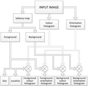
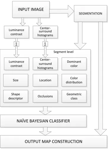
CHAPTER 2. SALIENCY 2.4. SEGMENT-BASED SALIENCY DETECTION
INPUT IMAGE
SEGMENTATION
Luminance contrast
Center-surround histograms
Luminance contrast
Center-surround histograms
Dominant color
Size Color
distribution Location
NAÏVE BAYESIAN CLASSIFIER
OUTPUT MAP CONSTRUCTION
∑Segment level ∑
Shape descriptor
Geometric class Occlusions
2.4. SEGMENT-BASED SALIENCY DETECTION CHAPTER 2. SALIENCY
This choice was due to publicly available source code and satisfactory
per-formance both from accuracy point of view and computational time. This
segmentation tool is based on mean-shift segmentation. To achieve better
object shape estimation the default parameters were tuned, their values
are reported in Table 2.1.
Table 2.1: Segmentation parameters
Minimum region area imheight×imwidth×0.005
Spatial bandwidth 10 Range bandwidth 7.5 Gradient window radius 2
Mixture parameter 0.3 Edge strength threshold 0.7
In this model saliency is detected mostly due to visual features that are
described below. Some of the features used cannot be extracted directly
from segment data. Their values are computed first on the whole image,
and segment-wise level is then obtained by averaging value of a feature on
pixels of that segment.
Colors have a great impact on the perception of objects. Gelasca et al.
in [24] described an experiment they conducted to discover colors impact
on saliency. Their study proved that some colors are more likely to attract
attention than overs. Figure 2.3 shows dependency of saliency likelihood
on the color of an object. In the original work the authors proposed to
convert image color values into CIELab colorspace. However, I have found
out that better color conversion is achieved with HSV colorspace. In the
original work, the authors assigned a weight to each color equal to the
fraction of attraction caused by this color during the experiments. Unlike
that, in this work prior value of saliency for each color is defined by its
position in the table of saliency likelihood, such that dark green has prior
CHAPTER 2. SALIENCY 2.4. SEGMENT-BASED SALIENCY DETECTION
Figure 2.3: Saliency dependency on colors
In addition, a feature taking into account colors distribution over an
image is included. This feature is based on observation that the
domi-nant color is very likely to belong to background and thus is unlikely to
be salient. For each segment its average color is computed and that match
with our colorspace. For each color tone a corresponding weight is
com-puted as follows:
wc0 = P 1
i∈Sc ai
,
wc =
wc0 −min(wi0)
max(w0i)−min(wi0), (2.1)
whereSc is a set of all segments assigned to colorc,ai is the area of segment
i,wc0 and wc are the unnormalized and normalized weights correspondingly.
As it was mentioned above human attention is sensitive to contrast.
In order to exploit this property luminance contrast is included into the
proposed model. This feature is measured on a downscaled by factor 8
version of an image. The motivation is that maximum contrast value is
usually observed on edges and glare spots, while downscaling allows to
catch global contrast changes. The luminance contrastLC is computed as
follows:
LC(x, y) = X
m
X
n
|L(x, y)−L(x+ m, y+ n)| √
m2 +n2 , (2.2)
2.4. SEGMENT-BASED SALIENCY DETECTION CHAPTER 2. SALIENCY
Figure 2.4: Luminance contrast feature output. From left to right: input image, luminance contrast without segmentation, luminance contrast after segmentation.
and m, n = {−2,−1,1,2} denote relative coordinates of neighbor pixels.
Example of luminance contrast output is shown in Figure 2.4.
The idea to measure the distance between foreground and background
for saliency detection was used in several previous works. The underlying
idea is that usually the histogram of the foreground object has a larger
extent than its surroundings. In our work we employ center-surround
histogram filter from [38] with slight modifications. The input image is
scanned by two rectangular windows Rf and Rs, both having a similar
area and Rs encloses Rf (thus Rf is a notch inside the window Rs). We
use the following size ratios of windows: [0.3, 0.7], which were defined
experimentally with respect to the minimum image dimension, as well as
the following three aspect ratios: [0.5 1 1.5]. Specifically the distance of
foreground and surrounding histograms is computed as follows:
dist(Rs, Rf) =
1 2
X(R
i f −R
i s)2 Rif + Ri
s
, (2.3)
where Ris, Rif are surrounding and foreground histograms, respectively. In
addition, unlike the original work, windows are moved with overlap of 0.1
with respect to the corresponding size of the window to eliminate boundary
effects within the scanning windows. Histogram distances are computed at
each scale and aspect ratio. Then, they are normalized and summed into a
CHAPTER 2. SALIENCY 2.4. SEGMENT-BASED SALIENCY DETECTION
Figure 2.5: Center-surround histogram filter. From left to right: input image, center-surround histogram output before segmentation, center-center-surround histogram output after segmentation.
average value of each global feature to each segment of the input image.
Figure 2.5 shows the principle of this feature.
In addition to visual feature, geometric features have been included.
The location feature has been included into the scheme due to the fact
that photographers generally place the object of interest to the center of
images. The location MS of the segment S is computed as follows:
MS = ((
X
x
X
y
f(x, y)p(x))2 + (X
x
X
y
f(x, y)q(y))2)12, (2.4)
with
f(x, y) = (
1 if x ∈ S and y ∈ S
0 otherwise, (2.5)
p(x) = mx
2 −x, (2.6)
q(y) = my
2 −y, (2.7)
and mx, my are the corresponding dimensions of the image. Considering size, the object of interest usually occupies a significant portion of the
im-age. Thus it is unlikely that a very small segment is salient. On the other
hand natural background like sky, ground, and forest usually occupy large
portion of area; thereby it is very unlikekly that a salient objects size
2.4. SEGMENT-BASED SALIENCY DETECTION CHAPTER 2. SALIENCY
relevant information about its saliency. Another feature exploiting
geomet-ric properties of a scene detects if a segment is occluded with others. The
intuition here is that normally, the main object of a scene is placed in front
of some background. Thus the background region becomes occluded by
the main object. There exist quite accurate methods for occlusion
detec-tion, however most of them require a lot of computation. Therefore, here I
propose a simple method of occlusion detection based on the segmentation
map. For computation of occlusion, firstly its necessary to compute spread
of each segment. Spread shows numerical extend of a segment relative to
its center of mass. One can think of spread as of a rectangle that is a
rough representation of an actual region occupied by a segment. Spread of
a segment is computed as follows:
mxs =
P
y∈Ys
k x ∈ [Xs<y> < cxs] k
kYs k
, (2.8)
pxs =
P
y∈Ys
k x ∈ [Xs<y> > cxs] k
kYs k
, (2.9)
mys =
P
x∈Xs
k y ∈ [Ys<x> < cys] k
k Xs k
, (2.10)
pys =
P
x∈Xs
ky ∈ [Ys<x> < cys] k
k Xs k
, (2.11)
where (cxs, cys) are coordinates of the center of mass of a segment s, Xs
and Ys are vectors holding all rows and colons of the segment s lies in,
(mxs, mys) and (pxs, pys) are coordinates of top left and bottom right
points of the rectangle representing the spread. Then, if two segments
have overlapping regions occlusion is detected by thresholding the area of
their intersection. Once occlusion is detected foreground and background
segments are detected by comparing their sizes. A segment with large
CHAPTER 2. SALIENCY 2.4. SEGMENT-BASED SALIENCY DETECTION
Figure 2.6: Occlusion feature output example. From left to right: input image, its seg-mentation map, occluded segments (drawn in black).
The background and foreground segments receive values of -1 and 1
re-spectfully. Thus for each segment there is an (n − 1)-element vector of
occlusions, where n is the number of all segments. Final value of this
fea-ture is calculated by taking mean value of this vector. Example output
of this feature is shown in Figure 2.4. In addition to occlusion, a feature
counting number of neighbour segments is included into the model. The
in-tuition here, is that normally an object of interest is composed from several
segments. These segments become neighbours to each other. On opposite
background objects are represented by a few segments. Thus counting the
number of neighbour segments adds some knowledge on the structure of
the scene.
Moreover, another feature responsive for geometric properties of a scene
is geometric class detector. It is based on the method described in [30].
This method performs geometric classification of surfaces found in 2-D
images. As an output the method provides such classes as sky, ground,
vertices. This classification is quite relevant for the task of saliency
predic-tion - rarely one would make a picture to capture ground, or sky, with some
obvious exceptions like a picture of a sunset or sunrise. Also experiments
have shown there is slight correlation between class vertices and
2.4. SEGMENT-BASED SALIENCY DETECTION CHAPTER 2. SALIENCY
Figure 2.7: Geometric class detector output. On the left the input image detector output is on the right. Different geometric classes are shaded with different colors. It is evident that vertices class (drawn in green) is related with the salient object of this image.
internal segmentation map. In the original work the authors used
super-pixel segmentation. Segmentation is quite expensive operation in terms of
time. Thereby, in order to avoid running two independent segmentation
operations, an interim segmentation map obtained while running initial
image segmentation is provided to the geometric classification method.
This interim segmentation map is oversegmented with respect to the final
segmentation map, thus to some extend its properties are close to that of
super-pixel segmentation. Since segments in interim and final
segmenta-tion maps are different matching is needed. Once geometric classes are
computed the 2-D map with pixel values equal to geometric class of
corre-sponding segments is constructed. This map is then used to compute the
geometric class of a segment in the final segmentation map by finding the
most frequent pixel value for the segment.
The shape of the object also can contribute to visual importance. For
instance, skewed objects are unlikely to be important parts of a scene.
An-other example is a rectangular objects that are likely to be a picture of
CHAPTER 2. SALIENCY 2.4. SEGMENT-BASED SALIENCY DETECTION
to describe the shape of an object, however, most of them require large
computational resource, or results in a high-order vector of data. For the
case of saliency detection there is no need to have very precise shape
infor-mation, on opposite only some properties of object’s shape are necessary.
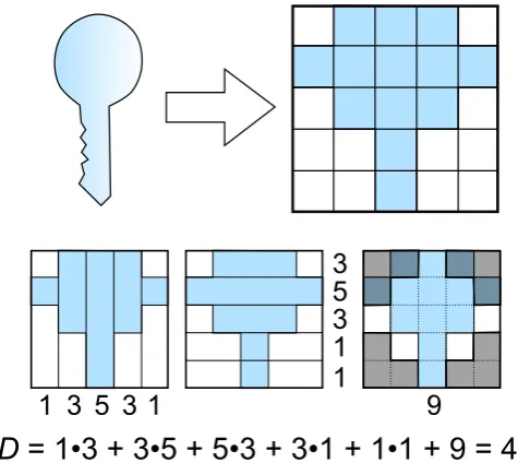
For this reason, here I propose a shape coding method that allows for very
compact description of shape properties. The visualization of feature
com-putation is shown in Figure 2.4. Each segment is fitted into 5x5 grid. If
a segment has line-like shape, then its shape is preserved and it occupies
only on row or column. The occupancy of grid cells is then used for three
descriptors: horizontal, vertical and center. Each of this descriptors counts
number of certain cells occupied by a segment according to the descriptor’s
map. The output of horizontal and vertical descriptors is then multiplied
element-by-element wise and summed up into one value that is later is
summed with the output of center descriptor. Once this feature computed
over the whole dataset the range of values of this feature is divided into six
regions. The index of this region is used as a final output of the feature.
Although this method seems to be naive the experiments have shown that
it is able to encode different types of shapes and moreover there is
corre-lation between output of this descriptor and ground-truth saliency data as
it is shown in Section 2.7.
Features described above represent each segment by a 12 element
vec-tor. For discrete features, namely for geometric context and occlusions
values are represented by multivariate indicator functions. Other features
are represented using gaussians. Modelling is done using probabilistic
framework. In this case it is Naive Bayesian classifier. Although some
of features used have correlation thus ruining the assumption of feature
independence, the performance of this classifier is satisfactory.
Classifica-tion is done per segment. Thus the output of the classifier holds saliency
corre-2.5. DEPTH-BASED SALIENCY DETECTION CHAPTER 2. SALIENCY
1 3 5 3 1 1 1 3 5 3
9
SD = 1•3 + 3•5 + 5•3 + 3•1 + 1•1 + 9 = 46
Figure 2.8: Shape descriptor
sponding saliency map using segmentation data. Learning was done using
expectation-maximization (EM) learning method. The overall scheme of
the method is shown in Figure 2.2. The evaluation results can be found in
Section 2.7.
2.5
Depth-based saliency detection
In this section a depth-based saliency detection method is presented. Here,
the main idea is that saliency to some extend can be estimated through
analysis of spacial layout of the scene. Unlike previous works in this topic,
depth information is not acquired using dedicated hardware, but instead is
estimated from input 2-D image. Recently, there have been achieved some
progress in the area of depth estimation that made this method possible.
One of the most important components in this method is depth
estima-tion that is done using the algorithm proposed by Saxena et al. in [50].
This method performs depth estimation modelling Markov Random Field
CHAPTER 2. SALIENCY 2.5. DEPTH-BASED SALIENCY DETECTION
Figure 2.9: Depth extraction [50]. Depth features are extracted at 3 scales. Relative and absolute feature vectors are composed from texton feature filter output.
into patches and a single depth value is then estimated for each patch. For
each patch two types of features are calculated: absolute and relative (see
Figure 2.9). Absolute feature estimates how far a patch is from the camera
plane, while the relative feature estimates whether two adjacent patches
are physically connected to each other in 3-D space. Both absolute and
rel-ative features are calculated using texture variations, texture gradients and
color. Original work applied depth estimation to outdoor scenes, mainly
including rural-like pictures. However, the test have shown that even on
other scenes depth estimation is quite reasonable. In my implementation
the grid of MRF is set to 50x50. Since it uses probababilistic framework
there is need to train its parameters. That has been done by learning
parameters on the database the original work was using. In addition, 50
indoor images acquired using stereo cameras were added into the database
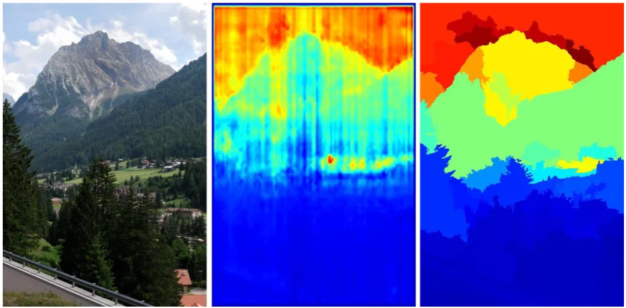
in order to improve performance for indoor scenes. Figure 2.10 shows an
example of depth estimation.
Similarly to the method described in Section 2.4 the detection is made
2.5. DEPTH-BASED SALIENCY DETECTION CHAPTER 2. SALIENCY
Figure 2.10: Depth estimation example. From left to right: input image, depth estimation map, depth estimation after segmentation. As one can notice after the segmentation procedure the estimation results in a quite realistic depth layout.
using Edison segmentation method [11]. Since the depth-estimation
im-plementation used works with MRF with the grid of 50x50 size, its output
is presented also as a grid. The depth of each segment then is defined as
the spatial average value of depth of the cells it is lying on.
Another common component with the visual-based method is
geometric-class detector [30]. However, here the motivation for its inclusion is
differ-ent. In the previous method this feature was responsible for layout
detec-tion, whereas here it adds some semantics to segments. Even though the
geometric-class detector provides classification over seven classes of surface
types, here these classes are merged into 3 final values: sky, ground and
others.
Although depth by itself provides some important information about
scene geometric properties, it is more of interest to exploit depth
relation-ship of different object in the scene. There are several features responsible
CHAPTER 2. SALIENCY 2.5. DEPTH-BASED SALIENCY DETECTION
farthest object in the scene. This feature returns distance to rear-plane.
Another feature describes sum of absolute difference of an object to its
adjacent objects divided by the number of neighbours. This feature is
re-sponsible for depth contrast, with intuition that if an object is distant from
its neighbours than probably it can be an object of interest. Likewise, if
two objects are close to each other it is likely they are both two parts of a
foreground or background scene. Figure 2.11 illustrates this principle.
Figure 2.11: Spatial closeness. Objects of the same context are placed spatially close to each other.
Analysing images of landscapes one can notice that they mostly consist
of flat surfaces. Such surfaces may have different orientation in z-y and z-x
axes with respect to the camera plane. For example consider shooting a
building in a city. It is obvious that the best view is achieved when the
elevation of the building is parallel to the camera plane. Thereby it is of
interest to measure the angle of an object with respect to the camera plane.
For this purpose a tangent-sensing feature is included. It is computed as
follows:
tany(r) =
1
kXr k
•X
Xr
(dx−dx−1) (2.12)
tany(obj) =
1
k Robj k
•X
Robj
(tany(r)) (2.13)
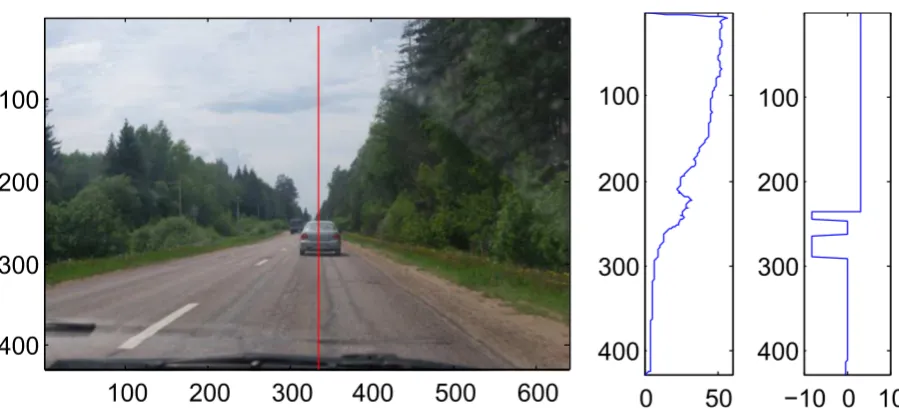
2.5. DEPTH-BASED SALIENCY DETECTION CHAPTER 2. SALIENCY
Figure 2.12: Tangent-like feature output example. From left to right: input image with the red line denoting the test column, estimated depth within the column, ZY-angle estimation per segment. It is clear visible how the rapid changes of angles in rows 200-300 corresponds to the body of the car. Although the tangent-like feature does not provide accurate angle estimation due to limitations of the depth estimation, still relative variance in plane orientation is detected.
is a set of all rows belonging to the object. As can be seen from (2.12)
tangent is computed in pixel-wise fashion. In the same way tangent in X
direction is computed by averaging column tangents.
To obtain more complete information about the scene the coordinates
of object’s geometric center of mass in X and Y axes are included into the
feature set. Here, the intuition is that normally a person would place an
object of interest close to the center of the frame rather on its boundary.
These features are computed in the same way as it was done in
segment-based method using Equations 2.6 and 2.7.
Portraits and group photos usually form a large portion of personal
albums. Our test have shown that depth estimation turns out to work
poor predicting z-coordinate for faces interfering with overall performance
CHAPTER 2. SALIENCY 2.5. DEPTH-BASED SALIENCY DETECTION
an image contains very flat objects, and depth estimation provides little
information. Thereby, to allow better performance two additional visual
features are employed. For each object its average color is measured and
matched to the closest representation from a fixed set of colors. This fixed
set consists of 9 tones, namely red, yellow, green, cyan, violet, pink, white,
grey and black. The colors are defined by splitting the HSV color space.
Color tones are obtained by dividing H component of HSV color space into
6 equal regions. Monotones are obtained by dividing V space into 3 equal
regions. Input color matched to grey tones if its S and V component satisfy
the following condition:
V < 0.1∨S < (0.1 + 0.01
V2 ) (2.14)
Another visual feature is color contrast computed based on object’s
domi-nant color difference with respect to all other objects as it is described in
2.4. To sum up the feature vector for each segment consists of ten
vari-ables. In addition, it is of interest to exploit pairwise labelling information
between adjacent objects. This is done through measuring similarity of
adjacent segments. Similarity is computed based on difference in depth.
The intuition behind this is that if two segments have close depth
estima-tion then it is likely that they are two parts of one object composed from
several segments and thus their saliency estimation should be the same.
Besides depth difference similarity is also defined by whether two segments
have the same dominant color and geometric class.
sim(i, j) =
(di −dj)2 +
9
P
k=1
(c[k]i−c[k]j)2, if gci = gcj
0, otherwise,
(2.15)
where di is the average depth of segment i, ci is its color histogram and
gci its geometric class. Here color histogram is obtained by counting the
2.5. DEPTH-BASED SALIENCY DETECTION CHAPTER 2. SALIENCY
INPUT IMAGE Depth estimation
Geometric classification Segmentation
Color contrast
Dominant color
Mean depth
Geometric class
Depth contrast
Distance to BG
tany
tanx (x,y)
CRF Saliency
CHAPTER 2. SALIENCY 2.6. SALIENCY EVALUATION DATASET
The modelling of saliency in this case is done using conditional random
field (CRM). Thus the optimization energy is described as follows:
E(sl,x,w) = X
i∈S
wsφsi(sli,x) +
X
(i,j)∈A
wpφpij(sli, slj,x) (2.16)
where the first term describes singleton energy and the later is pairwise
en-ergy; S is the set of all segments and A is the set of all adjacent segments.
The resulting graphical model is a loopy tree. Inference in this model is
done using graph-cut optimization for binary labelling [7]. Both singleton
and pairwise features are modelled using linear logistic regression.
Single-ton and pairwise parameters are jointly learnt using stochastic gradient
descent. The overall detection flow is shown in Figure 2.13.
2.6
Saliency evaluation dataset
Both for evaluation and training of the proposed models a ground-truth
database was created. Although there exists some datasets for
evalua-tion of saliency, there are not suitable for the proposed models. These
databases were collected using eye-trackers (for instance [34]1 and [58]2)
thereby ground truth data is represented by fixation points. However, the
methods proposed operate with segments rather than with separate pixels.
Thus there is need to perform matching of fixation points to segments.
Performing this task automatically is not possible due to limitations of
existing segmentation tools and sparse nature of fixation points. It is
com-mon with current segmentation tools that a real object is being represented
by several segments, and it often happens that fixation points can be
ab-sent in several object’s segments. In addition, tasks given to humans while
collecting these databases were different. For example, in [33] the authors


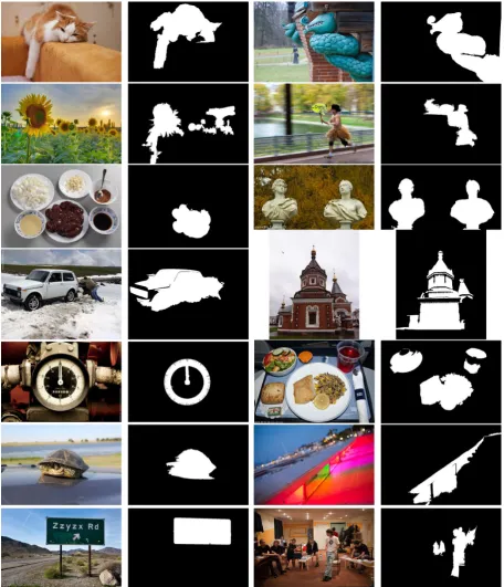

![Figure 2.20: Evaluation. A: original image, B: ground-truth map, C: depth-based method,D: segment-based method, E: Cheng et al [10], F: Liu et al [38], G: Judd et al [34], H:Achanta et al [3], I: Harel et al [29], J: Goferman et al [25], K: Margolin et al [43], L:Schauerte et al [51], M: Vikram et al [60], N: Ma et al [41], O: Hou et al [31], P: Seo et al[52], Q: Torralba et al [56], R: Fang et al [18]](https://thumb-us.123doks.com/thumbv2/123dok_us/563817.2055670/60.595.100.469.162.617/evaluation-original-segment-achanta-goferman-margolin-schauerte-torralba.webp)