Graph based Semi supervised Gene Mention Tagging

Graph-based Semi-supervised Gene Mention Tagging

Golnar Sheikhshab1,2_{, Elizabeth Starks}2_{, Aly Karsan}2_{, Anoop Sarkar}1_{, Inanc Birol}1,2

[email protected],{lstarks, akarsan}@bcgsc.ca,[email protected],[email protected]

1_{School of Computing Science, Simon Fraser University, Burnaby, BC, Canada}

2 _{Canada’s Michael Smith Genome Sciences Centre, British Columbia Cancer Agency, Vancouver, BC, Canada}

Abstract

The rapidly growing biomedical literature has been a challenging target for natu-ral language processing algorithms. One of the tasks these algorithms focus on is called named entity recognition (NER), often employed to tag gene mentions. Here we describe a new approach for this task, an approach that uses graph-based semi-supervised learning to train a Conditional Random Field (CRF) model. Benchmarking it on the BioCreative II Gene Mention tagging task, we achieved statistically significant improvements in F-measure over BANNER, a widely used biomedical NER system. We note that our tool is transductive and modular in nature, and can be integrated with other CRF-based supervised NER tools.

1 Introduction

Detecting biomedical named entities such as genes and proteins is one of the first steps in many natural language processing systems that analyze biomedical text. Finding relations between enti-ties, and expanding knowledge bases are examples of research that highly depend on the accuracy of gene and protein mention tagging.

Named entity recognition is typically modelled as a sequence tagging problem (Sha and Pereira, 2003). One of the most commonly used mod-els for sequence tagging is a Conditional Random Field (CRF) (Lafferty et al., 2001; Sha and Pereira, 2003).

Many popular and best performing biomedical named entity recognition systems, such as BAN-NER (Leaman et al., 2008), Gimli (Campos et al., 2013) and BANNER-CHEMDNER (Munkhdalai et al., 2015) use CRF as their core machine learn-ing model built on the MALLET toolkit (McCal-lum, 2002).

Inspired by the success of graph-based semi-supervised learning methods in other NLP tasks (Subramanya et al., 2010; Zhu et al., 2003; Subramanya and Bilmes, 2009; Alexandrescu and Kirchhoff, 2009; Liu et al., 2012; Saluja et al., 2014; Tamura et al., 2012; Talukdar et al., 2008; Das and Petrov, 2011), we integrated the graph based semi-supervised algorithm of Subramanya et al. (2010) and adapted their approach to im-prove on the results from BANNER. We show that our approach achieves a statistically signifi-cant improvement in terms of F-measure on the BioCreative II dataset for gene mention tagging.

Semi-supervised learning for gene mention tag-ging is not without precedent. There has been several semi-supervised approaches for the gene mention task and they have always been more successful than fully supervised approaches (Jiao et al., 2006; Ando, 2007; Campos et al., 2013; Munkhdalai et al., 2015).

Ando (2007) used a semi-supervised approach, Alternative Structure Optimization or ASO, in the BioCreative II gene mention shared task along with other extensions, such as using a lexicon or combining several classifiers. ASO ranked first among all competitors in the shared task compe-tition 2007. Ando reported usage of unlabeled data as the most useful part of his system improv-ing the F-measure of the baseline by 2.09 points where the complete (winning) system had a to-tal improvement of 3.23 points over the baseline CRF (Ando, 2007). Jiao et al. (2006) used condi-tional entropy over the unlabeled data combined with the conditional likelihood over the labeled data in the objective function of CRF (Jiao et al., 2006). Munkhdalai et al. (2015) trained word rep-resentations using Brown clustering (Brown et al., 1992) and word2vec (Mikolov et al., 2013) on MEDLINE and PMC document collections and used them as features along with traditional fea-tures in a CRF. Like many of these approaches we

also use unlabeled data to augment our baseline CRF model. In all these previous studies the un-labelled data was orders of magnitude more than labelled data and distinct from the test data.

In this paper we take a transductive approach and use the test set as our unlabelled data. More-over, our approach is orthogonal to all these ap-proaches and can be used to augment many of them. This approach can be easily implemented as a post-processing step in any system that uses a CRF model. Examples of such systems in-clude Gimli (Campos et al., 2013) and BANNER-CHEMNDNER (Munkhdalai et al., 2015). These tools have achieved the highest F-scores in the lit-erature after ASO (Ando, 2007). Our approach relies on the extraction of label distributions from the CRF and augments the decoding algorithm to incorporate the new information about gene men-tions from the graph-based learning approach we describe in this paper.

2 Method

Like many previous studies (Leaman et al., 2008; Munkhdalai et al., 2015; Campos et al., 2013), we formulate the gene mention tagging prob-lem as a word level sequence prediction probprob-lem, where labels for each word in the input are either Gene-Beginning, Gene-Inside, and Outside (not a gene). This representation is called IOB (for inside-outside-beginning). We applied a graph-based semi-supervised learning (SSL) approach, previously shown effective on a similar labelling task, part-of-speech tagging, for gene mention tag-ging. (Subramanya et al., 2010)

In graph-based SSL, a graph is constructed to represent partially labelled data. Each node in the graph represents a single word-level gene men-tion tagging decision and the edges between the nodes represent similarity between the nodes. The goal is to associate probability distributions over the IOB tags to all vertices. Label distributions for vertices that appear in labelled data are esti-mated based on the reference labels and propagate to vertices for unlabelled data in the graph. These label distributions are combined with the CRF de-coding algorithm used for labelling the test data. Graph-based SSL is categorized into inductive and transductive approaches. In inductive settings (e.g. Subramanya et al. (2010)), a model is trained and can be used as-is for unseen data. In transduc-tive settings however, the unlabelled data includes

test data. We took a transductive approach in con-structing our graph on the union of train set and test set as labelled and unlabelled data.

Since the graph is the cornerstone of the algo-rithm, let us describe its construction and usage before the overall algorithm.

2.1 Graph Construction

We use the following steps for constructing the graph for the gene mention tagging task adapted from the graph construction for part-of-speech tagging described in Subramanya et al. (2010):

1. Each vertex represents a 3-gram type and the middle word of this 3-gram is the word which is tagged as a gene mention using the IOB tags. The label distribution for this middle word is learned during graph propagation and subsequently combined with the CRF model at test time.

2. A vertex is represented by a vector of point-wise mutual information values between fea-ture instances and its 3-gram type.

3. Edge weights represent the similarity be-tween vertices and are obtained by comput-ing the cosine similarity of feature vectors of their two end vertices.

4. For each vertex only the K nearest neigh-bours are kept (default = 10).

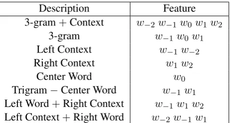
We considered several feature sets, namely con-textual features (Table 1), simplified concon-textual features (Table 2), all features from the base CRF model, and the most informative features from the base CRF model. We picked the simplified con-textual features based on preliminary results using cross-validation on our development set. To rep-resent a vertexvwith 3-gramw−1w0w1, we look at all occurrences of its 3-gram in the text, con-sider the larger contextw−2w−1w0w1w2 and get the lemmas of these words. v is represented by a vector of point-wise mutual information values be-tween all possible feature instances (e.g. all possi-ble lemmas forw−2) andw−1w0w1.

Description Feature 3-gram+Context w−2w−1w0w1w2

3-gram w−1w0w1

Left Context w−1w−2 Right Context w1w2

Center Word w0

Trigram−Center Word w−1w1 Left Word+Right Context w−1w1w2 Left Context+Right Word w−2w−1w1 Table 1: Complete set of contextual features.

Description Feature Left Context Word w−2

Left Word w−1 Center Word w0

Right Word w1 Right Context Word w2

Table 2: Simplified set of contextual features.

of the feature increases leaving extremely frequent features with relatively small weights.

2.2 Graph Propagation

In graph propagation we associate any given ver-texu with a label distributionXu that represents how likely we think each label is for that vertex.

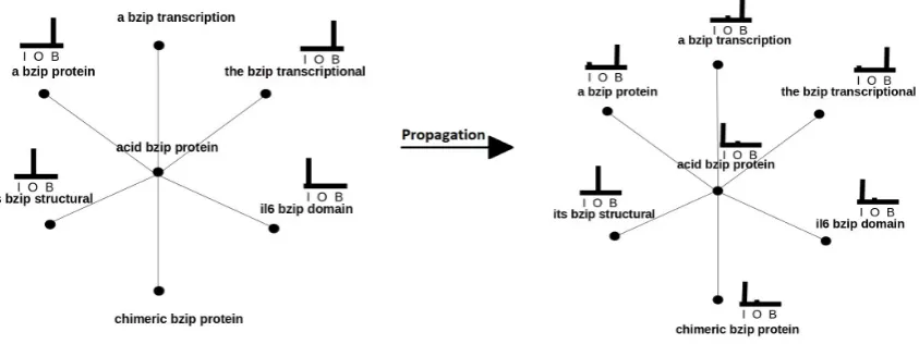
The goal of graph-based SSL is to propagate existing knowledge about the labels through the graph. The initial knowledge about graph nodes is provided by the labeled data and potentially some prior knowledge. Figure 1 shows how graph prop-agation can assign label distributions to unlabelled vertices and change the label distributions coming from labelled data.

Propagation is accomplished by optimizing an objective function over the label distributions at each node in the graph. The objective function consists of three types of constraints:

1. For any labeled vertexu, the associated label distributionXu should be close to the refer-ence distributionXˆu (obtained from labeled data);

2. Adjacent verticesuandkshould have similar label distributionsXuandXk;

3. The label distributions of all vertices should comply with the prior knowledge, if such knowledge exists, or be uniformly dis-tributed, otherwise.

The following objective function represents these three components:

C(X) = X u∈L

||Xu−Xˆu||22

+µX

u∈V

X

k∈N(u)

wu,k||Xu−Xk||22

+νX

u∈V

||Xu−U||22 (1)

where u and v are nodes in the graph, L is the set of labelled vertices,V is the set of all vertices,

N(u)is the set of neighbours ofu,U is the uni-form distribution over all labels, andµandν are weight constants for constraints 2 and 3, respec-tively. We used Euclidean distance as the distance metric.

While the first two terms in the objective func-tion, and their corresponding constraints make in-tuitive sense, the uniformity constraint needs fur-ther explanation. The rationale behind using dis-tance from uniform distribution is to avoid prefer-ring a label over others in the absence of strong evidence.

The objective function is optimized using stochastic gradient descent. We implement the op-timization algorithm for this as described in Sub-ramanya et al. (2010):

X_i(m)(y) =γi_k(y) i

γi(y) = ˆXi(y)δ(i∈L) + X

k∈N(i)

wi,kX_km−1(y) +ν_Y1

ki=δ(i∈L) +ν+µ

X

k∈N(i)

wi,k (2)

X_i(m)andX_i(m−1)denote the label distributions of vertexiin iterationsmandm−1, respectively,

δ(i ∈ L) is 1 if and only if iis a labeled vertex, andY is the number of labels.

2.3 Overall algorithm

On an input of a partially-labeled corpus, we first train a CRF model in a supervised fashion on the labeled data (crf-train, line 1); we then use this trained CRF model to assign label probability dis-tributions to each word in the entire (labeled + un-labeled) corpus (posterior decode, line 4). As a result, each n-gram token in the corpus has a la-bel distribution (the posteriors). For each n-gram typeu(a vertex in the graph), we find all instances (n-gram tokens) of u and average over the label distributions of these instances to get a label dis-tribution for u (token to type, line 5). Next, we perform graph-propagation (i.e. we optimize the objective function in equation 1) to learn the label distributions for all vertices. Finally, we linearly interpolate the trained CRF model and the label distributions from the graph:

Xint(t) =αXCRF(t) + (1−α)XGraph(t) (3) where t is a 3-gram token in a specific sen-tence,XCRF(t) denotes the posterior probability from the CRF model for the middle word in t,

XGraph(t)denotes the label distribution of the 3-gram type t after graph propagationn, and α ∈

[0,1] is the mixture parameter between the CRF and graph models. The best label for all words in the entire corpus is then found using Viterbi-decoding for the CRF usingXintinstead ofXCRF (viterbi-decode, line 7). Viterbi decoding provides us with the best label for every n-gram token in the unlabeled corpus, which implies that our labeled set has grown to include the unlabeled corpus. We re-train the CRF on this expanded training set (crf-train, line 8); and iterate until convergence.

Note that the steps indicated by lines 1, 4, and

Figure 2: Iterative semi-supervised training of CRF with label distributions from the graph. (Sub-ramanya et al., 2010).

8 work on the corpus whereas graph propagation in line 6 works on the graph. So, the step in line 5 takes us from corpus to the graph, and the step in line 7 takes us back from the graph to the corpus.

2.4 Integration with BANNER

BANNER (Leaman et al., 2008) is a well-known open-source biomedical named entity recognizer that is widely used. Many studies have used BANNER for gene mention tagging (Li et al., 2015; Hakala et al., 2015; Leaman et al., 2015; Pyysalo et al., 2015; Li et al., 2015; Lee et al., 2014; Leaman et al., 2013) and many have cited it as a biomedical NER system with good perfor-mance (Dai et al., 2015; Krallinger et al., 2015; Luo et al., 2016; Gonzalez et al., 2016; Hebbring et al., 2015).

BANNER uses CRF as its machine learning core, and we used it as our base CRF in lines 1 and 8 in Figure 2. We also modified BANNER’s source code in order to extract the posterior

Category Method Precision Recall F-Score

Baseline BANNER 86.27 85.57 84.90

Our methods _{Graph + postprocessing}Graph-based SSL 88.98_89.36 82.95_82.95 85.86_86.04

More recent methods BANNER-ChemDNER (2015)_{Gimli (2013)} 88.02_90.22 86.08_84.32 87.04_87.17

Best performing methods (Ando, 2007) 88.48 85.97 87.21 in BioCreative II challenge _{(Huang et al., 2007)}(Kuo et al., 2007) _84.9389.3 84.49_88.28 86.83_86.57

Table 3: Graph-based SSL improves BANNER by increasing the precision.

bilities from the underlying MALLET CRF model (line 4). These probabilities were used in lines 5 through 7 in Figure 2.

Furthermore, the lemmas we used as features in our graph construction (see section 2.1) came from BANNER’s lemmatizer.

BANNER also does some post-processing: it discards all the mentions that contain unmatched brackets. We ran our method with and without this post-processing step and verified its utility in our approach as well.

3 Experiments

We show improvements over BANNER on the dataset of BioCreative II Gene Mention Tagging Task. This data set contains 15,000 training sen-tences and 5,000 test sensen-tences. Annotations are given by the starting character index and finishing character index of the gene in the sentence (space characters are ignored). Some sentences have al-ternative annotations presented in a separate file.

The upper part of Table 3 shows the results of BANNER; Graph-Based SSL without processing; and Graph-Based SSL with post-processing. The hyper-parameters of Graph-Based SSL were chosen by cross-validation over different train/test splits with different hyper-parameters tested for each split (α = 0.02, µ = 10−6_{, ν = 10}−4_{, and number of iterations =} 2). Table 3 shows that the improvement we get in F-measure is due to better precision which is further boosted by dropping the candidates with unmatched parentheses (which is our only post-processing step).

The lower part of Table 3 puts our method in context. Although our method is competitive with these best performing methods in the literature, it has not outperformed any of them other than BANNER. Its precision however, is better than all other methods with the exception of Gimli. It would be interesting to integrate the graph-based approach to the ones with CRF as their machine

Type Of error Number Examples FN in both

BANNER and Graph 882 SST, R

FP in Graph 120 CD18, kinase, homeobox domain, transforming growth factor -_{beta, GRK6, POZ/Zn, HPR, E1B 19}

FP in BANNER 337 oxidase, dose Ara C, mouse amino acid sequence, Ann Arbor,K1F, wild-type R. sphaeroides 2.4.1, SAS GLM, 1.6-kb cDNA, SH2, E3 ubiquitin, Xp22.3

FN in BANNER 158 LDL, bZIP protein, SL1, NF-kappaB, Ig-like domain,immunoglobulin genes, signal transducer and activator of transcription 1, bcr, ACTH, GFR, wnt

FN in Graph 197 SH3A, EGF, VA1, CBP, Decidual/trophoblast prolactin-related_{protein, CA 50}

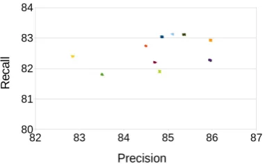
Figure 3: Precision and recall for different train/test splits and hyper-parameter choices. Each color represents a single train/test split. We in-clude only the Pareto optimal points for each split.

learning core (BANNER-ChemdNER, Gimli, and the approach of (Kuo et al., 2007)) to further test the utility of the graph approach.

3.1 Qualitative analysis

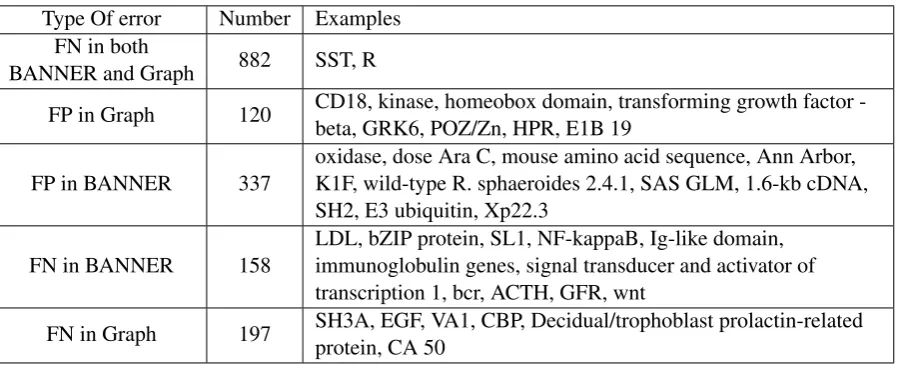
To understand the differences between BANNER and the graph propagation results, a human do-main expert compared the errors occurring in their respective outputs. Table 4 shows the number of these errors as well as some examples.

These examples illustrate two important obser-vations. First, there are examples of categories more general than genes in both false positives and false negatives for both systems. For example Ki-naseis a functional group of proteins;POZ/Zn, Ig-like domain, andSH2are protein domains; andE3 ubiquitinandNF-kappaBare gene families. Anec-dotal evidence suggests that this is due to presence of similar annotations in the training/test data set. For example the bZIP protein, a protein family, and Ig-like domain, a gene/protein functional do-main were both annotated as genes. This calls for a better gene mention corpus annotated according to more recent gene annotation guidelines. Sec-ond, there are some hard to explain false positives in BANNER. Examples includeAnn Arbor, a city in Michigan, SAS GLM, a type of statistical test, and1.6-kb cDNA, a molecular length. Our graph-based approach has eliminated these false posi-tives.

3.2 Cross validation study

We conducted extensive cross-validation experi-ments using different train and test splits in or-der to explore the hyper-parameter values and to

Figure 4: The same points as in Figure 3 shown as the difference from the Banner scores for the same train/test split. The origin in this graph is the BANNER score. Each cluster of points in Figure 3 becomes a line in this graph.

detect trends in the values that were optimal for this task. The results show that graph-propagation consistently improves results over BANNER.

Figures 3 and 4 were created by running graph-propagation over different train and test splits with different hyper-parameter values for each split. For each train/test split, we show only the Pareto optimal points (for each choice of hyper-parameters we include it in the graph only if the performance is not dominated by another choice in both recall and precision). Figure 3 illustrates two points: 1) the precision and recall for the differ-ent Pareto optimal points for each train/test split is very similar, and 2) overall the different train/test splits have similar precision and recall values. Fig-ure 4 shows the performance for each train/test split shown as the difference from the BANNER scores for that split. It shows that the precision scores of graph-propagation is always better than the BANNER baseline, while recall is sometimes worse. The F-scores for all train/test splits and for all Pareto optimal points in each split is always better than the BANNER baseline.

We can collect useful statistics about which hyper-parameter values are the most useful in graph-propagation in this task from the extensive set of experiments described above: for different train/test splits and for each split with different hyper-parameter values. Figure 5 shows the num-ber of times different hyper-parameter values have appeared in the set of Pareto optimal points over all the train/test splits.

distri-bution from the graph-propagation step. Higher

α values would prefer BANNER over graph-propagation. Figure 5 shows that smallerαvalues are preferred, which implies that the label distribu-tion produced through graph-propagadistribu-tion is found to be more useful than the label distribution pro-duced by BANNER. We also investigated the two extreme cases ofα= 0(only graph) andα = 1.0 (only BANNER followed by an extra Viterbi de-coding step), and observed that both of these op-tions were worse than the BANNER baseline.

In equation (1) higher ν values keep the label distribution at each vertex of the graph closer to the uniform distribution. Higher µ values would allow adjacent vertices to have a greater influence on the label distribution at the vertex. Figure 5 shows that, in our experiments, graph-propagation is sensitive to the values of µ. Lower µ values appear in Pareto optimal points more often. On the other hand, Figure 5 shows that graph-propagation is not as sensitive to different values ofνas long as it is not too high (10−1_{). This might be due to our} setting, where about 73% of vertices are labelled.

We looked for strong correlations between ν

values,µvalues, and number of iterations in graph propagation and found none.

Finally, for different iteration numbers of graph-propagation, we collected the frequency with which each number appeared in the Pareto opti-mal results. One iteration of graph-propagation produced 68 Pareto optimal points, two iterations produced 198 points, and three iterations pro-duced 120 points in our experiments. This shows that having more than one iteration of graph-propagation can improve the results.

Our algorithm (Figure 2) has two levels of itera-tions. One outer iteration (the while loop) and one

inner iteration in graph propagation. The numbers mentioned above refer to this inner iteration. All our results reported are for one outer iteration only. Our experiments in this paper were in a trans-ductive setting where the graph was constructed over the test and training data. For this reason we did not experiment extensively with more than one outer iteration. In future work, we plan to experiment with increasing the amount of unla-beled data, and in this setting explore increasing the number of outer iterations.

3.3 A note on scalability

The most time consuming step in our approach was graph construction, where the bootleneck is to compute the edge weights between any possi-ble vertex pairs. We experimented with a naive algorithm, where for every vertex pair the values of feature vectors for shared features were consid-ered, and the cosine similarity was computed. We also implemented a variation on it, where the sim-ilarities between all pairs sharing a specific feature instance were computed, and the contributions of individual feature instances were summed to give the final similarity between any given pair. The first algorithm was too slow as expected due to its

O(|V|2_{)time complexity; the second one was too} slow due to high frequency features. This is an important issue since the graph needs to be con-structed for our approach to work on a new dataset. Apart from the graph construction, the graph based approach is as scalable as CRF if a labeled train set is available for the new domain, as the CRF only needs to be trained on the new labelled set. If we wish to adapt the method in a domain where there is no labelled data in the target do-main, there is no need for any training.

0 50 100 150 200 1. E-06 1. E-05 1. E-04 1. E-03 1. E-02 1.

E-01 >1

Fr eq ue nc y µ 0 50 100 150 200 1. E-06 1. E-05 1. E-04 1. E-03 1. E-02 1.

E-01 >1

Fr eq ue nc y ν 0 20 40 60 80 100 120 0. 02 0. 04 0. 06 0.

08 _0.1

0. 12 0. 14 0. 16 0.

18 _0.2

0. 22 0. 24 0. 26 0.

28 _0.3

0. 32 >0 .3 2 Fr eq ue nc y α

Figure 5: These graphs show the number of times specific hyper-parameter valuesα,µandνappeared in Pareto optimal points over all train/test splits.

4 Conclusion and future directions Our results show that propagating labels from 3-grams present in training set to 3-3-grams only ap-pearing in the test set can significantly improve BANNER, a well-known frequently used biomed-ical named entity recognition system for the gene mention tagging task. Our cross-validation study shows the robustness of this improvement. We also presented qualitative comparison by a human domain expert. Our ideas for future work are cat-egorized into three groups:

1.Adding more unlabelled data: The only un-labelled data we included in the graph were the test data. Since the success of semi-supervised learn-ing methods is usually due to huge amount of un-labelled data, we plan to use many more PubMed abstracts to construct the graph. This however will be challenging because the graph construction can be time consuming as it was in our case due to high frequency features.

2. Constructing a better graph: Contextual features we used to construct our graph are only one of the feature sets that have been shown use-ful in gene mention tagging task. Other feature sets include orthographic features, contextual fea-tures learnt from neural networks, feafea-tures from parse trees. These features may also prove useful in constructing a graph that represents the simi-larity between gene mentions. Also, we can pre-process the raw sentences to collapse some collo-cations into one word so that the middle word in the 3-gram vertices are more meaningful.

3. Improving the latest approach: Although BANNER is one of the most frequently used biomedical named entity recognition system, it is not one with the best performance ever. Previous approaches have improved BANNER in a variety of ways, including semi-supervised learning. In particular, Munkhdalia et al. have achieved an F-measure of 87.04 by including word representa-tions learnt from massive unlabelled data as fea-tures (Munkhdalai et al., 2015) . We plan to test our approach on their freely available system.

5 Acknowledgements

The authors thank the funding organizations, Genome Canada, British Columbia Cancer Foun-dation, and Genome British Columbia for their partial support. The research was also partially

supported by the Natural Sciences and Engineer-ing Research Council of Canada (NSERC RGPIN 262313 and RGPAS 446348) to the fourth author.

References

Andrei Alexandrescu and Katrin Kirchhoff. 2009. Graph-based learning for statistical machine

trans-lation. InNAACL 2009.

Rie Kubota Ando. 2007. BioCreative II gene

men-tion tagging system at IBM Watson. In

Proceed-ings of the Second BioCreative Challenge Evalua-tion Workshop, volume 23, pages 101–103. Centro Nacional de Investigaciones Oncologicas (CNIO) Madrid, Spain.

Peter F Brown, Peter V Desouza, Robert L Mercer, Vincent J Della Pietra, and Jenifer C Lai. 1992. Class-based n-gram models of natural language. Computational linguistics, 18(4):467–479.

David Campos, S´ergio Matos, and Jos´e Lu´ıs Oliveira. 2013. Gimli: open source and high-performance

biomedical name recognition. BMC bioinformatics,

14(1):54.

Hong-Jie Dai, Po-Ting Lai, Yung-Chun Chang, and Richard Tzong-Han Tsai. 2015. Enhancing of chemical compound and drug name recognition us-ing representative tag scheme and fine-grained

tok-enization.Journal of cheminformatics, 7(S1):1–10.

Dipanjan Das and Slav Petrov. 2011. Unsupervised part-of-speech tagging with bilingual graph-based

projections. In Proceedings of the 49th Annual

Meeting of the Association for Computational Lin-guistics: Human Language Technologies-Volume 1, pages 600–609. Association for Computational Lin-guistics.

Graciela H Gonzalez, Tasnia Tahsin, Britton C Goodale, Anna C Greene, and Casey S Greene. 2016. Recent advances and emerging applications in text and data mining for biomedical discovery. Briefings in bioinformatics, 17(1):33–42.

Kai Hakala, Sofie Van Landeghem, Tapio Salakoski, Yves Van de Peer, and Filip Ginter. 2015. Appli-cation of the evex resource to event extraction and network construction: Shared task entry and result

analysis. BMC bioinformatics, 16(Suppl 16):S3.

Scott J Hebbring, Majid Rastegar-Mojarad, Zhan Ye, John Mayer, Crystal Jacobson, and Simon Lin. 2015. Application of clinical text data for

phenome-wide association studies (PheWASs).

Bioinformat-ics, 31(12):1981–1987.

Han-Shen Huang, Yu-Shi Lin, Kuan-Ting Lin, Cheng-Ju Kuo, Yu-Ming Chang, Bo-Hou Yang, I-Fang Chung, and Chun-Nan Hsu. 2007. High-recall gene mention recognition by unification of

second BioCreative challenge evaluation workshop, volume 23, pages 109–111. Centro Nacional de In-vestigaciones Oncologicas (CNIO) Madrid, Spain.

Feng Jiao, Shaojun Wang, Chi-Hoon Lee, Russell

Greiner, and Dale Schuurmans. 2006.

Semi-supervised conditional random fields for improved

sequence segmentation and labeling. In

Proceed-ings of the 21st International Conference on Com-putational Linguistics and the 44th annual meeting of the Association for Computational Linguistics, pages 209–216. Association for Computational Lin-guistics.

Martin Krallinger, Obdulia Rabal, Florian Leitner, Miguel Vazquez, David Salgado, Zhiyong Lu, Robert Leaman, Yanan Lu, Donghong Ji, Daniel M Lowe, et al. 2015. The chemdner corpus of

chemi-cals and drugs and its annotation principles. Journal

of cheminformatics, 7(S1):1–17.

Cheng-Ju Kuo, Yu-Ming Chang, Han-Shen Huang, Kuan-Ting Lin, Bo-Hou Yang, Yu-Shi Lin, Chun-Nan Hsu, and I-Fang Chung. 2007. Rich fea-ture set, unification of bidirectional parsing and dic-tionary filtering for high f-score gene mention

tag-ging. In Proceedings of the second BioCreative

challenge evaluation workshop, volume 23, pages 105–107. Centro Nacional de Investigaciones Onco-logicas (CNIO) Madrid, Spain.

John Lafferty, Andrew McCallum, and Fernando Pereira. 2001. Conditional random fields: Prob-abilistic models for segmenting and labeling

se-quence data. InICML.

Robert Leaman, Graciela Gonzalez, et al. 2008. Ban-ner: an executable survey of advances in biomedical

named entity recognition. InPacific Symposium on

Biocomputing, volume 13, pages 652–663. Citeseer.

Robert Leaman, Rezarta Islamaj Do˘gan, and Zhiy-ong Lu. 2013. Dnorm: disease name

normaliza-tion with pairwise learning to rank. Bioinformatics,

29(22):2909–2917.

Robert Leaman, Chih-Hsuan Wei, and Zhiyong Lu. 2015. tmchem: a high performance approach for chemical named entity recognition and

normaliza-tion. J. Cheminformatics, 7(S-1):S3.

Hee-Jin Lee, Tien Cuong Dang, Hyunju Lee, and Jong C Park. 2014. Oncosearch: cancer gene search

engine with literature evidence. Nucleic acids

re-search, page gku368.

Gang Li, Karen E Ross, Cecilia N Arighi, Yifan Peng, Cathy H Wu, and K Vijay-Shanker. 2015. mirtex: A text mining system for mirna-gene relation

extrac-tion. PLoS Comput Biol, 11(9):e1004391.

Shujie Liu, Chi-Ho Li, Mu Li, and Ming Zhou. 2012. Learning translation consensus with structured label

propagation. InACL 2012.

Yuan Luo, ¨Ozlem Uzuner, and Peter Szolovits. 2016. Bridging semantics and syntax with graph algorithmsstate-of-the-art of extracting biomedical

relations. Briefings in bioinformatics, page bbw001.

Andrew Kachites McCallum. 2002.

Mal-let: A machine learning for language toolkit. http://mallet.cs.umass.edu.

Tomas Mikolov, Kai Chen, Greg Corrado, and Jef-frey Dean. 2013. Efficient estimation of word

representations in vector space. arXiv preprint

arXiv:1301.3781.

Tsendsuren Munkhdalai, Meijing Li, Khuyagbaatar Batsuren, Hyeon Park, Nak Choi, and Keun Ho Ryu. 2015. Incorporating domain knowledge in chemical and biomedical named entity recognition with word

representations. J. Cheminformatics, 7(S-1):S9.

Sampo Pyysalo, Tomoko Ohta, Rafal Rak, Andrew Rowley, Hong-Woo Chun, Sung-Jae Jung, Sung-Pil Choi, Jun’ichi Tsujii, and Sophia Ananiadou. 2015. Overview of the cancer genetics and pathway

cura-tion tasks of bionlp shared task 2013. BMC

bioin-formatics, 16(Suppl 10):S2.

Avneesh Saluja, Hany Hassan, Kristina Toutanova, and Chris Quirk. 2014. Graph-based semi-supervised learning of translation models from monolingual

data. InACL 2014.

Fei Sha and Fernando Pereira. 2003. Shallow parsing

with conditional random fields. InNAACL.

Amarnag Subramanya and Jeff A Bilmes. 2009. En-tropic graph regularization in non-parametric

semi-supervised classification. InAdvances in Neural

In-formation Processing Systems, pages 1803–1811. Amarnag Subramanya, Slav Petrov, and Fernando

Pereira. 2010. Efficient graph-based

semi-supervised learning of structured tagging models. In Proceedings of the 2010 Conference on Empiri-cal Methods in Natural Language Processing, pages 167–176. Association for Computational Linguis-tics.

Partha Pratim Talukdar, Joseph Reisinger, Marius Pas¸ca, Deepak Ravichandran, Rahul Bhagat, and Fernando Pereira. 2008. Weakly-supervised acqui-sition of labeled class instances using graph random

walks. InEMNLP 2008.

Akihiro Tamura, Taro Watanabe, and Eiichiro Sumita. 2012. Bilingual lexicon extraction from comparable

corpora using label propagation. InEMNLP-CoNLL

2012.

Xiaojin Zhu, Zoubin Ghahramani, John Lafferty, et al.

2003. Semi-supervised learning using gaussian

fields and harmonic functions. InICML, volume 3,