Efficient Graph-Based Semi-Supervised Learning
of Structured Tagging Models
Amarnag Subramanya
Google Research Mountain View, CA 94043 [email protected]
Slav Petrov
Google Research New York, NY 10011 [email protected]
Fernando Pereira
Google Research Mountain View, CA 94043 [email protected]
Abstract
We describe a new scalable algorithm for semi-supervised training of conditional ran-dom fields (CRF) and its application to part-of-speech (POS) tagging. The algorithm uses a similarity graph to encourage similar n -grams to have similar POS tags. We demon-strate the efficacy of our approach on a do-main adaptation task, where we assume that we have access to large amounts of unlabeled data from the target domain, but no additional labeled data. The similarity graph is used dur-ing traindur-ing to smooth the state posteriors on the target domain. Standard inference can be used at test time. Our approach is able to scale to very large problems and yields significantly improved target domain accuracy.
1 Introduction
Semi-supervised learning (SSL) is the use of small amounts of labeled data with relatively large amounts of unlabeled data to train predictors. In some cases, the labeled data can be sufficient to pro-vide reasonable accuracy on in-domain data, but per-formance on even closely related out-of-domain data may lag far behind. Annotating training data for all sub-domains of a varied domain such as all of Web text is impractical, giving impetus to the develop-ment of SSL techniques that can learn from unla-beled data to perform well across domains. The ear-liest SSL algorithm is self-training (Scudder, 1965), where one makes use of a previously trained model to annotate unlabeled data which is then used to re-train the model. While self-training is widely
used and can yield good results in some applica-tions (Yarowsky, 1995), it has no theoretical guaran-tees except under certain stringent conditions, which rarely hold in practice(Haffari and Sarkar, 2007).
Other SSL methods include co-training (Blum and Mitchell, 1998), transductive support vector ma-chines (SVMs) (Joachims, 1999), and graph-based SSL (Zhu et al., 2003). Several surveys cover a broad range of methods (Seeger, 2000; Zhu, 2005; Chapelle et al., 2007; Blitzer and Zhu, 2008). A ma-jority of SSL algorithms are computationally expen-sive; for example, solving a transductive SVM ex-actly is intractable. Thus we have a conflict between wanting to use SSL with large unlabeled data sets for best accuracy, but being unable to do so because of computational complexity. Some researchers at-tempted to resolve this conflict by resorting to ap-proximations (Collobert et al., 2006), but those lead to suboptimal results (Chapelle et al., 2007).
Graph-based SSL algorithms (Zhu et al., 2003; Joachims, 2003; Corduneanu and Jaakkola, 2003; Belkin et al., 2005; Subramanya and Bilmes, 2009) are an important subclass of SSL techniques that have received much attention in the recent past, as they outperform other approaches and also scale eas-ily to large problems. Here one assumes that the data (both labeled and unlabeled) is represented by ver-tices in a graph. Graph edges link verver-tices that are likely to have the same label. Edge weights govern how strongly the labels of the nodes linked by the edge should agree.
Most previous work in SSL has focused on un-structured classification problems, that is, problems with a relatively small set of atomic labels. There
has been much less work on SSL for structured pre-diction where labels are composites of many atomic labels with constraints between them. While the number of atomic labels might be small, there will generally be exponentially many ways to combine them into the final structured label. Structured pre-diction problems over sequences appear for exam-ple in speech recognition, named-entity recogni-tion, and part-of-speech tagging; in machine trans-lation and syntactic parsing, the output may be tree-structured.
Altun et al. (2005) proposed a max-margin ob-jective for semi-supervised learning over structured spaces. Their objective is similar to that of manifold regularization (Belkin et al., 2005) and they make use of a graph as a smoothness regularizer. However their solution involves inverting a matrix whose size depends on problem size, making it impractical for very large problems. Brefeld and Scheffer (2006) present a modified version of the co-training algo-rithm for structured output spaces. In both of the above cases, the underlying model is based on struc-tured SVM, which does not scale well to very large datasets. More recently Wang et al. (2009) proposed to train a conditional random field (CRF) (Lafferty et al., 2001) using an entropy-based regularizer. Their approach is similar to the entropy minimization al-gorithm (Grandvalet and Bengio, 2005). The prob-lem here is that their objective is not convex and thus can pose issues for large problems. Further, graph-based SSL algorithms outperform algorithms graph-based on entropy minimization (Chapelle et al., 2007).
In this work, we propose a graph-based SSL method for CRFs that is computationally practical for very large problems, unlike the methods in the studies cited above. Our method is scalable be-cause it trains with efficient standard building blocks for CRF inference and learning and also standard graph label propagation machinery. Graph regular-izer computations are only used for training, so at test time, standard CRF inference can be used, un-like in graph-based transductive methods. Briefly, our approach starts by training a CRF on the source domain labeled data, and then uses it to decode unla-beled data from the target domain. The state posteri-ors on the target domain are then smoothed using the graph regularizer. Best state sequences for the unla-beled target data are then created by Viterbi
decod-ing with the smoothed state posteriors, and this au-tomatic target domain annotation is combined with the labeled source domain data to retrain the CRF.
We demonstrate our new method in domain adap-tation for a CRF part-of-speech (POS) tagger. While POS tagging accuracies have reached the level of inter-annotator agreement (>97%) on the standard PennTreebank test set (Toutanova et al., 2003; Shen et al., 2007), performance on out-of-domain data is often well below 90%, impairing language process-ing tasks that need syntactic information. For exam-ple, on the question domain used in this paper, the tagging accuracy of a supervised CRF is only 84%. Our domain adaptation algorithm improves perfor-mance to 87%, which is still far below in-domain performance, but a significant reduction in error.
2 Supervised CRF
We assume that we have a set of labeled source do-main examples Dl = {(xi,yi)}li=1, but only
un-labeled target domain examples Du = {xi}li+=ul+1.
Here xi = x(1)i x
(2)
i · · ·x
(|xi|)
i is the sequence of
words in sentence iandyi = yi(1)y
(2)
i · · ·y
(|xi|) i is
the corresponding POS tag sequence, withyi(j) ∈ Y
whereY is the set of POS tags. Our goal is to learn a CRF of the form:
p(yi|xi; Λ)∝exp Ni
X
j=1
K X
k=1
λkfk(y(j −1)
i ,y
(j)
i ,xi, j)
for the target domain. In the above equation, Λ = {λ1, . . . , λK} ∈RK,fk(y(j
−1)
i , y
(j)
i ,xi, j)is the
k-th feature function applied to two consecutive CRF states and some window of the input sequence, and λkis the weight of that feature. We discuss our
fea-tures in detail in Section 6. Given only labeled data
Dl, the optimal feature weights are given by:
Λ∗= argmin
Λ∈RK "
− l X
i=1
log p(yi|xi; Λ)+γkΛk2 #
(1)
Here kΛk2 is the squared `
2-norm and acts as the
regularizer, andγis a trade-off parameter whose set-ting we discuss in Section 6. In our case, we also have access to the unlabeled dataDufrom the target
graph over the unlabeled which will be used in our algorithm as a graph regularizer.
3 Graph Construction
Graph construction is the most important step in graph-based SSL. The standard approach for un-structured problems is to construct a graph whose vertices are labeled and unlabeled examples, and whose weighted edges encode the degree to which the examples they link should have the same la-bel (Zhu et al., 2003). Then the main graph con-struction choice is what similarity function to use for the weighted edges between examples. How-ever, in structured problems the situation is more complicated. Consider the case of sequence tag-ging we are studying. While we might be able to choose some appropriate sequence similarity to con-struct the graph, such as edit distance or a string kernel, it is not clear how to use whole sequence similarity to constrain whole tag sequences assigned to linked examples in the learning algorithm. Al-tun et al. (2005) had the nice insight of doing the graph construction not for complete structured ex-amples but instead for thepartsof structured exam-ples (also known as factors in graphical model ter-minology), which encode the local dependencies be-tween input data and output labels in the structured problem. However, their approach is too demanding computationally (see Section 5), so instead we use local sequence contexts as graph vertices, exploting the empirical observation that the part of speech of a word occurrence is mostly determined by its local context.
Specifically, the set V of graph vertices consists of all the word n-grams1 (types) that have occur-rences (tokens) in training sentences (labeled and unlabeled). We partitionV =Vl∪VuwhereVl
cor-responds to n-grams that occur at least once in the labeled data, andVucorresponds ton-grams that
oc-cur only in the unlabeled data.
Given a symmetric similarity function between types to be defined below, we link typesuandvwith
1
We pad then-grams at the beginning and end of sentences with appropriate dummy symbols.
Description Feature
Trigram + Context x1x2x3 x4x5
Trigram x2x3 x4
Left Context x1x2
Right Context x4x5
Center Word x2
Trigram – Center Word x2x4
Left Word + Right Context x2x4 x5
Left Context + Right Word x1x2 x4
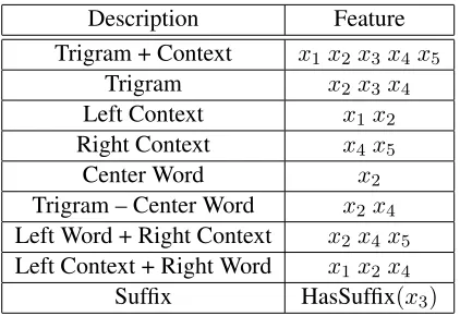
[image:3.612.322.533.53.198.2]Suffix HasSuffix(x3)
Table 1: Features we extract given a sequence of words “x1x2x3x4x5” where the trigram is “x2x3x4”.
an edge of weightwuv, defined as:
wuv = (
sim(u, v) ifv∈ K(u)oru∈ K(v)
0 otherwise
whereK(u)is the set ofk-nearest neighbors ofu ac-cording to the given similarity. For all experiments in this paper,n= 3andk= 5.
To define the similarity function, for each token of a given type in the labeled and unlabeled data, we extract a set of context features. For example, for the token x2 x3 x4 occurring in the sequence
x1 x2 x3 x4 x5, we use feature templates that
cap-ture the left (x1x2) and right contexts (x4x5).
Addi-tionally, we extract suffix features from the word in the middle. Table 1 gives an overview of the features that we used. For eachn-gram type, we compute the vector of pointwise mutual information (PMI) val-ues between the type and each of the features that occur with tokens of that type. Finally, we use the cosine distance between those PMI vectors as our similarity function.
[the conference on]
[whose book on] [the auction on] [U.N.-backed conference on]
[the conference speakers] [to schedule a]
[image:4.612.120.496.55.209.2][to postpone a] VB
[to ace a]
[to book a] [to run a]
[to start a] NN NN
NN VB
VB
[you book a]
[you rent a] [you log a]
[you unrar a] [to book some]
[to approve some] VB
[to fly some]
[to approve parental-consent]
6
4 3
[the book that]
[the job that]
[the constituition that] [the movie that]
[the city that]
NN NN [a movie agent]
[a clearing agent] [a book agent]
7
4
6
Figure 1: Vertices with center word ‘book’ and their local neighborhoods, as well as the shortest-path distance between them. Note that the noun (NN) and verb (VB) interpretations form two disjoint connected components.
It is remarkable that the neighborhoods are co-herent, showing very similar syntactic configura-tions. Furthermore, different vertices that (should) have the same label are close to each other, form-ing connected components for each part-of-speech category (for nouns and verbs in the figure). We ex-pect the similarity graph to provide information that cannot be expressed directly in a sequence model. In particular, it is not possible in a CRF to directly enforce the constraint that similar trigrams appear-ing in different sentences should have similar POS tags. This constraint however is important dur-ing (semi-supervised) learndur-ing, and is what makes our approach different and more effective than self-training.
In practice, we expect two main benefits from our graph-based approach. First, the graph allows new features to be discovered. Many words occur only in the unlabeled data and a purely supervised CRF would not be able to learn feature weights for those observations. We could use self-training to learn weights for those features, but self-training just tends to reinforce the knowledge that the supervised model already has. The similarity graph on the other hand can link events that occur only in the unlabeled data to similar events in the labeled data. Further-more, because the graph is built over types rather than tokens, it will encourage the same interpreta-tion to be chosen for similar trigrams occurring in different sentences. For example, the word ‘unrar’ will most likely not occur in the labeled training data. Seeing it in the neighborhood of words for
which we know the POS tag will help us learn the correct POS tag for this otherwise unknown word (see Figure 1).
Second, the graph propagates adjustments to the weights of known features. Many words occur only a handful of times in our labeled data, resulting in poor estimates of their contributions. Even for fre-quently occurring events, their distribution in the tar-get domain might be different from their distribution in the source domain. While self-training might be able to help adapt to such domain changes, its ef-fectiveness will be limited because the model will always be inherently biased towards the source do-main. In contrast, labeled vertices in the similar-ity graph can help disambiguate ambiguous contexts and correct (some of) the errors of the supervised model.
4 Semi-Supervised CRF
Given unlabeled data Du, we only have access to
the prior p(x). As the CRF is a discriminative model, the lack of label information renders the CRF weights independent ofp(x)and thus we can-not directly utilize the unlabeled data when train-ing the CRF. Therefore, semi-supervised approaches to training discriminative models typically use the unlabeled data to construct a regularizer that is used to guide the learning process (Joachims, 1999; Lawrence and Jordan, 2005). Here we use the graph as a smoothness regularizer to train CRFs in a semi-supervised manner.
Algorithm 1Semi-Supervised CRF Training
Λs=crf-train(Dl,Λ0) SetΛ(0t)= Λ(s)
whilenot convergeddo
{p}=posterior decode(Du,Λold) {q}=token to type({p})
{ˆq}=graph propagate({q})
Du(1)=viterbi decode({ˆq},Λold) Λ(nt+1) =crf-train(Dl∪ D(1)u ,Λ(nt))
end while Return lastΛ(t)
simple (and convex) steps: Given a set of CRF pa-rameters, we first compute marginals over the un-labeled data (posterior decode). The marginals over tokens are then aggregated to marginals over types (token to type), which are used to initial-ize the graph label distributions. After running la-bel propagation (graph propagate), the posteriors from the graph are used to smooth the state posteri-ors. Decoding the unlabeled data (viterbi decode) produces a new set of automatic annotations that can be combined with the labeled data to retrain the CRF using the supervised CRF training objective (crf-train). These steps, summarized in Algorithm 1, are iterated until convergence.
4.1 Posterior Decoding
LetΛ(nt)(trefers to target domain) represent the
esti-mate of the CRF parameters for the target domain af-ter then-th iteration.2In this step, we use the current parameter estimates to compute the marginal proba-bilities
p(yi(j)|xi; Λn(t)) 1≤j ≤ |xi|, i∈ Dl
over POS tags for every word positionjfori index-ing over sentences inDl∪ Du.
4.2 Token-to-Type Mapping
Recall that our graph is defined over types while the posteriors computed above involve particular to-kens. We accumulate token-based marginals to cre-ate type marginals as follows. For a sentenceiand word position j in that sentence, letT(i, j) be the
2In the first iteration, we initialize the target domain
param-eters to the source domain paramparam-eters:Λ(t)0 = Λ(s).
trigram (graph node) centered at positionj. Con-versely, for a trigram typeu, let T−1(u) be the set of actual occurrences (tokens) of that trigramu; that is, all pairs(i, j)whereiis the index of a sentence where u occurs and j is the position of the center word of an occurrence ofuin that sentence. We cal-culate type-level posteriors as follows:
qu(y), 1 |T−1(u)|
X
(i,j)∈T−1(u)
p(yi(j)|xi; Λ(nt)) .
This combination rule connects the token-centered CRF with the type-centered graph. Other ways of combining the token marginals, such as using weights derived from the entropies of marginals, might be worth investigating.
4.3 Graph Propagation
We now use our similarity graph (Section 3) to smooth the type-level marginals by minimizing the following convex objective:
C(q) = X u∈Vl
kru−quk2
+µ X
u∈V,v∈N(i)
wuvkqu−qvk2+ν X
u∈V
kqu−Uk2
s.t. X
y
qu(y) = 1∀u& qu(y)≥0∀u, y (2)
where q = {q1,q2, . . .q|V|}. The setting of the
hyperparametersµandν will be discussed in Sec-tion 6,N(u)is the set of neighbors of node u, and
ruis the empirical marginal label distribution for
tri-gramuin the labeled data. We use a squared loss to penalize neighboring nodes that have different label distributions: kqu −qvk2 = Py(qu(y)−qv(y))2,
additionally regularizing the label distributions to-wards the uniform distribution U over all possible labelsY. It can be shown that the above objective is convex inq.
Our graph propagation objective can be seen as a multi-class generalization of the quadratic cost crite-rion (Bengio et al., 2007). The first term in the above objective requires that we respect the information in our labeled data. The second term is the graph smoothness regularizer which requires that theqi’s
squared-error sense. This implies that verticesuand vare likely to have similar marginals over POS tags. The last term is a regularizer and encourages all type marginals to be uniform to the extent that is allowed by the first two terms. If a unlabeled vertex does not have a path to any labeled vertex, this term en-sures that the converged marginal for this vertex will be uniform over all tags, ensuring that our algorithm performs at least as well as a standard self-training based algorithm, as we will see later.
While the objective in Equation 2 admits a closed form solution, it involves inverting a matrix of or-der|V|and thus we use instead the simple iterative update given by
q(um)(y) = γu(y)
κu
where
γu(y) =ru(y)δ(u∈Vl)
+ X
v∈N(u)
wuvqv(m−1)(y) +νU(y),
κu =δ(u∈Vl) +ν+µ X
v∈N(u)
wuv (3)
where m is the iteration index andδ is the indica-tor function that returns 1 if and only if the con-dition is true. The iterative procedure starts with
q(0)u (y) = qu(y) as given in the previous section.
In all our experiments we run 10 iterations of the above algorithm, and we denote the type marginals at completion byq∗u(y).
4.4 Viterbi Decoding
Given the type marginals computed in the previous step, we interpolate them with the original CRF to-ken marginals. This interpolation between type and token marginals encourages similarn-grams to have similar posteriors, while still allowing n-grams in different sentences to differ in their posteriors. For each unlabeled sentenceiand word positionj in it, we calculate the following interpolated tag marginal:
ˆ
p(y(ij)=y|xi) =αp(yi(j)=y|xi; Λ(nt)) + (1−α)q∗T(m,n)(y) (4)
where α is a mixing coefficient which reflects the relative confidence between the original posteriors from the CRF and the smoothed posteriors from the graph. We discuss how we setαin Section 6.
The interpolated marginals summarize all the in-formation obtained so far about the tag distribution at each position. However, if we were to use them on their own to select the most likely POS tag sequence, the first-order tag dependencies modeled by the CRF would be mostly ignored. This happens because the type marginals obtained from the graph after label propagation will have lost most of the sequence in-formation. To enforce the first-order tag dependen-cies we therefore use Viterbi decoding over the com-bined interpolated marginals and the CRF transition potentials to compute the best POS tag sequence for each unlabeled sentence. We refer to these 1-best transcripts asy∗i, i∈ Du.
4.5 Re-training the CRF
Now that we have successfully labeled the unlabeled target domain data, we can use it in conjunction with the source domain labeled data to re-train the CRF:
Λ(nt+1) =argmin
Λ∈RK
− l X
i=1
log p(yi|xi; Λ(nt))
−η
l+u X
i=l+1
log p(yi∗|xi; Λn(t))+γkΛk2
(5)
whereη andγ are hyper-parameters whose setting we discuss in Section 6. Given the new CRF pa-rametersΛwe loop back to step 1 (Section 4.1) and iterate until convergence. It is important to note that every step of our algorithm is convex, although their combination clearly is not.
5 Related Work
We mentioned already the algorithm of Altun et al. (2005), which is unlikely to scale up because its dual formulation requires the inversion of a ma-trix whose size depends on the graph size. Gupta et al. (2009) also constrain similar trigrams to have similar POS tags by forming cliques of similar tri-grams and maximizing the agreement score over these cliques. Computing clique agreement poten-tials however is NP-hard and so they propose ap-proximation algorithms that are still quite complex computationally. We achieve similar effects by us-ing our simple, scalable convex graph regularization framework. Further, unlike other graph-propagation algorithms (Alexandrescu and Kirchhoff, 2009), our approach is inductive. While one might be able to make inductive extensions of transductive ap-proaches (Sindhwani et al., 2005), these usually re-quire extensive computational resources at test time.
6 Experiments and Results
We use the Wall Street Journal (WSJ) section of the Penn Treebank as our labeled source domain training set. We follow standard setup procedures for this task and train on sections 00-18, compris-ing of 38,219 POS-tagged sentences with a total of 912,344 words. To evaluate our domain-adaptation approach, we consider two different target domains: questions and biomedical data. Both target do-mains are relatively far from the source domain (newswire), making this a very challenging task.
The QuestionBank (Judge et al., 2006), provides an excellent corpus consisting of 4,000 questions that were manually annotated with POS tags and parse trees. We used the first half as our develop-ment set and the second half as our test set. Ques-tions are difficult to tag with WSJ-trained taggers primarily because the word order is very different than that of the mostly declarative sentences in the training data. Additionally, the unknown word rate is more than twice as high as on the in-domain de-velopment set (7.29% vs. 3.39%). As our unla-beled data, we use a set of 10 million questions collected from anonymized Internet search queries. These queries were selected to be similar in style and length to the questions in the QuestionBank.3
3
In particular, we selected queries that start with an English function word that can be used to start a question (what, who,
As running the CRF over 10 million sentences can be rather cumbersome and probably unnecessary, we randomly select 100,000 of these queries and treat this asDu. Because the graph nodes and the features
used in the similarity function are based onn-grams, data sparsity can be a serious problem, and we there-fore use the entire unlabeled data set for graph con-struction. We estimate the mutual information-based features for each trigram type over all the 10 million questions, and then construct the graph over only the set of trigram types that actually occurs in the 100,000 random subset and the WSJ training set.
For our second target domain, we use the Penn BioTreebank (PennBioIE, 2005). This corpus con-sists of 1,061 sentences that have been manually an-notated with POS tags. We used the first 500 sen-tences as a development set and the remaining 561 sentences as our final test set. The high unknown word rate (23.27%) makes this corpus very difficult to tag. Furthermore, the POS tag set for this data is a super-set of the Penn Treebank’s, including the two new tags HYPH (for hyphens) and AFX (for com-mon post-modifiers of biomedical entities such as genes). These tags were introduced due to the im-portance of hyphenated entities in biomedical text, and are used for 1.8% of the words in the test set. Any tagger trained only on WSJ text will automati-cally predict wrong tags for those words. For unla-beled data we used 100,000 sentences that were cho-sen by searching MEDLINE for abstracts pertaining to cancer, in particular genomic variations and muta-tions (Blitzer et al., 2006). Since we did not have ac-cess to additional unlabeled data, we used the same set of sentences as target domain unlabeled data,Du.
The graph here was constructed over the 100,000 un-labeled sentences and the WSJ training set. Finally, we remind the reader that we did not use label infor-mation for graph construction in either corpus.
6.1 Baselines
Our baseline supervised CRF is competitive with state-of-the-art discriminative POS taggers (Toutanova et al., 2003; Shen et al., 2007), achieving 97.17% on the WSJ development set (sections 19-21). We use a fairly standard set of features, includ-ing word identity, suffixes and prefixes and detectors
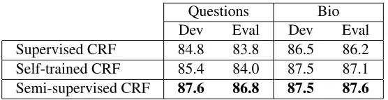
Questions Bio
Dev Eval Dev Eval
Supervised CRF 84.8 83.8 86.5 86.2
Self-trained CRF 85.4 84.0 87.5 87.1
[image:8.612.168.446.53.125.2]Semi-supervised CRF 87.6 86.8 87.5 87.6
Table 2: Domain adaptation experiments. POS tagging accuracies in %.
for special characters such as dashes and digits. We do not use of observation-dependent transition fea-tures. Both supervised and semi-supervised models are regularized with a squared `2-norm regularizer
with weight set to0.01.
In addition to the supervised baseline trained ex-clusively on the WSJ, we also consider a semi-supervised self-trained baseline (“Self-trained CRF” in Table 2). In this approach, we first train a su-pervised CRF on the labeled data and then do semi-supervised training without label propagation. This is different from plain self-training because it aggre-gates the posteriors over tokens into posteriors over types. This aggregation step allows instances of the same trigram in different sentences to share infor-mation and works better in practice than direct self-training on the output of the supervised CRF.
6.2 Domain Adaptation Results
The data set obtained concatenating the WSJ train-ing set with the 10 million questions had about 20 million trigram types. Of those, only about 1.1 mil-lion trigram types occurred in the WSJ training set or in the 100,000 sentence sub-sample. For the biomedical domain, the graph had about 2.2 mil-lion trigrams. For all our experiments we set hy-perparameters as follows: for graph propagation, µ = 0.5, ν = 0.01, for Viterbi decoding mixing, α= 0.6, for CRF re-training,η= 0.001, γ= 0.01. These parameters were chosen based on develment set performance. All CRF objectives were op-timized using L-BFGS (Bertsekas, 2004).
Table 2 shows the results for both domains. For the question corpus, the supervised CRF performs at only 85% on the development set. While it is al-most impossible to improve in-domain tagging ac-curacy and tagging is therefore considered a solved problem by many, these results clearly show that the problem is far from solved. Self-training im-proves over the baseline by about 0.6% on the
de-velopment set. However the gains from self-training are more modest (0.2%) on the evaluation (test) set. Our approach is able to provide a more solid im-provement of about 3% absolute over the super-vised baseline and about 2% absolute over the self-trained system on the question development set. Un-like self-training, on the question evaluation set, our approach provides about 3% absolute improvement over the supervised baseline. For the biomedical data, while the performances of our approach and self-training are statistically indistinguishable on the development set, we see modest gains of about 0.5% absolute on the evaluation set. On the same data, we see that our approach provides about 1.4% absolute improvement over the supervised baseline.
7 Analysis & Conclusion
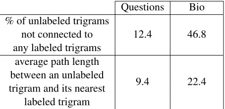
The results suggest that our proposed approach pro-vides higher gains relative to self-training on the question data than on the biomedical corpus. We hypothesize that this caused by sparsity in the graph generated from the biomedical dataset. For the ques-tions graph, the PMI statistics were estimated over 10 million sentences while in the case of the biomed-ical dataset, the same statistics were computed over just 100,000 sentences. We hypothesize that the lack of well-estimated features in the case of the biomed-ical dataset leads to a sparse graph.
Questions Bio % of unlabeled trigrams
12.4 46.8
not connected to any labeled trigrams
average path length
9.4 22.4
between an unlabeled trigram and its nearest
[image:9.612.73.300.54.164.2]labeled trigram
Table 3: Analysis of the graphs constructed for the two datasets discussed in Section 6. Unlabeled trigrams occur in the target domain only. Labeled trigrams occur at least once in the WSJ training data.
the other hand, for the question corpus, only about 12% of the target domain trigrams are disconnected, and the average path length is about 9. These re-sults clearly show the sparse nature of the biomed-ical graph. We believe that it is this sparsity that causes the graph propagation tonothave a more no-ticeable effect on the final performance. It is note-worthy that making use of even such a sparse graph does not lead to any degradation in results, which we attribute to the choice of graph-propagation regular-izer (Section 4.3).
We presented a simple, scalable algorithm for training structured prediction models in a semi-supervised manner. The approach is based on using as a regularizer a nearest-neighbor graph constructed over trigram types. Our results show that the ap-proach not only scales to large datasets but also pro-duces significantly improved tagging accuracies.
References
A. Alexandrescu and K. Kirchhoff. 2009. Graph-based learning for statistical machine translation. InNAACL. Y. Altun, D. McAllester, and M. Belkin. 2005. Max-imum margin semi-supervised learning for structured variables. InAdvances in Neural Information Process-ing Systems 18, page 18.
M. Belkin, P. Niyogi, and V. Sindhwani. 2005. On man-ifold regularization. InProc. of the Conference on Ar-tificial Intelligence and Statistics (AISTATS).
Y. Bengio, O. Delalleau, and N. L. Roux, 2007. Semi-Supervised Learning, chapter Label Propogation and Quadratic Criterion. MIT Press.
D Bertsekas. 2004. Nonlinear Programming. Athena Scientific Publishing.
J. Blitzer and J. Zhu. 2008. ACL 2008 tutorial on Semi-Supervised learning.
J. Blitzer, R. McDonald, and F. Pereira. 2006. Domain adaptation with structural correspondence learning. In
EMNLP ’06.
A. Blum and T. Mitchell. 1998. Combining labeled and unlabeled data with co-training. InCOLT: Proceed-ings of the Workshop on Computational Learning The-ory.
U. Brefeld and T. Scheffer. 2006. Semi-supervised learn-ing for structured output variables. InICML06, 23rd International Conference on Machine Learning. O. Chapelle, B. Scholkopf, and A. Zien. 2007.
Semi-Supervised Learning. MIT Press.
R. Collobert, F. Sinz, J. Weston, L. Bottou, and T. Joachims. 2006. Large scale transductive svms.
Journal of Machine Learning Research.
A. Corduneanu and T. Jaakkola. 2003. On informa-tion regularizainforma-tion. InUncertainty in Artificial Intelli-gence.
Y. Grandvalet and Y. Bengio. 2005. Semi-supervised learning by entropy minimization. InCAP.
R. Gupta, S. Sarawagi, and A. A. Diwan. 2009. General-ized collective inference with symmetric clique poten-tials.CoRR, abs/0907.0589.
G. R. Haffari and A. Sarkar. 2007. Analysis of semi-supervised learning with the Yarowsky algorithm. In
UAI.
F. Huang and A. Yates. 2009. Distributional represen-tations for handling sparsity in supervised sequence-labeling. In ACL-IJCNLP ’09: Proceedings of the Joint Conference of the 47th Annual Meeting of the ACL and the 4th International Joint Conference on Natural Language Processing of the AFNLP: Volume 1. Association for Computational Linguistics. H. Daume III. 2007. Frustratingly easy domain
adapta-tion. InProceedings of the 45th Annual Meeting of the Association of Computational Linguistics, pages 256–263, Prague, Czech Republic, June. Association for Computational Linguistics.
T. Joachims. 1999. Transductive inference for text clas-sification using support vector machines. InProc. of the International Conference on Machine Learning (ICML).
Thorsten Joachims. 2003. Transductive learning via spectral graph partitioning. In Proc. of the Interna-tional Conference on Machine Learning (ICML). J. Judge, A. Cahill, and J. van Genabith. 2006.
J. Lafferty, A. McCallum, and F. Pereira. 2001. Con-ditional random fields: Probabilistic models for seg-menting and labeling sequence data. InProc. of the In-ternational Conference on Machine Learning (ICML). N. D. Lawrence and M. I. Jordan. 2005. Semi-supervised
learning via gaussian processes. InNIPS.
PennBioIE. 2005. Mining the bibliome project. In
http://bioie.ldc.upenn.edu/.
H. J. Scudder. 1965. Probability of Error of some Adap-tive Pattern-Recognition Machines. IEEE Transac-tions on Information Theory, 11.
M. Seeger. 2000. Learning with labeled and unlabeled data. Technical report, University of Edinburgh, U.K. L. Shen, G. Satta, and A. Joshi. 2007. Guided learning
for bidirectional sequence classification. InACL ’07. V. Sindhwani, P. Niyogi, and M. Belkin. 2005. Beyond
the point cloud: from transductive to semi-supervised learning. InProc. of the International Conference on Machine Learning (ICML).
A. Subramanya and J. A. Bilmes. 2009. Entropic graph regularization in non-parametric semi-supervised
clas-sification. In Neural Information Processing Society (NIPS), Vancouver, Canada, December.
K. Toutanova, D. Klein, C. D. Manning, and Y. Singer. 2003. Feature-rich part-of-speech tagging with a cyclic dependency network. InHLT-NAACL ’03. Y. Wang, G. Haffari, S. Wang, and G. Mori. 2009.
A rate distortion approach for semi-supervised condi-tional random fields.
D. Yarowsky. 1995. Unsupervised word sense disam-biguation rivaling supervised methods. In Proceed-ings of the 33rd Annual Meeting of the Association for Computational Linguistics.
X. Zhu, Z. Ghahramani, and J. Lafferty. 2003. Semi-supervised learning using gaussian fields and har-monic functions. InProc. of the International Con-ference on Machine Learning (ICML).