R E S E A R C H
Open Access
Quantization in zero leakage helper data
schemes
Joep de Groot
1,4, Boris Škori´c
2, Niels de Vreede
3and Jean-Paul Linnartz
1*Abstract
A helper data scheme (HDS) is a cryptographic primitive that extracts a high-entropy noise-free string from noisy data. Helper data schemes are used for preserving privacy in biometric databases and for physical unclonable functions. HDSs are known for the guided quantization of continuous-valued sources as well as for repairing errors in discrete-valued (digitized) sources. We refine the theory of helper data schemes with the zero leakage (ZL) property, i.e., the mutual information between the helper data and the extracted secret is zero. We focus on quantization and prove that ZL necessitates particular properties of the helper data generating function: (1) the existence of “sibling points”, enrollment values that lead to the same helper data but different secrets and (2) quantile helper data. We present an optimal reconstruction algorithm for our ZL scheme, that not only minimizes the reconstruction error rate but also yields a very efficient implementation of the verification. We compare the error rate to schemes that do not have the ZL property.
Keywords: Biometrics, Fuzzy extractor, Helper data, Privacy, Secrecy leakage, Secure sketch
1 Introduction
1.1 Biometric authentication: the noise problem
Biometrics have become a popular solution for authen-tication or identification, mainly because of their conve-nience. A biometric feature cannot be forgotten (like a password) or lost (like a token). Nowadays identity docu-ments such as passports nearly always include biometric features extracted from fingerprints, faces, or irises. Gov-ernments store biometric data for forensic investigations. Some laptops and smart phones authenticate users by means of biometrics.
Strictly speaking, biometrics are not secret. In fact, fingerprints can be found on many objects. It is hard to prevent one’s face or iris from being photographed. However, storing biometric features in an unprotected, open database. Introduces both security and privacy risks. Security risks include the production of fake biometrics from the stored data, e.g., rubber fingers [1, 2]. These fake biometrics can be used to obtain unauthorized access to services, to gain confidential information or to leave fake evidence at crime scenes. We also mention two privacy
*Correspondence: [email protected]
1Signal Processing Systems group, Department of Electrical Engineering, Eindhoven University of Technology, 5600 MB, Eindhoven, The Netherlands Full list of author information is available at the end of the article
risks. (1) Some biometrics are known to reveal diseases and disorders of the user. (2) Unprotected storage allows for cross-matching between databases.
These security and privacy problems cannot be solved by simply encrypting the database. It would not prevent
insider attacks, i.e., attacks or misuse by people who are authorized to access the database. As they legally possess the decryption keys, database encryption does not stop them.
The problem of storing biometrics is very similar to the problem of storing passwords. The standard solution is to storehashedpasswords. Cryptographic hash functions are one-way functions, i.e., inverting them to calculate a secret password from a public hash value is computation-ally infeasible. Even inside attackers who have access to all the hashed passwords cannot deduce the user passwords from them.
Straightforward application of this hashing method to biometrics does not work for biometrics, however. Bio-metric measurements are noisy, which causes (small) differences between the digital representation of the enrollment measurement and the digitized measurement during verification. Particularly if the biometric value lies near a quantization boundary, a small amount of noise can
flip the discretized value and trigger an avalanche of bit flips at the output of the hash.
1.2 Helper data schemes
The solution to the noise problem is to use a helper data scheme (HDS) [3, 4]. A HDS consists of two algorithms, GenandRep. In the enrollment phase, theGenalgorithm takes a noisy (biometric) value as input and generates not only a secret but also public data calledhelper data. The Repalgorithm is used in the verification phase. It has two inputs: the helper data and a fresh noisy (biometric) value obtained from the same source. TheRepalgorithm out-puts an estimator for the secret that was generated by Gen.
The helper data makes it possible to derive the (dis-crete) secret reproducibly from noisy measurements, i.e., to perform error correction, while not revealing too much information about the enrollment measurement. The noise-resistant secret can be hashed as in the password protection scheme.
1.3 A two-stage approach
We describe a commonly adopted two-stage approach for real-valued sources, as for instance presented in ([5], Chap. 16). The main idea is as follows. A first-stage HDS performs quantization (discretization) of the real-valued input. Helper data is applied in the “analog” domain, i.e., before quantization. Typically, the helper data consists of a ‘pointer’ to the center of a quantization interval. The quantization intervals can be chosen at will, which allows for optimizations of various sorts [6–8].
After the first stage, there is typically still some noise in the quantized output. A second-stage HDS employs digital error correction techniques, for instance the code offset method (also known as Fuzzy Commitment) [3, 9] or a variant thereof [10, 11].
Such a two-stage approach is also common practice in communication systems that suffer from unreliable (wireless) channels: the signal conditioning prior to the quantization involves optimization of signal constellations and multidimensional transforms. The discrete mathe-matical operations, such as error correction decoding,
are known to be effective only for sufficiently error-free signals. According to the asymptotic Elias bound ([12], Chap. 17), at bit error probabilities above 10 % one cannot achieve code rates better than 0.5. Similarly, in biomet-ric authentication, optimization of the first stage appears essential to achieve adequate system performance. The design of the first stage is the prime motivation, and key contribution, of this paper.
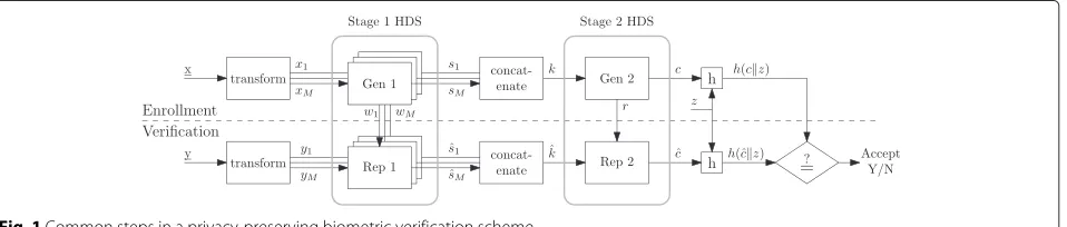
Figure 1 shows the data flow and processing steps in the two-stage helper data scheme. In a preparation phase preceding all enrollments, the population’s biometrics are studied and a transform is derived (using well known techniques such as principal component analysis or lin-ear discriminant analysis [13]). The transform splits the biometric vector x into scalar components (xi)Mi=1. We will refer to these componentsxi as features. The
trans-form ensures that they are mutually independent, or nearly so.
At enrollment, a person’s biometric x is obtained. The transform is applied, yielding features (xi)Mi=1. The Gen algorithm of the first-stage HDS is applied to each feature independently. This gives continuous helper data(wi)Mi=1 and short secret strings s1,. . .,sM which may or may
not have equal length, depending on the signal-to-noise ratio of the features. All these secrets are combined into one high-entropy secret k, e.g., by concatenating them after Gray-coding. Biometric features are subject to noise, which will lead to some errors in the reproduced secret
ˆ
k; hence, a second stage of error correction is done with another HDS. The output of the second-stageGen algo-rithm is discrete helper datarand a practically noiseless string c. The hash h(cz) is stored in the enrollment database, along with the helper data(wi)Mi=1andr. Here ,z is salt, a random string to prevent easy cross-matching.
In the authentication phase, a fresh biometric measure-ment y is obtained and split into components (yi)Mi=1.
For each i independently, the estimator ˆsi is computed
from yi and wi. The ˆsi are combined into an
estima-tor kˆ, which is then input into the 2nd-stage HDS reconstruction together with r. The result is an esti-mator ˆc. Finally, h(cˆz) is compared with the stored hashh(cz).
1.4 Fuzzy extractors and secure sketches
Special algorithms have been developed for HDSs [4, 6, 8, 9]: Fuzzy extractors (FE) and secure sketches (SS). The FE and SS are special cases of the general HDS concept. They have different requirements,
• Fuzzy extractor
The probability distribution ofs given w has to be (nearly) uniform.
• Secure sketch
s given w must have high entropy, but does not have to be uniform. Typically,s is equal to (a discretized version of)x.
The FE is typically used for the extraction of crypto-graphic keys from noisy sources such as physical unclon-able functions (PUFs) [14–16]. Some fixed quantization schemes support the use of a fuzzy extractor, provided that the quantization intervals can be chosen such that each secretsis equiprobable, as in [17].
The SS is very well suited to the biometrics scenario described above.
1.5 Security and privacy
In the HDS context, the main privacy question is how much information, andwhichinformation, about the bio-metric x is leaked by the helper data. Ideally, the helper data would contain just enough information to enable the error correction. Roughly speaking, this means that the vector w=(wi)Mi=1consists of the noisy “least significant
bits” of x, which typically do not reveal sensitive informa-tion since they are noisy anyway. In order to make this kind of intuitive statement more precise, one studies the information-theoretic properties of HDSs. In the system as sketched in Fig. 1, the mutual information1I(C; W,R)
is of particular interest: it measures the leakage about the stringccaused by the fact that the attacker observes w and
r. By properly separating the “most significant digits” of x from the “least significant digits”, it is possible to achieve
I(C; W,R)=0. We call this zero secrecy leakage or, more compactly, zero leakage (ZL).2HDSs with the ZL property are very interesting for quantifying privacy guarantees: if a privacy-sensitive piece of a biometric is fully contained in
c, and not in(w,r), then a ZL HDS based database reveals
absolutely nothingabout that piece.3
We will focus in particular on schemes whose first stage has the ZL property for each feature separately:
I(Si;Wi)=0. If the transform in Fig. 1 yields independent
features, then automaticallyI(Sj;Wi) = 0 for alli,j, and
the whole first stage has the ZL property.
1.6 Contributions and organization of this paper
In this paper, we zoom in on the first-stage HDS and focus on the ZL property in particular. Our aim is to minimize
reconstruction errors in ZL HDSs that have scalar input
x ∈ R. We treat the helper data as being real-valued,
w ∈ R, though of course w is in practice stored as a finite-precision value.
• We show that the ZL constraint for continuous helper data necessitates the existence of “Sibling Points”, pointsx that correspond to different s but give rise to the same helper dataw.
• We prove that the ZL constraint forx∈Rimplies “quantile” helper data. This holds for uniformly distributeds as well as for non-uniform s. Thus, we identify a simple quantile construction as being the generic ZL scheme for all HDS types, including the FE and SS as special cases. It turns out that the continuum limit of a FE scheme of Verbitskiy et al. [7] precisely corresponds to our quantile HDS.
• We derive a reconstruction algorithm for the quantile ZL FE that minimizes the reconstruction errors. It amounts to using a set of optimized threshold values, and is very suitable for low-footprint implementation.
• We analyze, in an all-Gaussian example, the performance (in terms of reconstruction error rate) of our ZL FE combined with the optimal
reconstruction algorithm. We compare this scheme to fixed quantization and a likelihood-based classifier. It turns out that our error rate is better than that of fixed quantization, and not much worse than that of the likelihood-based classifier.
The organization of this paper is as follows. Section 2 discusses quantization techniques. After some preliminar-ies (Section 3), the sibling points and the quantile helper data are treated in Section 4. Section 5 discusses the opti-mal reconstruction thresholds. The performance analysis in the Gaussian model is presented in Section 6.
2 Related work on biometric quantization
Many biometric parameters can be converted by a principal component analysis (PCA) into a vector of (near)independent components [18]. For this reason, most papers on helper data in the analog domain can restrict themselves to a one-dimensional quantization, e.g., [4, 6, 18]. Yet, the quantization strategies differ, as we will review below. Figure 2 shows the probability density function (PDF) of the measurement y in the verifica-tion phase and how the choice of quantizaverifica-tion regions in the verification phase affects the probability of erroneous reconstruction (shaded area) in the various schemes.
2.1 Fixed quantization (FQ)
a b c
Fig. 2Examples of adaptating the genuine user PDF in the verification phase. FQ does not translate the PDF; QIM centers the PDF on a quantization interval; LQ uses a likelihood ratio to adjust the quantization regions.aFixed equiprobable quantization.bQuantization Index Modulation.
cMulti-bits based on likelihood ratio [6]
in Fig. 2a. An unfavorably located genuine user pdf, near a quantization boundary, can cause a high reconstruction error.
The inherently large error probability can be mitigated by “reliable component” selection [17]. Only components
xi far away from a boundary are selected; the rest are
discarded. The indices of the reliable components consti-tute the helper data. Such a scheme is very inefficient, as it wastes resources: features that are unfavorably located w.r.t. the quantization grid, but nonetheless carry infor-mation, are eliminated. Furthermore, the helper data leaks information about the biometric, since the intervals have unequal width and therefore unequal probabilities of pro-ducing reliable components [19].
2.2 Quantization index modulation (QIM)
QIM borrows principles from digital watermarking [20] and writing on dirty paper [21]. QIM has quantization intervals alternatingly labeled with ‘s‘0” and “1” as the val-ues for the secrets. The helper datawis constructed as the distance fromxto the middle of a quantization inter-val; adding wto ythen offsets the pdf so that the pdf is centered on the interval (Fig. 2b), yielding a significantly lower reconstruction error probability than FQ.
The freedom to choose quantization step sizes allows for a trade-off between reconstruction performance and leakage [4]. The alternating labeling was adopted to reduce leakage but sacrifices a large part of the source’s entropy.
2.3 Likelihood-based quantization (LQ)
At enrollment, the LQ scheme [6] allocates N quanti-zation regions as follows. The first two boundaries are chosen such that they yield the same probability of y
givenx, and at the same time enclose a probability mass 1/N on the background distribution (the whole popula-tion’s distribution). Subsequent quantization intervals are
chosen contiguous to the first and again enclose a 1/N
probability mass. Finally, the probability mass in the tails of the background distribution is added up as a wrap-around interval, which also holds a probability mass of 1/N. Since the quantization boundaries are at fixed prob-ability mass intervals, it suffices to communicate a single boundarytas helper data to the verification phase.
In LQ, the secretsis not equiprobable. The error rates are low, but the revealedtleaks information abouts.
2.4 Dynamic detection-rate-based bit allocation
In [22], Lim et al. proposed dynamic genuine interval search (DGIS) as an improvement of the bit allocation scheme of Chen et al. [23]. The resulting scheme has some similarity to our approach in that they both determine discretization intervals per user and store these inter-vals as helper data. However, their scheme is motivated solely by optimization of the detection rate, whereas in our scheme the optimization is subject to the zero leakage restriction. Applying the DGIS method introduces some additional leakage to the underlying bit allocation scheme. Furthermore, DGIS performs its search for the optimal discretization intervals using a sliding window algorithm, which in general will not succeed in finding the exact opti-mum. In contrast, in our scheme, we analytically derive the optimal solution from the background distribution.
3 Preliminaries 3.1 Notation
Random variables are denoted with capital letters and their realizations in lowercase. The notationEstands for expectation. Sets are written in calligraphic font. We zoom in on the one-dimensional first-stage HDS in Fig. 1. For brevity of notation the indexi∈ {1,. . .,M}onxi,wi,si,yi
andsˆiwill be omitted.
asfA, and the cumulative distribution function (CDF) as FA. We considerX ∈ R. The helper data is considered
continuous, W ∈ W ⊂ R. Without loss of generality we fixW =[ 0, 1). The secretSis an integer in the range
S = {0,. . .,N−1}, whereN is a system design choice, typically chosen according to the signal to noise ratio of the biometric feature. The helper data is computed from
Xusing a functiong, i.e.,W =g(X). Similarly, we define a quantization functionQsuch thatS= Q(X). The enroll-ment part of the HDS is given by the pairQ,g. We define quantization regions as follows,
As= {x∈R:Q(x)=s}. (1)
The quantization regions are non-overlapping and cover the complete feature space, hence form a partitioning:
As∩At= ∅ fors=t;
s∈S
As=R. (2)
We consider only quantization regions that are contigu-ous, i.e., for alls it holds thatAs is a simple interval. In
Section 5.3, we will see that many other choices may work equally well,but not better; our preference for contiguous
As regions is tantamount to choosing the simplest
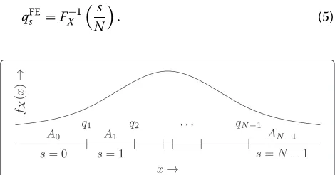
ele-mentQout of a whole equivalence class of quantization functions that lead to the same HDS performance. We define quantization boundariesqs = infAs. Without loss
of generality, we chooseQto be a monotonically increas-ing function. This gives supAs=qs+1. An overview of the quantization regions and boundaries is depicted in Fig. 3. In a generic HDS, the probabilitiesP[S = s] can be different for eachs. We will use shorthand notation
P[S=s]=ps>0. (3)
The quantization boundaries are given by
qs=FX−1
whereFX−1is the inverse CDF. For a Fuzzy extractor, one requiresps=1/Nfor alls, in which case (4) simplifies to
Fig. 3Quantization regionsAsand boundariesqs. The locations of
the quantization boundaries are based on the distribution ofx, such that secretsoccurs with probabilityps
3.2 Zero leakage
We will work with a definition of the zeroleakage prop-erty that is a bit stricter than the usual formulation [7], which pertains to mutual information. This is necessary in order to avoid problems caused by the fact thatW is a continuum variable (e.g., pathological cases where some property does not hold on measure-zero subsets ofW),
Definition 3.1. We call a helper data schemeZero Leak-ageif and only if
∀V⊆W P[S=s|W ∈V]=P[S=s] . (6)
In words, we define the ZL property as independence betweenSandW. Knowledge aboutW has no effect on the adversary’s uncertainty aboutS. ZL impliesI(S;W)=
0 or, equivalently, H(S|W) = H(S). Here H stands for Shannon entropy, andIfor mutual information (see, e.g., ([24], Eq. (2.35)–(2.39)).
3.3 Noise model
It is common to assume a noise model in which the enroll-ment measureenroll-mentxand verification measurementyare both derived from a hidden ‘true’ biometric valuez, i.e.,
X = Z + Ne and Y = Z + Nv, whereNe stands for the noise in the enrollment measurement andNvfor the noise in the verification measurement. It is assumed that
NeandNvare mutually independent and independent of
XandY. TheNe,Nvhave zero mean and varianceσe2,σv2 respectively. The variance ofz is denoted asσZ2. This is a very generic model. It allows for various special cases such as noiseless enrollment, equal noise at enrollment, and verification, etc.
It is readily seen that the variance ofX andY is given by σX2 = σZ2 + σe2 and σY2 = σZ2 + σv2. The correla-tion coefficient ρ betweenX and Y is defined as ρ =
(E[XY]−E[X]E[Y])/(σXσY)and it can be expressed as
whereRis zero-mean noise. This way of expressingY is motivated by the first and second order statistics, i.e., the variance of Y is λ2σX2 +σ2 = σY2, and the correlation betweenXandYisE[XY]/(σXσY)=λσX2/(σXσY)=ρ.
In the case of Gaussian Z,Ne,Nv, the X and Y are Gaussian, and the noiseRis Gaussian as well.
From (7), it follows that the PDF ofygivenx(i.e., the noise between enrollment and verification) is centered on
λx and has variance σ2. The parameter λ is called the attenuation parameter. In the “identical conditions” case
“noiseless enrollment” caseσe = 0 we haveλ = 1 and
ρ=σZ/
σ2 Z+σv2.
We will adopt expression (7) as our noise model. In Section 5.1, we will be considering a class of noise distributions that we callsymmetric fading noise.
Definition 3.2. Let X be the enrollment measurement and let Y be the verification measurement, where we adopt be model of Eq. (7). Let fY|X denote the probability density function of Y given X. The noise is calledsymmetric fading noiseif for all x,y1,y2it holds that
|y1−λx|<|y2−λx| =⇒ fY|X(y1|x) >fY|X(y2|x). (8)
Equation (8) reflects the property that small noise excursions are more likely than large ones, and that the sign of the noise is equally likely to be positive or neg-ative. Gaussian noise is an example of symmetric fading noise.
4 Zero leakage: quantile helper data
In Section 4.1, we present a chain of arguments from which we conclude that, for ZL helper data, it is sufficient to consider only functionsgwith the following properties: (1) coveringWon each quantization interval (surjective); (2) monotonically increasing on each quantization inter-val. This is then used in Section 4.2 to derive the main result, Theorem 4.8: Zero Leakage is equivalent to hav-ing helper data obeyhav-ing a specific quantile rule. This rule makes it possible to construct a very simple ZL HDS which is entirely generic.
4.1 Why it is sufficient to consider monotonically increasing surjective functionsg
The reasoning in this section is as follows. We define sib-ling pointsas pointsxin different quantization intervals but with equalw. We first show that for every w, there must be at least one sibling point in each interval (surjec-tivity); then, we demonstrate that having more than one is bad for the reconstruction error rate. This establishes that each interval must contain exactly one sibling point for each w. Then, we show that the ordering of sibling points must be the same in each interval, because oth-erwise the error rate increases. Finally, assuminggto be differentiable yields the monotonicity property.
The verifier has to reconstructxbased onyandw. In general this is done by first identifying which pointsx ∈ Rare compatible withw, and then selecting which one is most likely, givenyandw. For the first step, we introduce the concept ofsibling points.
Definition 4.1.(Sibling points): Two points x,x ∈ R, with x=x, are called Sibling Points if g(x)=g(x).
The verifier determines a setXw = {x ∈ R|g(x) = w}
of sibling points that correspond to helper data valuew. We write Xw = ∪s∈SXsw, withXsw = {x ∈ R|Q(x) = s∧g(x)=w}. We derive a number of requirements on the setsXsw.
Lemma 4.2. ZL implies that
∀w∈W,s∈S Xsw= ∅. (9)
Proof: see Appendix A1. Lemma 4.2 tells us that there is significant leakage if there is not at least one sibling point compatible withwin each intervalAs, for allw∈W. Since
we are interested in zero leakage, we will from this point onward consider only functionsgsuch thatXsw = ∅for
alls,w.
Next, we look at the requirement of low reconstruc-tion error probability. We focus on theminimum distance
between sibling points that belong to different quantiza-tion intervals.
Definition 4.3. The minimum distance between sibling points in different quantization intervals is defined as
Dmin(w)= min
s,t∈S:s<t|minXtw−maxXsw|, (10) Dmin= min
w∈WDmin(w). (11)
We take the approach of maximizing Dmin. It is intu-itively clear that such an approach yields low error rates given the noise model introduced in Section 3.3. The following lemma gives a constraint that improves theDmin.
Lemma 4.4. Let w∈ WandXsw= ∅for all s∈S. The Dmin(w)is maximized by setting|Xsw| =1for all s∈S.
Proof: see Appendix A.2. Lemma 4.4 states that each quantization intervalAsshould contain exactly one point x compatible with w. From here onward we will only consider functionsgwith this property.
The set Xsw consists of a single point which we will
denote as xsw. Note that g is then an invertible
func-tion on each interval As. For given w ∈ W, we now
have a set Xw = ∪s∈Sxsw that consists of one
sib-ling point per quantization interval. This vastly simplifies the analysis. Our next step is to put further constraints ong.
Lemma 4.5. Let x1,x2∈ Asand x3,x4 ∈At, s =t, with x1<x2<x3<x4and g(x1)=w1, g(x2)=w2. Consider
1. g(x3)=w1; g(x4)=w2
Proof: see Appendix A.3. Lemma 4.5 tells us that the ordering of sibling points should be the same in each quantization interval, for otherwise the overall minimum distanceDminsuffers. If, for somes, a pointxwith helper dataw2is higher than a point with helper dataw1, then this order has to be the same for all intervals.
The combination of having a preserved order (Lemma 4.5) together with g being invertible on each interval (Lemma 4.4) points us in the direction of “smooth” functions. Ifg is piecewise differentiable, then we can formulate a simple constraint as follows.
Theorem 4.6.(sign ofg’ equal on each As) : Let xs ∈
If we consider a function g that is differentiable on each quantization interval, then (1) its piecewise invert-ibility implies that it has to be either monotonously increasing or monotonously decreasing on each inter-val, and (2) Theorem 4.6 then implies that it has to be either increasing on all intervals or decreasing on all intervals.
Of course there is no reason to assume thatgis piece-wise differentiable. For instance, take a piecepiece-wise differ-entiable g and apply a permutation to the w-axis. This procedure yields a function g2 which, in terms of error probabilities, has exactly the same performance asg, but is not differentiable (nor even continuous). Thus, there exist huge equivalence classes of helper data generating functions that satisfy invertibility (Lemma 4.4) and proper ordering (Lemma 4.5). This brings us to the following con-jecture, which allows us to concentrate on functions that are easy to analyze.
Conjecture 4.7. Without loss of generality we can choose the function g to be differentiable on each quantization interval As, s∈S.
Based on Conjecture 4.7, we will consider only functions
gthat are monotonicallyincreasingon each interval. This assumption is in line with all (first stage) HDSs [4, 6, 8] known to us.
4.2 Quantile helper data
We state our main result in the theorem below.
Theorem 4.8.(ZL is equivalent to quantile
relation-ship between sibling points): Let g be monotonously
increasing on each interval As, with g(A0) = · · · =
g(AN−1) = W. Let s,t ∈ S. Let xs ∈ As,xt ∈ At be sib-ling points as defined in Def. 4.1. In order to satisfy Zero Leakage we have the following necessary and sufficient condition on the sibling points,
FX(xs)−FX(qs)
Corollary 4.9. (ZL FE sibling point relation): Let g be monotonously increasing on each interval As, with g(A0)= · · · = g(AN−1) = W. Let s,t ∈ S. Let xs ∈ As,xt ∈ At be sibling points as defined in Def. 4.1. Then for a Fuzzy Extractor we have the following necessary and sufficient condition on the sibling points in order to satisfy Zero Leakage,
Proof.Immediately follows by combining Eq. (13) with the fact thatps = 1/N ∀s ∈ Sin a FE scheme, and with
the FE quantization boundaries given in Eq. (5).
Theorem 4.8 allows us to define the enrollment steps in a ZL HDS in a very simple way,
data can be interpreted as a quantile distance between
x and the quantization boundary qs, normalized with
respect to the probability massps in the intervalAs. An
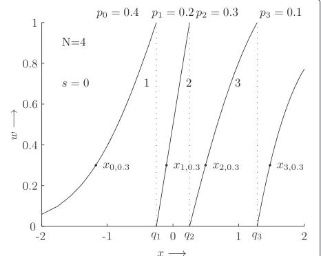
example of such a function is depicted in Fig. 4. For a spe-cific distribution, e.g., a standard Gaussian distribution, the helper data generation function is depicted in Fig. 5. In the FE case, Eq. (15) simplifies to
FX(x)= s+w
N ; w∈[ 0, 1) (16)
and the helper data generation function becomes
w=gFE(x)=N·FX(x)−s. (17)
Fig. 4Example of helper data generating functiongforN=4 on quantilex, i.e.,FX(x). The probabilities of the secrets do not have to be
equal; in this case, we have used(p0,. . .,p3)=(0.4, 0.2, 0.3, 0.1)
an enrollment that satisfies the sibling point relation of Theorem 4.8. However, it is not theonlyway. For instance, by applying any invertible function tow, a new helper data scheme is obtained that also satisfies the sibling point rela-tion (13) and hence is ZL. Another example is to store the whole set of sibling points{xtw}t∈S; this contains exactly the same information asw. The transformed scheme can be seen as merely a different representation of the “basic” ZL HDS (15). Such a representation may have various advantages over (15), e.g., allowing for a faster recon-struction procedure, while being completely equivalent in terms of the ZL property. We will see such a case in Section 5.3.
Fig. 5Example of a helper data generating functiongfor a standard Gaussian distribution, i.e.,x∼N(0, 1), andN=4. Sibling pointsxsw
are given fors∈ {0,. . ., 3}andw=0.3
5 Optimal reconstruction
5.1 Maximum likelihood and thresholds
The goal of the HDS reconstruction algorithm Rep(y,w)
is to reliably reproduce the secret s. The best way to achieve this is to choose the most probablesˆgivenyandw, i.e., a maximum likelihood algorithm. We derive optimal decision intervals for the reconstruction phase in a Zero Leakage Fuzzy Extractor.
Lemma 5.1. LetRep(y,w)be the reproduction algorithm of a ZL FE system. Let g−s1 be the inverse of the helper data generation function for a given secret s. Then optimal reconstruction is achieved by
Rep(y,w)=arg max
s∈S fY|X
y|g−s1(w) . (18)
Proof: see Appendix A.6. To simplify the verification phase we can identify thresholdsτsthat denote the lower
boundary of a decision region. Ifτs≤y< τs+1, we recon-structˆs=s. Theτ0 = −∞andτN = ∞are fixed, which
implies we have to find optimal values only for theN−1 variablesτ1,. . .,τN−1as a function ofw.
Theorem 5.2. Let fY|X represent symmetric fading noise. Then optimal reconstruction in a FE scheme is obtained by the following choice of thresholds
τs=λ
gs−1(w)+gs−−11(w)
2 . (19)
Proof. In case of symmetric fading noise we know that
fY|X(y|x)=ϕ(|y−λx|), (20)
withϕsome monotonic decreasing function. Combining this notion with that of Eq. (18) to find a pointy=τsthat
gives equal probability forsands−1 yields
ϕ|τs−λgs−−11(w)|
=ϕ|τs−λgs−1(w)| . (21)
The left and right hand side of this equation can only be equal for equal arguments, and hence
τs−λgs−−11(w)= ±
τs−λgs−1(w) . (22)
Since gs−1(w) = gs−−11(w) the only viable solution is Eq. (19).
Instead of storing the ZL helper data w according to (15), one can also store the set of thresholdsτ1,. . .,τN−1. This contains precisely the same information, and allows for quicker reconstruction ofs: just a thresholding opera-tion onyand theτsvalues, which can be implemented on
5.2 Special case: 1-bit secret
In the case of a one-bit secret s, i.e., N = 2, the above ZL FE scheme is reduced to storing a single thresholdτ1.
It is interesting and somewhat counterintuitive that this yields a threshold for verification that does not leak infor-mation about the secret. In case the average ofXis zero, one might assume that a positive threshold value implies
s = 0. However, boths = 0 ands = 1 allow positive as well as negativeτ1, dependent on the relative location ofx in the quantization interval.
5.3 FE: equivalent choices for the quantization
Let us reconsider the quantization functionQ(x) in the case of a Fuzzy extractor. Let us fixNand take the g(x)
as specified in Eq. (16). Then, it is possible to find an infi-nite number of different functionsQthat will conserve the ZL property and lead to exactly the same error rate as the original scheme. This is seen as follows. For anyw∈[ 0, 1), there is anN-tuplet of sibling points. Without any impact on the reconstruction performance, we can permute the
s-values of these points; the error rate of the reconstruc-tion procedure depends only on thex-values of the sibling points, not on thes-label they carry. It is allowed to do this permutation for everywindependently, resulting in an infinite equivalence class of Q-functions. The choice we made in Section 3 yields the simplest function in an equivalence class.
6 Example: Gaussian features and BCH codes
To benchmark the reproduction performance of our scheme, we give an example based on Gaussian-distributed variables. In this example, we will assume all variables to be Gaussian distributed, though we remind
the reader that our scheme specifies optimal reconstruc-tion thresholds even for non-Gaussian distribureconstruc-tions.
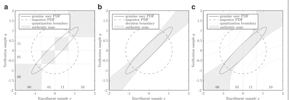
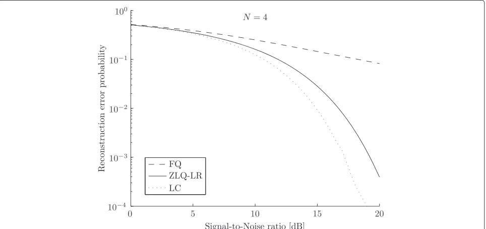
We compare the reproduction performance of our ZL quantization scheme with Likelihood-based reproduction (ZLQ-LR) to a scheme with (1) fixed quantization (FQ), see Section 2.1, and (2) likelihood classification (LC). The former is, to our knowledge, the only other scheme shar-ing the zero secrecy leakage property, since it does not use any helper data. An example with N = 4 intervals is depicted in Fig. 6a. LC is not an actual quantization scheme since it requires the enrollment sample to be stored in-the-clear. However, a likelihood based classifier provides an optimal trade-off between false acceptance and false rejection according to communication theory [24] and should therefore yield the lowest possible error rate. Instead of quantization boundaries, the classifier is characterized by decision boundaries as depicted in Fig. 6b.
A comparison with QIM cannot be made since there the probability for an impostor to guess the enrolled secret cannot be made equal to 1/N. This would result in an unfair comparison since the other schemes are designed to possess this property. Moreover, the QIM scheme allows the reproduction error probability to be made arbitrary small by increasing the quantization width at the cost of leakage.
Also, the likelihood based classification can be tuned by setting the decision threshold. However, for this scheme, it is possible to choose a threshold such that an impostor will have a probability of 1/Nto be accepted, which cor-responds to the 1/N probability of guessing the enrolled secret in a FE scheme. Note that for a likelihood classifier, there is no enrolled secret since this is not a quantization scheme.
a
b
c
Fig. 6Quantization and decision patterns based on the genuine user and impostor PDFs. Ideally the genuine user PDF should be contained in the authentic zone and the impostor PDF should have a large mass outside the authentic zone. Fifty percent probability mass is contained in the genuine user and impostor PDF ellipse and circle. The genuine user PDF is based on a 10 dB SNR.aFixed equiprobable quantization (FQ).
As can be seen from Fig. 7, the reproduction perfor-mance for a ZL scheme with likelihood based reproduc-tion is always better than that of a fixed quantizareproduc-tion scheme. However, it is outperformed by the likelihood classifier. Differences are especially apparent for features with a higher signal-to-noise ratio. In these regions, the fixed quantization struggles with a inherent high error probability, while the ZL scheme follows the LC.
In a good quantization scheme, the gap betweenI(X;Y)
and I(S;Sˆ) must be small. For a Gaussian channel, standard expressions are known from ([24], Eq. (9.16)). Figure 8 shows that a fixed quantization requires a higher SNR on order to converge to the maximum number of bits, whereas the ZLQ-LR scheme directly reaches this value.
Finally, we consider the vector case of the two quanti-zation schemes discussed above. We concluded that FQ has a larger error probability, but we now show how this relates to either false rejection or secret length when combined with a code offset method [3].
We assume i.i.d. features and therefore we can calculate false acceptance rate (FAR) and false rejection rate (FRR) based on a binomial distribution. In practice, features can be made (nearly) independent, but they will in general not be identically distributed. However, results will be simi-lar. Furthermore we assume the error correcting code can be applied such that its error correcting properties can be fully exploited. This implies that we have to use a Gray code to label the extracted secrets before concatenation.
We used 64 i.i.d. features, each having a SNR of 17 dB, which is a typical average value for biometric features
[8, 17]. From these features, we extract 2 bits per feature on which we apply BCH codes with a code length of 127. (We omit one bit). For analysis, we have also included the code (127, 127, 0), which is not an actual code, but represents the case in which no error correction is applied. Suppose we want to achieve a target FRR of 1·10−3, the topmost dotted line in Fig. 9, then we require a BCH (127, 92, 5) code for the ZLQ-LR scheme, while a BCH (127, 15, 27) code is required for the FQ scheme. This implies that we would have a secret key size of 92 bits versus 15 bits. Clearly, the latter is not sufficient for any security application. At the same time, due to the small key size, FQ has an increased FAR.
7 Conclusions
In this paper, we have studied a generic helper data scheme (HDS) which comprises the Fuzzy extractor (FE) and the secure sketch (SS) as special cases. In particular, we have looked at the zero leakage (ZL) property of HDSs in the case of a one-dimensional continuous sourceXand continuous helper dataW.
We make minimal assumptions, justified by Conjecture 4.7: we consider only monotonicg(x). We have shown that the ZL property implies the existence of sibling points {xsw}s∈S for everyw. These are values ofxthat have the
same helper data w. Furthermore, the ZL requirement is equivalent to a quantile relationship (Theorem 4.8) between the sibling points. This directly leads to Eq. (15) for computing wfrom x. (Applying any reversible func-tion to thiswyields a completely equivalent helper data
Fig. 8Mutual information betweenSandˆSfor Gaussian-distributed features and Gaussian noise
system.) The special case of a FE (ps = 1/N) yields the m→ ∞limit of the Verbitskiy et al. [7] construction.
We have derived reconstruction thresholds τs for a
ZL FE that minimize the error rate in the reconstruc-tion of s (Theorem 5.2). This result holds under very mild assumptions on the noise: symmetric and fad-ing. Equation (19) contains the attenuation parameter
λ, which follows from the noise model as specified in Section 3.3.
Finally, we have analyzed reproduction performance in an all-Gaussian example. Fixed quantization struggles with inherent high error probability, while the ZL FE with optimal reproduction follows the performance of the optimal classification algorithm. This results in a larger key size in the protected template compared to the fixed quantization scheme, since an ECC with a larger message length can be applied in the second stage HDS to achieve the same FRR.
In this paper, we have focused on arbitrary but known probability densities. Experiments with real data are beyond the scope of this paper, but have been reported in [26, 27]. A key finding there was that modeling the distributions can be problematic, especially due to sta-tistical outliers. Even so, improvements were obtained with respect to earlier ZL schemes. We see modeling refinements as a topic for future research.
Endnotes
1For information-theoretic concepts such as Shannon
entropy and mutual information we refer to e.g. [24].
2This concept is not new. Achieving zero mutual
information has always been a (sometimes achievable) desideratum in the literature on fuzzy vaults/fuzzy extractors/secure sketches for discrete and continuous sources.
3An overall Zero-Leakage scheme can be obtained in
the final HDS stage even from a leaky HDS by applying privacy amplification as a post-processing step. However, this procedure discards substantial amounts of source entropy, while in many practical applications it is already a challenge to achieve reasonable security levels from biometrics without privacy protection.
Appendix
Appendix A: Proofs A.1 Proof of Lemma 4.2
Pick anyw∈W. The statementw∈Wmeans that there exists at least ones∈Ssuch thatXsw= ∅. Now suppose
there exists somes∈SwithXsw= ∅. Then knowledge
ofwreveals information aboutS, i.e.P[S = s|W = w]=
P[S=s], which contradicts ZL.
A.2 Proof of Lemma 4.4
Letgbe such that|Xsw|>1 for somes,w. Then choose a
A.3 Proof of Lemma 4.5
We tabulate the Dmin(w) values for case 1 and 2, case 1 case 2
w1 x3−x1 x4−x1
w2 x4−x2 x3−x2
The smallest of these distances isx3−x2.
A.4 Proof of Theorem 4.6
Let 0< ε1 and 0< δ 1. Without loss of generality we considers < t. We invoke Lemma 4.5 withx1 = xs,
x2=xs+ε,x3=xt,x4=xt+δ. According to Lemma 4.5
we have to takeg(x2) = g(x4)in order to obtain a large
Dmin. Applying a first order Taylor expansion, this gives
g(xs)+εg(xs)+O(ε2)=g(xt)+δg(xt)+O(δ2). (24)
We use the fact thatg(xs) =g(xt), and thatεandδare
positive. Taking the sign of both sides of (24) and neglect-ing second order contributions, we get sign g(xs) =
signg(xt).
A.5 Proof of Theorem 4.8
The ZL property is equivalent tofW = fW|S, which gives function on each intervalAs, fully spanningW. Then for
givensandwthere exists exactly one pointxswthat
satis-fiesQ(x)=sandg(x)=w. Furthermore, conservation of probability then givesfW,S(w,s)dw = fX(xsw)dxsw. Since
the right hand side of (25) is independent ofs, we can write
fW(w)dw= p−s1fX(xsw)dxswforany s ∈S. Hence for any
which can be rewritten as
dFX(xsw) ps =
dFX(xtw) pt
. (27)
The result (13) follows by integration, using the fact that
Ashas lower boundaryqs.
A.6 Proof of Lemma 5.1
Optimal reconstruction can be done by selecting the most likely secret giveny,w,
The denominator does not depend ons, and can hence be omitted. This gives
Rep(y,w)=arg max
s∈S fS,Y,W(s,y,w) (29)
=arg max
s∈S fY|S,W(y|s,w)fW|S(w|s)ps. (30)
We constructed the scheme to be a FE with ZL, and thereforeps = 1/N andfW|S(w|s) = fW(w). We see that
bothpsandfW|S(w|s)do not depend ons, which implies
they can be omitted from Eq. (30), yielding Rep(y,w) =
equivalent to knowing X. Hence fY|S,W(y|s,w) can be
replaced byfY|X(y|x)withxsatisfyingQ(x)=sandg(x)= w. The unique xvalue that satisfies these constraints is
gs−1(w).
Competing interests
The authors declare that they have no competing interests.
Author details
1Signal Processing Systems group, Department of Electrical Engineering, Eindhoven University of Technology, 5600 MB, Eindhoven, The Netherlands. 2Security and Embedded Networked Systems group, Department of Mathematics and Computer Science, Eindhoven University of Technology, 5600 MB Eindhoven, The Netherlands.3Discrete Mathematics group, Department of Mathematics and Computer Science, Eindhoven University of Technology, 5600 MB Eindhoven, The Netherlands.4Genkey Solutions B.V., High Tech Campus 69, 5656 AG Eindhoven, The Netherlands.
Received: 22 October 2015 Accepted: 20 April 2016
References
1. T van der Putte, J Keuning, inProceedings of the Fourth Working Conference on Smart Card Research and Advanced Applications on Smart Card Research and Advanced Applications. Biometrical fingerprint recognition: don’t get your fingers burned (Kluwer Academic Publishers, Norwell, MA, USA, 2001), pp. 289–303
2. T Matsumoto, H Matsumoto, K Yamada, S Hoshino, Impact of artificial “gummy” fingers on fingerprint systems. Opt. Secur. Counterfeit Deterrence Tech.4677, 275–289 (2002)
3. A Juels, M Wattenberg, inCCS ’99: Proceedings of the 6th ACM Conf on Comp and Comm Security. A fuzzy commitment scheme (ACM, New York, NY, USA, 1999), pp. 28–36. doi:10.1145/319709.319714. http://doi.acm. org/10.1145/319709.319714
4. J-P Linnartz, P Tuyls, inNew Shielding Functions to Enhance Privacy and Prevent Misuse of Biometric Templates, ed. by J Kittler, Mark Nixon. Audio-and Video-Based Biometric Person Authentication: 4th International Conference, AVBPA 2003 Guildford, UK, June 9–11, 2003 Proceedings (Springer Berlin Heidelberg, Berlin, Heidelberg, 2003), pp. 393–402. doi:10.1007/3-540-44887-X_47. http://dx.doi.org/10.1007/3-540-44887-X_47
5. P Tuyls, B Škori´c, T Kevenaar,Security with Noisy Data: Private
Biometrics, Secure Key Storage and Anti-Counterfeiting. (Springer, Secaucus, NJ, USA, 2007)
6. C Chen, RNJ Veldhuis, TAM Kevenaar, AHM Akkermans, inProc. IEEE Int. Conf. on Biometrics: Theory, Applications, and Systems. Multi-bits biometric string generation based on the likelihood ratio (IEEE, Piscataway, 2007) 7. EA Verbitskiy, P Tuyls, C Obi, B Schoenmakers, B Škori´c, Key extraction
from general nondiscrete signals. Inform. Forensics Secur. IEEE Trans.5(2), 269–279 (2010)
8. JA de Groot, J-PMG Linnartz, inProc. IEEE Int. Conf. Acoust., Speech, Signal Process. Zero leakage quantization scheme for biometric verification, (Piscataway, 2011)
9. Y Dodis, L Reyzin, A Smith, inFuzzy Extractors: How to Generate Strong Keys from Biometrics and Other Noisy Data, ed. by C Cachin, JL Camenisch. Advances in Cryptology - EUROCRYPT 2004: International Conference on the Theory and Applications of Cryptographic Techniques, Interlaken, Switzerland, May 2-6, 2004. Proceedings (Springer Berlin Heidelberg, Berlin, Heidelberg, 2004), pp. 523–540. doi:10.1007/978-3-540-24676-3_31 http://dx.doi.org/10.1007/978-3-540-24676-3_31
10. AV Herrewege, S Katzenbeisser, R Maes, R Peeters, A-R Sadeghi, I Verbauwhede, C Wachsmann, inReverse Fuzzy Extractors: Enabling Lightweight Mutual Authentication for PUF-Enabled RFIDs, ed. by AD Keromytis. Financial Cryptography and Data Security: 16th International Conference, FC 2012, Kralendijk, Bonaire, Februray 27-March 2, 2012, Revised Selected Papers (Springer Berlin Heidelberg, Berlin, Heidelberg, 2012), pp. 374–389. doi:10.1007/978-3-642-32946-3_27. http://dx.doi.org/ 10.1007/978-3-642-32946-3_27
11. B Škori´c, N de Vreede, The spammed code offset method. IEEE Trans. Inform. Forensics Secur.9(5), 875–884 (2014)
12. F MacWilliams, N Sloane,The Theory of Error Correcting Codes. (Elsevier, Amsterdam, 1978)
13. JL Wayman, AK Jain, D Maltoni, D Maio (eds.),Biometric Systems: Technology, Design and Performance Evaluation, 1st edn. (Spring Verlag, London, 2005)
14. B Škori´c, P Tuyls, W Ophey, inRobust Key Extraction from Physical Uncloneable Functions, ed. by J Ioannidis, A Keromytis, and M Yung. Applied Cryptography and Network Security: Third International Conference, ACNS 2005, New York, NY, USA, June 7-10, 2005. Proceedings (Springer Berlin Heidelberg, Berlin, Heidelberg, 2005), pp. 407–422. doi:10.1007/11496137_28. http://dx.doi.org/10.1007/11496137_28 15. GE Suh, S Devadas, inProceedings of the 44th Annual Design Automation
Conference.DAC ’07. Physical unclonable functions for device authentication and secret key generation (ACM, New York, NY, USA, 2007), pp. 9–14
16. DE Holcomb, WP Burleson, K Fu, Power-Up SRAM state as an identifying fingerprint and source of true random numbers. Comput. IEEE Trans.
58(9), 1198–1210 (2009)
17. P Tuyls, A Akkermans, T Kevenaar, G-J Schrijen, A Bazen, R Veldhuis, in
Practical Biometric Authentication with Template Protection, ed. by T Kanade, A Jain, and N Ratha. Audio- and Video-Based Biometric Person Authentication: 5th International Conference, AVBPA 2005, Hilton Rye Town, NY, USA, July 20-22, 2005. Proceedings (Springer Berlin Heidelberg, Berlin, Heidelberg, 2005), pp. 436–446. doi:10.1007/11527923_45. http:// dx.doi.org/10.1007/11527923_45
18. EJC Kelkboom, GG Molina, J Breebaart, RNJ Veldhuis, TAM Kevenaar, W Jonker, Binary biometrics: an analytic framework to estimate the performance curves under gaussian assumption. Syst. Man Cybernetics, Part A: Syst. Hum. IEEE Trans.40(3), 555–571 (2010).
doi:10.1109/TSMCA.2010.2041657
19. EJC Kelkboom, KTJ de Groot, C Chen, J Breebaart, RNJ Veldhuis, in
Biometrics: Theory, Applications, and Systems, 2009. BTAS ’09. IEEE 3rd International Conference On. Pitfall of the detection rate optimized bit allocation within template protection and a remedy, (2009), pp. 1–8. doi:10.1109/BTAS.2009.5339046
20. B Chen, GW Wornell, Quantization index modulation: a class of provably good methods for digital watermarking and information embedding. Inform. Theory IEEE Trans.47(4), 1423–1443 (2001). doi:10.1109/18.923725 21. MHM Costa, Writing on dirty paper (corresp.) IEEE Trans. Inform. Theory.
29(3), 439–441 (1983)
22. M-H Lim, ABJ Teoh, K-A Toh, Dynamic detection-rate-based bit allocation with genuine interval concealment for binary biometric representation. IEEE Trans. Cybernet., 843–857 (2013)
23. C Chen, RNJ Veldhuis, TAM Kevenaar, AHM Akkermans, Biometric quantization through detection rate optimized bit allocation. EURASIP J. Adv. Signal Process.2009, 29–12916 (2009). doi:10.1155/2009/784834 24. TM Cover, JA Thomas,Elements of Information Theory, 2nd edn. (John
Wiley & Sons, Inc., 2005)
25. C Ye, S Mathur, A Reznik, Y Shah, W Trappe, NB Mandayam, Information-theoretically secret key generation for fading wireless channels. IEEE Trans. Inform. Forensics Secur.5(2), 240–254 (2010) 26. JA de Groot, J-PMG Linnartz, inProc. WIC Symposium on Information
Theory in the Benelux. Improved privacy protection in authentication by fingerprints (WIC, The Netherlands, 2011)