A Nonlinear Entropic Variational Model
for Image Filtering
A. Ben Hamza
Concordia Institute for Information Systems Engineering, Concordia University, Montr´eal, Quebec H3G 1T7, Canada Email:[email protected]
Hamid Krim
Department of Electrical and Computer Engineering, North Carolina State University, Raleigh, NC 27695-7911, USA Email:[email protected]
Josiane Zerubia
Ariana Research Group, INRIA/I3S, BP 93, 06902 Sophia Antipolis Cedex, France Email:[email protected]
Received 12 August 2003; Revised 8 June 2004
We propose an information-theoretic variational filter for image denoising. It is a result of minimizing a functional subject to some noise constraints, and takes a hybrid form of a negentropy variational integral for small gradient magnitudes and a total variational integral for large gradient magnitudes. The core idea behind this approach is to use geometric insight in helping to construct regularizing functionals and avoiding a subjective choice of a prior in maximum a posteriori estimation. Illustrative experimental results demonstrate a much improved performance of the approach in the presence of Gaussian and heavy-tailed noise.
Keywords and phrases:MAP estimation, variational methods, robust statistics, differential entropy, gradient descent flows, image denoising.
1. INTRODUCTION
In recent years, variational methods and partial differential equations-(PDE) based methods [1,2,3,4,5,6] have been introduced to explicitly account for intrinsic geometry to ad-dress a variety of problems including image segmentation, mathematical morphology, motion estimation, image classi-fication, and image denoising [7,8,9,10,11,12]. The latter will be the focus of the present paper. The problem of sig-nal/image denoising has been addressed using a number of different techniques including wavelets [13], order statistics-based filters [14], PDE-based algorithms [9,15], and vari-ational approaches [16,17,18]. In particular, a large num-ber of PDE-based methods have particularly been proposed to tackle the problem of image denoising [12,19,20] with a good preservation of edges. Much of the appeal of PDE-based methods lies in the availability of a vast arsenal of mathemat-ical tools which at the very least act as a key guide in achiev-ing numerical accuracy as well as stability. PDEs or gradi-ent descgradi-ent flows are generally a result of variational prob-lems using the Euler-Lagrange principle [21]. One popular
variational technique used in image denoising is the total variation-based approach. It was developed in [4] to over-come the basic limitations of all smooth regularization al-gorithms, and a variety of numerical methods have also re-cently been developed for solving total variation minimiza-tion problems [22,23].
In this paper, we present a variational approach to max-imum a posteriori (MAP) estimation. The core idea behind this approach is to use geometric insight in helping construct regularizing functionals and avoiding a subjective choice of a prior in MAP estimation. Using tools from robust statis-tics and information theory, we show that we can extend this strategy and develop two gradient descent flows for image denoising with a demonstrated performance.
u Denoising Prior
u + u+η
η
Figure1: Block diagram of image denoising process.
anisotropic diffusion in the order statistics framework. In
Section 6, information-theoretic variational flows based on the differential entropy are proposed. InSection 7, we pro-vide experimental results to demonstrate a much improved performance of the proposed gradient descent flows in im-age denoising. Finally, some conclusions and discussions are included inSection 8.
2. PROBLEM STATEMENT
In all real applications, measurements are perturbed by noise. In the course of acquiring, transmitting, or process-ing a digital image for example, the noise-induced degra-dation may be dependent on or independent of data. The noise is usually described by its probabilistic model, for ex-ample, Gaussian noise is characterized by two moments. Application-dependent, a degradation often yields a result-ing signal/image observation model, and the most com-monly used is the additive one
u0=u+η, (1)
where the observed imageu0 includes the original signalu and the independent and identically distributed (i.i.d) noise processη.
Image denoising refers to the process of recovering an im-age contaminated by noise (see Figure 1). The challenge of the problem of interest lies in faithfully recovering the under-lying signal/imageufromu0, and furthering the estimation by making use of any prior knowledge/assumptions about the noise process η. This goal is graphically and succinctly described inFigure 1.
3. MAP ESTIMATION: MODEL-BASED APPROACH In a probabilistic setting, the image denoising problem is usually solved in a discrete domain, and in this case, an image is expressed by a random matrixu=(ui j) of gray levels. To account for prior probabilistic information we may have for u, a technique of choice is that of a MAP estimation. Denot-ing byp(u) the prior distribution for the unknown imageu,
the MAP estimator is given by
u=arg max u
logpu0|u+ logp(u), (2) where p(u0|u) denotes the conditional probability of u0 givenu.
A general model for the prior distributionp(u) is that of a Markov random field (MRF) which is characterized by its Gibbs distribution given by [24]
p(u)= 1
Zexp
−F(u)
λ
, (3)
where Zis a partition function and λis a constant known as the temperature in the terminology of physical systems.
F is called theenergy functionand has the form F(u) =
c∈CVc(u), whereC denotes a set of cliques (i.e., a set of
connected pixels) for the MRF, andVcis a potential function defined on a clique. We may define the cliques to be adjacent pairs of horizontal and vertical pixels. Note that for largeλ, the prior probability becomes flat, and for smallλ, the prior probability exhibits sharp modes.
MRFs have been extensively used in computer vision par-ticularly for image restoration, and it has been established that the Gibbs distributions and MRFs are equivalent (see e.g., [24]). In other words, if a problem is defined in terms of local potentials, then there is a simple way of formulating the problem in terms of MRFs. If the noise processηis i.i.d. Gaussian, then we have
pu0|u=Kexp −u−u0
2
2σ2
, (4)
whereK is a normalizing positive constant,σ2 is the noise variance, and| · |stands for the Euclidean norm or for the absolute value in the case of a scalar. Thus, the MAP estima-tor in (2) yields
u=arg min u
F(u) +λ
2u−u0 2
. (5)
Image estimation using MRF priors has proven to be a pow-erful approach to restoration and reconstruction of high-quality images. Its major drawback, besides its computa-tional load, is the difficulty in systematically selecting a prac-tical and reliable prior distribution. The Gibbs prior param-eterλ is also of particular importance since it controls the balance of influence of the Gibbs prior and that of the like-lihood. Ifλis too small, the prior will tend to have an over-smoothing effect on the solution. Conversely, if it is too large, the MAP estimator may be unstable and it reduces to the maximum likelihood solution asλgoes to infinity. Another difficulty in using a MAP estimator is the nonuniqueness of the solution when the energy functionF is not convex.
quantitatively less well defined. Specifically, it may be qual-itative in nature (e.g., preserve high gradients in a geo-metric setting, or determine a worst-case noise distribu-tion in a statistical estimadistribu-tion setting with a number of interpretations), and may not necessarily be tractably as-sessed by an objective and optimal performance measure. The formulation of such qualitative goals is typically car-ried out by way of adapted functionals which upon being optimized achieve the stated goal, for example, a mono-tonically decreasing functional of gradient modifying a dif-fusion [2]. This approach is the so-called variational ap-proach. It is commonly formulated in a continuous domain which enjoys a large arsenal of analytical tools, and hence offers a greater flexibility. An image is therefore defined as a real-valued function u : Ω → R, andΩis a nonempty, bounded, open set in R2 (usually Ω is a rectangle inR2). Throughout, x = (x1,x2) denotes a pixel location in Ω, and · denotes the L2-norm. While the ultimate over-all objective in the aforementioned formulation may coin-cide with that of a probabilistic formulation, namely, the recovery of an underlying desired signal u, it is herein of-ten implicit and embedded in an energy functional to be optimized. Generally, the construction of an energy func-tional is based on some characteristic quantity specified by the task at hand (gradient for segmentation, Laplacian for smoothing, etc.). This energy functional is oftentimes cou-pled to a regularizing force/energy in order to rule out a great number of solutions and to also avoid any degenerate solu-tion.
When considering the signal model (1), our goal may be succinctly stated as one of estimating the underlying imageu based on an observationu0and/or any potential knowledge of the noise statistics to further regularize the solution. This yields the fidelity-constrained optimization problem
min u F(u)
s.t.u−u02=σ2,
(6)
whereF is a given functional which often defines, as noted above, the particular emphasis on the features of the achiev-able solution. In other words, we want to find an optimal solution that yields the smallest value of the objective func-tional among all solutions that satisfy the constraints. Using Lagrange’s theorem, the minimizer of (6) is given by
whereλis a nonnegative parameter chosen so that the con-straintu0−u2=σ2is satisfied. In practice, the parameter λis often estimated or chosen a priori.
Equations (5) and (7) show a close connection between image recovery via MAP estimation and image recovery via optimization of variational integrals. One may in fact reex-press (5) in an integral form similar to that of (7).
A critical issue, however, is the choice of the variational integral F, which as discussed later, is often driven by ge-ometric arguments. Among the better known functionals (also calledvariational integrals) in image denoising are the Dirichlet and the total variation integrals defined, respec-tively, as
where∇udenotes the gradient of the imageu. The total vari-ation method basically consists in finding an estimateufor the original imageuwith the smallest total variation among all the images satisfying the noise constraintu−u02=σ2, whereσis assumed known. Note that the parameterλ con-trols the tradeoffbetween noise removal and detail preserva-tion.
The intuition for the use of this variational integral is that it incorporates the fact that discontinuities are present in the original imageu(it measures the jumps ofueven if it is dis-continuous). The total variation method has been used with success in image denoising, especially for denoising images with piecewise constant features while preserving the loca-tion of the edges exactly [19].
A generalization of the Dirichlet and total variation func-tionals is the variational integral given by
F(u)= tional integrandorLagrangian[21]. Using (9), we hence de-fine a functional
which by the formulation in (7) becomes
u=arg min
u∈XL(u), (11)
whereXis an appropriate image space of smooth functions like C1(Ω), or the space BV(Ω) of image functions with
4.1. Properties of the optimization problem
Proposition 1. Let the image spaceX be a reflexive Banach space, and letF be
(i) weakly lower semicontinuous, that is, if for any se-quence (uk) in X converging weakly to u, F(u) ≤ lim infk→∞F(uk);
(ii) coercive, that is,F(u)→ ∞asu → ∞.
Then the functionalLis bounded from below and possesses a minimizer; that is, there existsu∈Xsuch thatL(u)=infXL. Moreover, ifF is convex andλ >0, then the optimization prob-lem(11)has a unique solution, and therefore it is stable.
Proof. From (i) and (ii) and the weak lower semicontinuity of theL2-norm, the functionalLis weak lower semicontin-uous, and coercive, that is,L(u)→ ∞asu → ∞.
Letunbe a minimizing sequence ofL, that is,L(un)→ infXL. An immediate consequence of the coercivity ofL is thatunmust be bounded. AsXis reflexive, thusun con-verges weakly to u in X, that is, un u. Thus L(u) ≤ lim infn→∞L(un)=infXL. This proves thatL(u)=infXL. It is easy to check that convexity implies weakly lower semicontinuity. Thus the solution of the optimization prob-lem (11) exists and it is unique because theL2-norm is strictly convex. The stability follows using the semicontinuity ofL and the fact thatunis bounded.
4.2. Numerical solution: gradient descent flows To solve the optimization problem (11), a variety of iterative methods such as gradient descent [4] or fixed point method [22,23] may be applied.
The first-order necessary condition to be satisfied by any minimizer of the functionalLgiven by (10) is that its first variationδL(u;v) vanishes atuin direction ofv, that is,
Using the fundamental lemma of the calculus of varia-tions, this vanishing first variation yields an Euler-Lagrange equation as a necessary condition to be satisfied by minimiz-ers ofL. In mathematical terms, the Euler-Lagrange equa-tion is given by
−div
F|∇u|
|∇u| ∇u
+λu−u0=0 inΩ, (14)
where “div” stands for the divergence operator. An imageu satisfying (14) is called anextremalofL.
Note that|∇u|is not differentiable when∇u= 0 (e.g., flat regions in the imageu). To overcome the resulting nu-merical difficulties, we use the slight modification
|∇u|=
|∇u|2+, (15) whereis positive sufficiently small.
Proposition 2. Letλ=0and letSbe a convex set of an image spaceX. If the LagrangianFis nonnegative convex and of class C1, then every weak extremal ofLis a minimizer ofLonS.
Proof. The convexity ofFyields
F(y)≥F(x) +F(x)(y−x) ∀x,y∈R+. (16)
This concludes the proof.
By further constrainingλ, we may be in a position to sharpen the properties of the minimizer, as given in the fol-lowing.
Proposition 3. Letλ=0and letSbe a convex set of an image spaceX. If the LagrangianFis nonnegative convex and of class C1 such thatF(0) ≥ 0, then the global minimizer ofLis a constant image.
Proof. Using (16), it follows thatF(|∇u|)≥F(0). Thus the constant image is a minimizer ofL. SinceSis convex, it fol-lows that this minimizer is global.
Proposition 4. Letλ > 0and letSbe a convex set of image spaceX. If the LagrangianFis nonnegative, strictly convex, and of classC1, then an extremaluofLis the unique minimizer of
LonS.
Using the Euler-Lagrange variational principle, the mini-mizer of (11) may be interpreted as the steady-state solution to the following nonlinear elliptic PDE calledgradient descent flow:
ut=div
(a) (b)
(c) (d)
Figure2: Image evolution of (a) the original image under (b) the heat flow, (c) Perona-Malik flow, and (d) the total variation flow.
4.3. Illustrative cases
The following examples illustrate the close connection be-tween optimization problems of variational integrals and boundary value problems for PDEs in ano-noiseconstraint case (i.e., settingλ=0).
Heat equation
ut =∆uis the gradient descent flow for the Dirichlet varia-tional integralD(u).
It is important to point out that the Dirichlet functional tends to smooth out sharp jumps because it controls the second derivative of image intensity, that is, its “spatial ac-celeration,” and it diffuses the intensity values isotropically.
Figure 2bshows this blurring effect on a clean image depicted inFigure 2a.
Perona-Malik (PM) equation
It has been shown in [25] that the PM diffusion ut = div(g(|∇u|)∇u) is the gradient descent flow for the varia-tional integral
Fc(u)=
ΩFc
|∇u|dx, (20)
with sample LagrangiansF1
c(z)=c2log(1 +z2/c2) orFc2(z)= c2(1−exp(−z2/c2)), wherez∈R+andcis a tuning positive constant. These Lagrangians are depicted inFigure 3.
A minimization of such functionals encourages the smoothing of homogenuous/small gradient regions and the preservation of edges/high-gradient regions. Note that ill-posedness of this formulation was addressed in a number of papers (e.g., see [25]). A result of applying the PM flow
with F1
c to the original image in Figure 2a is illustrated in
Figure 2c. It is worth noting how the diffusion takes place throughout the homogeneous regions and not across the edges.
Curvature flow
ut = div(∇u/|∇u|) corresponds to the total variation inte-gral.
While limiting spurious oscillations, total variation op-timization preserves sharp jumps as is often encountered in “blocky” signals/images. Figure 2dillustrates the output of the total variation flow.
5. ROBUST VARIATIONAL APPROACH 5.1. Robustness for unknown statistics
In robust estimation, for example, a case where even the noise statistics arenotprecisely known [13,26] arises. In this case, a reasonable strategy would be to assume that the noise is a member of some set, or of some class of parametric fam-ilies, and to pick the worst-case density (least favorable in some sense) member of that set, and obtain the best signal reconstruction for it. Huber’s-contaminated normal setP is defined as [26]
F1
Figure3: Anisotropic Lagrangians.
and Laplacian in the tails. The transition between the two de-pends on the fraction of contamination, that is, larger frac-tions correspond to smaller switching points and vice versa.
For the setPof-contaminated normal distributions, the least favorable distribution has a density function
fH(z)=
where ρk is the Huber M-estimator cost function (see
Figure 4) given by
Herek is a positive constant determined by the fraction of contaminationby the equation
2
where Φis the standard normal distribution function and φ is its probability density function. It is clear that ρk is a convex function, quadratic in the center and linear in the tails as illustrated inFigure 4.
Motivated by the robustness of the HuberM-filter in a probabilistic setting and its resilience to impulsive noise, we propose a variational filter which, when accounting for these properties, leads to the energy functional
Rk(u)=
Ωρk
|∇u|dx. (25)
Note that the Huber variational integral is a hybrid of the Dirichlet variational integral (ρk(|∇u|) ∝ |∇u|2/2 ask →
∞) and of the total variation integral (ρk(|∇u|)∝ |∇u|as k →0). One may check that the Huber variational integral
−k
Figure4: Huber function.
Rk :H1(Ω)→ R+is well defined, convex, and coercive. It follows fromProposition 1that the minimization problem
has a solution. This solution is unique whenλ >0.
Proposition 5. The optimization problem(26)is equivalent to
Using the Euler-Lagrange variational principle, a Huber gradient descent flow is obtained as
ut=div
gk
Smooth Huber
Figure5: Huber influence function and its smooth version.
wheregkis the HuberM-estimator weight function
gk(z)=ρk(z)
For largek, this flow yields an isotropic diffusion (heat equation whenλ=0), and for smallk, it corresponds to the total variation gradient descent flow (curvature flow when λ=0).
It is worth pointing out that in the case of no-noise con-straint (i.e., settingλ=0), the Huber gradient descent flow yields a robust anisotropic diffusion [27] obtained by replac-ing the diffusion functions proposed in [2] with robustM -estimator weight functions [26].
Recently, we proposed a smooth Huber variational inte-gral [28] given by
where the Lagrangianϕis defined as
ϕ(t)= referred to as an influence function in robust statistics) is de-picted inFigure 5. The Huber influence function, however, is not differentiable as shown inFigure 5. The diff erentiabil-ity of the influence function is of great importance since it implies the continuity of its first derivative which in turn im-plies the continuity of the confidence intervals in the data points. A more detailed description of the smooth Huber gradient descent flow will be reported elsewhere.
(a)
(b)
Figure6: Log-Cauchy filtering: (a) contaminated image with im-pulsive noise; (b) filtered image.
5.2. Perona-Malik equation: an estimation-theoretic perspective
In a similar spirit as above, one may proceed to justify the PM equation from a specific statistical model. Assuming an image u = (ui j) as a random matrix with i.i.d. elements, the output of the log-Cauchy filter [14] is defined as a solu-tion to the maximum log-likelihood estimasolu-tion problem for a Cauchy distribution with dispersioncand estimation pa-rameterθ. In other words, the output of a log-Cauchy filter is the solution to the robust estimation problem [14]
min
where the cost function Fc coincides with the Lagrangian function which yields the PM equation. Hence, in the prob-abilistic setting, the PM flow corresponds to the log-Cauchy filter.Figure 6illustrates the performance of the log-Cauchy filter in removing heavy-tailed (impulsive) noise.
6. INFORMATION-BASED FUNCTIONALS 6.1. Information-theoretic approach
namely, that of entropy[29]. The maximum entropy crite-rion is indeed an important principle in statistics for model-ing the prior probability p(u) of a process u, and has been used with success in numerous image processing applica-tions. The term is often associated with qualifying the selec-tion of a distribuselec-tion subject to some moments constraints (e.g., mean, variance, etc.), that is, the available information is described by way of moments of some known functions mr(u) withr = 1,. . .,s. Indeed, coupling the finiteness of mr(u) for example with the maximum entropy condition of the data suggests amost randommodel p(u) with the cor-responding moments constraints as a most adapted model (equivalently minimizing; negentropy, see, e.g., [30]):
min
Using Lagrange’s theorem, the solution of (34) is given by
p(u)= 1
whereλr’s are the Lagrange multipliers, andZis a partition function. The resulting modelp(u) given by (35) may hence be used as a prior in a MAP estimation formulation.
6.2. Entropic gradient descent flow
Motivated by the good performance of the maximum en-tropy principle in image/signal analysis applications and in-spired by its rationale, we may naturally adapt it to describe the distribution of a gradient throughout an image. Specif-ically, the large gradients should coincide with tail events of this distribution, while the small and medium ones repre-senting the smooth regions form the mass of the distribution. Towards that end, we write
H(u)= where D(u) is the Dirichlet integral. One may check that the Lagrangian H is strictly convex, and coercive, that is, H(z) → ∞as|z| → ∞. The following result follows from
Proposition 1.
Proposition 6. Letλ >0. The minimization problem
Calling upon the Euler-Lagrange variational principle again, the entropic gradient descent flow is given by
ut=div
with homogeneous Neumann boundary conditions. In addi-tion, this energy spread of the gradient energy may be related to that sought by the total variation method, which in con-trast allows for additional higher gradients.
Proposition 7. Letube an image. The negentropy variational integral and the total variation satisfy the following inequality:
H(u)≥TV(u)−1. (40) Proof. Since the negentropy H is a convex function, the Jensen inequality yields
Remark1 (seeFigure 7). The following inequalities between Huber variational, integral, total variation, and negentropy integral hold:
(i) if|∇u| ∈[0,e], thenH(u)≤TV(u); (ii) if|∇u| ∈(e,∞), thenH(u)> TV(u);
(iii) if|∇u| ∈(ek−1,∞) andk≥2, thenH(u)≤Rk(u), whereeis the Euler number (e=limn→∞(1 + 1/n)n≈2.71). 6.3. Improved entropic gradient descent flow
To summarize and for a comparison sake, we show in
Figure 7the behavior of the variational integrands we have discussed in this paper. It can be readily shown [18] that a dif-ferentiable hybrid functional between the negentropy varia-tional integral and the total variation may be defined as
Entropy
Figure7: Visual comparison of some variational integrands.
domain Ω. Note that HTV : H1(Ω) → R is well de-fined, differentiable, convex, and coercive. It follows from
Proposition 1that the minimization problem
has a unique solution provided thatλ >0.
Figure 8depicts the improved entropic LagrangianHTV :
R+→Rdefined as
Using the Euler-Lagrange variational principle, it follows that the improved entropic gradient descent flow is given by
ut= ∇ ·
with homogeneous Neumann boundary conditions.
7. EXPERIMENTAL RESULTS
This section presents simulation results where Huber, en-tropic, total variation, and improved entropic gradient de-scent flows are applied to enhance images corrupted by Gaus-sian and Laplacian noise.
The performance of a filter clearly depends on the filter type, the properties of signals/images, and the characteris-tics of the noise. The choice of criteria by which to measure
0 1 2 3 4 5 6
Figure8: Improved entropic Lagrangian.
the performance of a filter presents certain difficulties, and only gives a partial picture of reality. To assess the perfor-mance of the proposed denoising methods, a mean square error (MSE) between the filtered and the original image is evaluated and used as a quantitative measure of performance of the proposed techniques. The regularization parameter (or Lagrange multiplier)λfor the proposed gradient descent flows is chosen to be proportional to signal-to-noise ratio (SNR) in all the experiments.
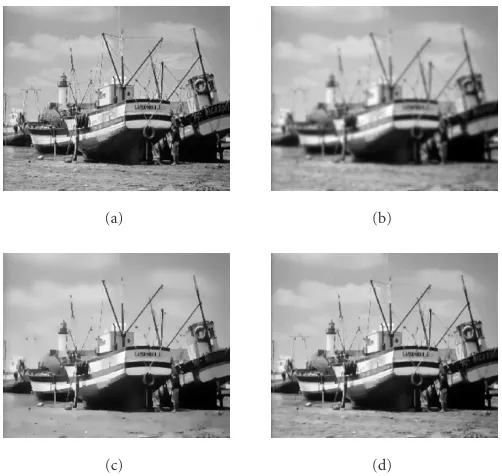
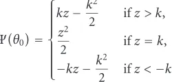
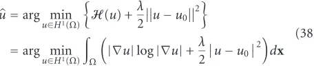
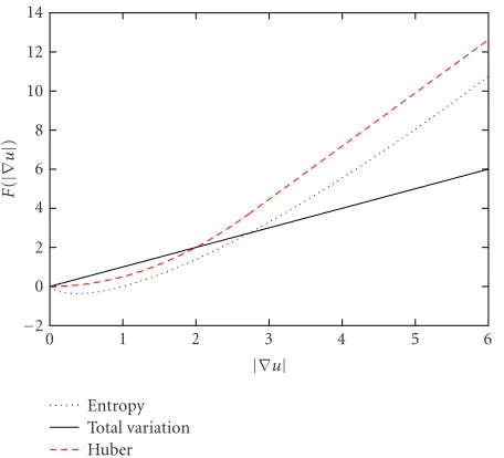
In order to evaluate the performance of the proposed gra-dient descent flows in the presence of Gaussian noise, the im-age shown inFigure 9ahas been corrupted by Gaussian white noise with SNR=4.79 dB.Figure 9displays the results of fil-tering the noisy image shown inFigure 9bby Huber with op-timalk=1.345, entropic, total variation, and improved en-tropic gradient descent flows. Qualitatively, we observe that the proposed techniques are able to suppress Gaussian noise while preserving important features in the image. The re-sulting MSE computations are depicted inTable 1.Figure 10
depicts another numerical example, and it clearly illustrates that the improved entropic flow performs the best. This fact is consistent with a variety of images used for experimenta-tion.
The Laplacian noise is somewhat heavier than the Gaus-sian noise. Moreover, the Laplace distribution is similar to Huber’s least favorable distribution [26] at least in the tails. To demonstrate the application of the proposed gradient descent flows to image denoising, qualitative and quantita-tive comparisons are performed to show a much improved performance of these techniques. Figure 11bshows a noisy image contaminated by Laplacian white noise with SNR =
(a) (b)
(c) (d)
(e) (f)
Figure9: Filtering results for Gaussian noise (Lena image): (a) original image, (b) noisy image, (c) Huber, (d) entropic, (e) total variation, and (f) improved entropic.
Table1: MSE’s computations for Gaussian noise.
PDE MSE
SNR=4.79 SNR=3.52 SNR=2.34
Huber 234.1499 233.7337 230.0263
Entropic 205.0146 207.1040 205.3454 Total variation 247.4875 263.0437 402.0660 Improved entropic 121.2550 137.9356 166.4490
The relative error versus the iteration number is illus-trated inFigure 12, where the convergence of the improved entropic flow is clearly demonstrated. The stopping criterion for the proposed flow isu(n+1)−u(n)2/u(n)
2 <, where is sufficiently small andndenotes thenth iteration.
8. DISCUSSIONS AND CONCLUSIONS
(a) (b)
(c) (d)
(e) (f)
Figure10: Filtering results for Gaussian noise (Cameraman image): (a) original image, (b) noisy image, (c) Huber, (d) entropic, (e) total variation, and (f) improved entropic.
by Gaussian as well as Laplacian noise, and it has been shown that these proposed techniques preserve details well while re-moving noise.
APPENDICES
A. DERIVATION OF GRADIENT FLOWS
The first variation of the functionalF(u)=ΩF(|∇u|)dxin the direction ofvis given by
δF(u;v)= d
dF(u+v)
=0
=
Ω
F|∇u|
|∇u| ∇u· ∇v
dx.
(A.1)
The identity
div(v∇u)=div(∇u)v+∇u· ∇v (A.2) yields
Ω
F|∇u|
|∇u| ∇u· ∇vdx = −
Ωdiv
F|∇u| |∇u| ∇u
v dx
+
Ωdiv
vF
|∇u|
|∇u| ∇u
dx.
(A.3)
Using the divergence theorem for a vector fieldw,
Ωdiv(w)dx=
(a) (b)
(c) (d)
(e) (f)
Figure11: Filtering results for Laplacian noise: (a) original image, (b) noisy image, (c) Huber, (d) entropic, (e) total variation, and (f) improved entropic.
Table2: MSE computations for Laplacian noise.
PDE MSE
SNR=6.33 SNR=3.91 SNR=3.05 Huber 237.7012 244.4348 248.4833 Entropic 200.5266 211.4027 217.3592 Total variation 138.4717 176.1719 213.1221 Improved entropic 104.4591 170.2140 208.8639
whereνis the outward unit normal vector (field) on∂Ω(the boundary ofΩ) anddsis an area element. Therefore,
Ωdiv
vF
|∇u| |∇u| ∇u
dx=
∂Ωv
F|∇u|
|∇u| ∇u·νds.
(A.5)
If we assume homogenuous Neumann boundary conditions
∇u·ν=uν =∂u∂ν =0, (A.6)
then the first variation ofF is reduced to
δF(u;v)= −
Ωdiv
F|∇u| |∇u| ∇u
vdx ∀v∈X (A.7)
which concludes the proof.
B. NUMERICAL IMPLEMENTATION OF GRADIENT FLOWS
50 100 150 200 250 300
Figure12: Improved entropic flow: relative error versus iteration number.
the matrices of column differences and row differences, re-spectively (i.e., backward and forward differences).
Similarly, the central differences are given by
Dx is discretized using an upwind scheme as follows:
divg|∇u|∇u
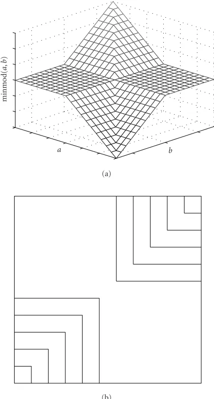
where minmod is a function that returns the argument with the smallest absolute value when all the arguments are of the same sign and zero otherwise. The minmod function is a lim-iter whose goal is to prevent oscillations while maintaining
a b
Figure 13: Illustration of minmod function: (a) 3D plot of the minmod function, (b) level curves.
the order of accuracy of the method, and it is defined as
minmod(a,b)=
ACKNOWLEDGMENTS
The authors would like to thank the anonymous review-ers for helpful and constructive comments. This work was in part supported by US Air Force Office of Scientific Re-search Grant no. F49620-98-1-0190, and by NATO Collabo-rative Linkage Grant no. 980107. Part of this work was con-ducted when H. Krim was visiting INRIA as an invited Pro-fessor.
REFERENCES
[1] D. Mumford and J. Shah, “Optimal approximations by piece-wise smooth functions and associated variational problems,” Comm. Pure Appl. Math., vol. 42, no. 5, pp. 577–685, 1989. [2] P. Perona and J. Malik, “Scale-space and edge detection using
anisotropic diffusion,” IEEE Trans. on Pattern Analysis and Machine Intelligence, vol. 12, no. 7, pp. 629–639, 1990. [3] L. Alvarez, P.-L. Lions, and J.-M. Morel, “Image selective
smoothing and edge detection by nonlinear diffusion. II,” SIAM J. Numer. Anal., vol. 29, no. 3, pp. 845–866, 1992. [4] L. Rudin, S. Osher, and E. Fatemi, “Nonlinear total variation
based noise removal algorithms,” Physica D, vol. 60, no. 1–4, pp. 259–268, 1992.
[5] L. Alvarez and L. Mazorra, “Signal and image restoration us-ing shock filters and anisotropic diffusion,” SIAM J. Numer. Anal., vol. 31, no. 2, pp. 590–605, 1994.
[6] J. Weickert,Anisotropic Diffusion in Image Processing, Teubner Verlag, Stuttgart, Germany, 1998.
[7] J.-M. Morel and S. Solimini, Variational Methods in Image Segmentation, Birkh¨auser, Boston, Mass, USA, 1995. [8] I. Pollak, A. S. Willsky, and H. Krim, “Image segmentation
and edge enhancement with stabilized inverse diffusion equa-tions,”IEEE Trans. Image Processing, vol. 9, no. 2, pp. 256–266, 2000.
[9] R. Deriche and O. Faugeras, “Les EDP en traitement des im-ages et vision par ordinateur,” Traitement du Signal, vol. 13, no. 6, pp. 59, 1996.
[10] P. Kornprobst, R. Deriche, and G. Aubert, “Image sequence analysis via partial differential equations,” J. Math. Imaging Vision, vol. 11, no. 1, pp. 5–26, 1999.
[11] C. Samson, L. Blanc-Feraud, G. Aubert, and J. Zerubia, “A variational model for image classification and restoration,” IEEE Trans. on Pattern Analysis and Machine Intelligence, vol. 22, no. 5, pp. 460–472, 2000.
[12] G. Aubert and L. Vese, “A variational method in image re-covery,”SIAM J. Numer. Anal., vol. 34, no. 5, pp. 1948–1979, 1997.
[13] H. Krim and I. C. Schick, “Minimax description length for signal denoising and optimized representation,” IEEE Trans-actions on Information Theory, vol. 45, no. 3, pp. 898–908, 1999.
[14] A. Ben Hamza and H. Krim, “Image denoising: a nonlinear robust statistical approach,”IEEE Trans. Signal Processing, vol. 49, no. 12, pp. 3045–3054, 2001.
[15] A. Yezzi, “Modified curvature motion for image smoothing and enhancement,” IEEE Trans. Image Processing, vol. 7, no. 3, pp. 345–352, 1998.
[16] P. Charbonnier, L. Blanc-Feraud, G. Aubert, and M. Barlaud, “Deterministic edge-preserving regularization in computed imaging,”IEEE Trans. Image Processing, vol. 6, no. 2, pp. 298– 311, 1997.
[17] M. Cetin and W. C. Karl, “Feature-enhanced synthetic aper-ture radar image formation based on nonquadratic regular-ization,”IEEE Trans. Image Processing, vol. 10, no. 4, pp. 623– 631, 2001.
[18] A. Ben Hamza and H. Krim, “A variational approach to max-imum a posteriori estimation for image denoising,” inEnergy Minimization Methods in Computer Vision and Pattern Recog-nition, vol. 2134 of Lecture Notes in Computer Science, pp. 19–34, Springer-Verlag, New York, NY, USA, 2001.
[19] T. F. Chan and C.-K. Wong, “Total variation blind deconvolu-tion,”IEEE Trans. Image Processing, vol. 7, no. 3, pp. 370–375, 1998.
[20] T. F. Chan, S. Osher, and J. Shen, “The digital TV filter and nonlinear denoising,” IEEE Trans. Image Processing, vol. 10, no. 2, pp. 231–241, 2001.
[21] M. Giaquinta and S. Hildebrandt, Calculus of Variations I: The Lagrangian Formalism, Springer-Verlag, Berlin, Germany, 1996.
[22] T. F. Chan and P. Mulet, “On the convergence of the lagged diffusivity fixed point method in total variation image restora-tion,”SIAM J. Numer. Anal., vol. 36, no. 2, pp. 354–367, 1999. [23] K. Ito and K. Kunisch, “Restoration of edge-flat-grey scale images,”Inverse Problems, vol. 16, no. 4, pp. 909–928, 2000. [24] S. Geman and D. Geman, “Stochastic relaxation, Gibbs
distri-butions, and the Bayesian restoration of images,”IEEE Trans. on Pattern Analysis and Machine Intelligence, vol. 6, no. 6, pp. 721–741, 1984.
[25] Y.-L. You, W. Xu, A. Tannenbaum, and M. Kaveh, “Behavioral analysis of anisotropic diffusion in image processing,” IEEE Trans. Image Processing, vol. 5, no. 11, pp. 1539–1553, 1996. [26] P. Huber,Robust Statistics, John Wiley & Sons, New York, NY,
USA, 1981.
[27] M. J. Black, G. Sapiro, D. H. Marimont, and D. Heeger, “Ro-bust anisotropic diffusion,”IEEE Trans. Image Processing, vol. 7, no. 3, pp. 421–432, 1998.
[28] A. Ben Hamza and H. Krim, “Robust influence functionals for image filtering,” inProc. IEEE International Conference on Image Processing (ICIP ’03), vol. 3, pp. 361–364, Barcelona, Spain, September 2003.
[29] G. Gallager,Information Theory and Reliable Communication, John Wiley & Sons, New York, NY, USA, 1968.
[30] H. Krim, “On the distributions of optimized multiscale rep-resentations,” inProc. IEEE Int. Conf. Acoustics, Speech, Signal Processing (ICASSP ’97), vol. 5, pp. 3673–3676, Munich, Ger-many, April 1997.
A. Ben Hamza received his Ph.D. degree in electrical engineering from North Car-olina State University in 2003, where he worked on variational methods in imag-ing and computer vision, and information theory. Prior to joining Concordia Insti-tute for Information Systems Engineering, Concordia University, he was a Postdoc-toral Associate at Duke University, affi li-ated with both the Department of
Hamid Krim received his B.S., M.S., and Ph.D. degrees in electrical engineering from the University of Southern California, the University of Washington, and Northeast-ern University, respectively. As a member of the technical staff at AT&T Bell Labs, he worked in the area of telephony and digital communication systems/subsystems. In 1991, he became a US National Science Foundation Postdoctoral Scholar at the
For-eign Centers of Excellence (LSS Supelec/University of Orsay, Paris, France). He subsequently joined the Laboratory for Informa-tion and Decision Systems, Massachusetts Institute of Technol-ogy, Cambridge, Massachusetts, as a Research Scientist perform-ing/supervising research in his area of interest, and later became a faculty member in the Electrical and Computer Engineering De-partment, North Carolina State University in Raleigh in 1998. He is an original contributor and now an Affiliate of the Center for Imaging Science sponsored by the US Army. He is also a recipient of the US National Science Foundation Career Young Investigator Award. He is a Senior Member of the IEEE and a Member of the IEEE Computer Society.
Josiane Zerubiahas been a Permanent Re-search Scientist at INRIA since 1989. She has been the Director of Research since July 1995. Since January 1998, she has been in charge of a research group working on re-mote sensing (ARIANA). She has been an Adjunct Professor at Sup’Aero (ENSAE) in Toulouse since 1999. Before, she was at the University of Southern California in Los Angeles as a Postdoc. She also worked as a