Volume 2007, Article ID 14798,10pages doi:10.1155/2007/14798
Research Article
Capacity Versus Bit Error Rate Trade-Off in
the DVB-S2 Forward Link
Matteo Berioli, Christian Kissling, and R ´emi Lapeyre
German Aerospace Center (DLR), Institute of Communications and Navigation, Oberpfaffenhofen, 82234 Wessling, Germany
Received 5 October 2006; Accepted 12 March 2007
Recommended by Ray E. Sheriff
The paper presents an approach to optimize the use of satellite capacity in DVB-S2 forward links. By reducing the so-called safety margins, in the adaptive coding and modulation technique, it is possible to increase the spectral efficiency at expenses of an increased BER on the transmission. The work shows how a system can be tuned to operate at different degrees of this trade-off, and also the performance which can be achieved in terms of BER/PER, spectral efficiency, and interarrival, duration, strength of the error bursts. The paper also describes how a Markov chain can be used to model the ModCod transitions in a DVB-S2 system, and it presents results for the calculation of the transition probabilities in two cases.
Copyright © 2007 Matteo Berioli et al. This is an open access article distributed under the Creative Commons Attribution License, which permits unrestricted use, distribution, and reproduction in any medium, provided the original work is properly cited.
1. INTRODUCTION
The original DVB-S standard dates back to 1995 and was in-tended for delivery of broadcasting services, the underlying transport stream of S was defined to be MPEG-2. DVB-S2 [1] is the second generation of the DVB-S standard and comprises a variety of new features. It can be used for provi-sion of HDTV (high definition televiprovi-sion) but it also allows for transportation of different multimedia streams such as, for example, internet traffic, audio and video streaming and file transfers with support of different input stream formats such as IP, ATM, single/multiple MPEG streams or generic bit streams, both for broadcast and unicast transmissions. For the support of interactive applications a return channel is necessary which can be provided by RCS [2]. DVB-S2 can achieve a capacity increase of up to 30% under the same transmission conditions compared to the older DVB-S standard what is achieved by applying higher order modu-lation schemes and by the use of low density parity check codes (LDPC) and Bose-Chaudhuri-Hochquenghem (BCH) codes.
The real novelty introduced by DVB-S2 was the pos-sibility to use adaptive coding and modulation (ACM). In traditional nonadaptive systems the link dimensioning has to be made under considerations of service availability and worst case channel assumptions due to the deep fades caused by atmospheric effects; as a consequence the classical fade
mitigation techniques like power control result in an inef-ficient use of the system capacity since most of the time more transponder power than necessary is used. On the other hand in case of ACM, if a terminal is able to inform the gateway of its particular channel conditions (by means of a proper re-turn link) the gateway can select an appropriate waveform, coding and modulation, to best exploit the spectrum and at the same time to overcome the channel impairments.
An efficient exploitation of the expensive satellite capac-ity has always been a key factor in the development of the satellite market, and the improvements brought by DVB-S2 give promising perspectives for the future of satellite commu-nications. Nevertheless it is important to keep improving the exploitation of the satellite bandwidth, in order to guaran-tee reduced costs for all satellite services (broadcast, Internet, etc.). The aim of this work is to go one step further in this trend and to try to optimize the throughput and the spec-trum efficiency in DVB-S2 forward links.
Today DVB-S2 links offer to the higher-layers protocols a terrestrial-like transmission medium, with recommended PERs around 10−7. This is of course an excellent result, but not all services at higher layers require to reach such out-standing performance. This is in particular true for Internet and multimedia services [3].
Other modern media codecs (e.g., MPEG-4 [5]) have been designed to be highly resilient to residual errors in the in-put bit-stream, to detect and localize errors within the packet payload, and to employ concealment techniques, like for in-stance interframe interpolation, that hide errors from a hu-man user. These codecs offer acceptable quality at a resid-ual BER poorer than 10−3, and some at poorer than 10−2 [6]. In order to support these error-tolerant codecs, the IETF has also standardized a new multimedia transport proto-col, UDP-Lite [7], that allows to specify the required level of payload protection, while maintaining end-to-end delivery checks (verification of intended destination, IP header fields and overall length).
When these services are operating over the satellite con-nection, it is convenient to reduce the quality of the trans-mission in DVB-S2 forward links, by allowing higher BERs, in order to increase the precious capacity and the through-put. The first motivation for this is to make use of cross-layer mechanisms by voluntarily allowing higher bit error rates which can be compensated with error correction at higher layers. A second motivation to allow for higher BERs is that not all applications have the same stringent BER require-ments. This represents a natural trade-offbetween errors and capacity. The present work analyzes this trade-off, proposes a way to tune the system parameters in order to work in optimal conditions, and investigates the performance of the system in this situation. The work is organized as follows: Section 2presents the background and the scenario of the subject,Section 3describes the main ideas of the paper and the original approach to the problem,Section 4evaluates the performance of a system operating in the suggested condi-tions, andSection 5drives the conclusions of the paper.
2. BACKGROUND AND SCENARIO
2.1. Overview of DVB-S2
The second generation of DVB-S provides a new way of fade mitigation by means of adaptation of the coding and modu-lation (ACM) to the different channel states. This of course implies the need for every terminal to signal its perceived channel state back to the gateway which can then make a frame-by-frame decision of the modulation and coding com-bination (ModCod) to be applied based on these measure-ments. DVB-S2 offers a broad range of modulations and cod-ings for ACM. The supported modulation schemes comprise QPSK, 8-PSK, 16-APSK, 32-APSK and considered coding rates are 1/4, 3/4, 1/3, 2/5, 3/5, 4/5, 1/2, 5/6, 8/9, 9/10. The possibility to select the modulation and coding for an indi-vidual destination allows to make a more efficient use of the system capacity since transmission in a higher-order modu-lation in combination with a low coding rate (e.g., for clear sky conditions) allows to transmit more bits per symbol than a low-order modulation with high coding rate (e.g., for rainy channels). In this way it is possible to use individually for ev-ery ground terminal (or for evev-ery group of terminals in the same spot beam) the highest possible modulation scheme and the lowest coding rate which still allows to cope with
the channel impairments to provide low BER. A destination with a bad channel state can thus use a very robust modula-tion and coding pair (ModCod) while other terminals with a very good channel state can still transmit in highly efficient ModCods. The adaptive selection of the best suited ModCod results in an increased net data throughput while terminals in bad channel conditions are still able to receive their data since they can use ModCods with lower-order modulation and higher coding (but at the cost of lower spectral efficiency and thus lower throughput).
As can be seen in Figure 1 the system architecture of DVB-S2 is subdivided into six main components [1]. The mode adaptation subsystem provides an interface to the ap-plication specific data stream formats and also contains a CRC-8 error detection coding scheme. It is possible to merge different input streams together and to segment them into the called data fields which are the payload part of the so-called baseband-frames (BBFRAME) created at the output of the consecutive stream adaptation module. Buffers store data until they are processed by the merger/slicer and in case not enough data is available to fill a data field or if it is re-quired to have only an integer number of packets in a frame (in general integer number of packets will not perfectly fit into a frame but their payload sum will always be slightly smaller or larger than the data field), the unused space can be padded, this operation is accomplished by the stream adap-tation subsystem. In order to complete the baseband frame (BBFRAME) additional header information (BBHEADER) is added in front of the data field and scrambling of header and payload is applied. The final BBFRAME structure is il-lustrated inFigure 2.
Single
Figure1: DVB-S2 system architecture [1].
80 bits DFL Kbch-DFL-80
BBHEADER Data field Padding
BBFRAME (Kbchbits)
Figure2: Structure of a BBFRAME [1].
Nbch=kldpc
Kbch Nbch-Kbch nldpc-kldpc
BBFRAME BCHFEC LDPCFEC
(nldpcbits)
Figure3: Structure of a FECFRAME [1].
For the selection of a ModCod that is adapting to the in-dividual experienced channel states of the terminals, a return link must be provided to give feedback information about the measured channel states to the gateway. The gateway can then use this information to select a ModCod that suits trans-missions in this channel state. This means the ModCod is selected to provide a quasi-error-free transmission as long as the critical SNR (signal-to-noise ratio) demodulation thresh-old for this ModCod (thrdem(ModCod)) is not crossed. If the signal drops below thrdem(ModCod) then the BER will dras-tically increase due to the nature of the applied LDPC and BCH coding of having very steep BER-versus-SNR curves. In the GEO-stationary scenario investigated here, the propaga-tion delay of the informapropaga-tion feedback from the terminal to the gateway takes relatively long and it is in the order of
sev-eral hundreds milliseconds (250 milliseconds). This means that though the order of magnitude for the propagation de-lay allows for a compensation of very slow changing channel effects, like rain attenuation, it is too long to compensate fast, high-frequent changes in the SNR as those caused by scintil-lation, this will be explained in the next section.
2.2. Channel modelling
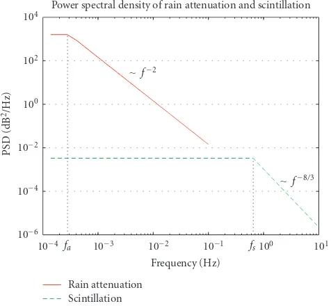
The selection of a ModCod scheme for transmission is very decisive for the performance of the system in terms of net data rate, bit errors and, respectively, packet errors. If the ModCods are selected too aggressively (meaning selection of ModCods with a too high modulation scheme and a too low coding) the transmission will result in a drastically higher PER. On the other hand, selection of safe ModCods (mean-ing a ModCod with a modulation lower than what would be necessary and a coding higher than necessary) will result in inefficiencies which reflects in a lower net data rate. In or-der to evaluate the influence of different parameters for the ModCod selection it is important to have a realistic chan-nel model. The chanchan-nels in satellite systems face mainly two sources of signal fading, rain attenuation and scintillation. The effect of rain attenuation is very significant for systems operating in K-band where the signal is attenuated by ab-sorbing effects of the water. The second effect coming along with rain attenuation is scintillation which is basically a high frequent distortion of the signal amplitude and phase caused by small-scale irregularities in electron density in the iono-sphere [8].
101
Power spectral density of rain attenuation and scintillation
Rain attenuation Scintillation
∼f−8/3
∼f−2
Figure4: Attenuation and scintillation spectrum (typical values:
fa≈10−4Hz,fs≈0.1−0.65 Hz).
of the scintillation process can be calculated according to (1) corresponding to the theory of Tatarskii [9] and the model of Matricciani [10],
σ=σ0·A5/12. (1)
The valueσ0is the standard deviation of the scintillation for a rain attenuation ofA[dB]. [10] suggests a typical value of 0.039 forσ0in the frequency range of 19.77 GHz. According to (1) the resulting scintillation standard deviationσis then in the order of tenths of a dB for rain attenuations smaller than 20 dB.
Within this work the main focus is on the scintillation effects since these cannot be compensated by signalling of the channel states via the return channel because of the long propagation delay of the GEO satellite. Nevertheless the channel simulations used in the rest of this work consider spatial correlated rain attenuation as well since the magni-tude of the scintillation also depends on the intensity of the rain attenuation (see (1)). Similar to the generation of the scintillation, also the rain attenuation is created via a normal distributed random variable whereas its spectrum has a dif-ferent corner frequency of fa(see alsoFigure 4).
Figure 5 shows a channel example for the attenuation caused by scintillation and rain for a user located at longi-tude 8.6◦E and latitude 52.7◦N, in the area around Hamburg (Germany). It can be seen here that scintillation effects occur with a much higher frequency than regular rain attenuation events and how rain attenuation and scintillation are corre-lated.
2.3. ModCod switching strategies
While the rain attenuation occurs on a larger time scale scin-tillation effects occur very rapidly. For this reason rain
fad-8000
Figure5: Example of scintillation and rain attenuation.
ing can be mitigated by mode adaptation whereas counter-measures for scintillation require a different compensation. For every combination of modulation and coding a threshold thrdem(ModCod) exists which is needed to be able to decode the frame with a quasi-zero BER. The decision of the gateway on which ModCod will be used is thus driven by thresholds. For switching among ModCods these thresholds could theo-retically be used directly for the decision about which Mod-Cod will be used, but in practice this would result in frequent transmission errors since the high frequent variations of the channel (due to scintillation) would cause a frequent crossing of the threshold. On the one hand, this high frequent cross-ing cannot be compensated by signallcross-ing to the gateway, on the other hand such signalling would also mean a high fre-quent change of the ModCod which is as well undesirable.
To provide more reliability the minimal needed demod-ulation thresholds thrdem (ModCod) can be replaced by thresholds which have a certain safety margin. This means that a lower ModCod is selected already before the critical threshold (the threshold below which a strong increase in bit error rate occurs) is reached. The size of the safety mar-gin does thus determine the robustness against fast occurring scintillation fades. On the other hand, this size of the safety margin also influences the system performance since trans-mission in a higher ModCod would result in a higher net data rate. Since fast oscillations between neighboring Mod-Cods are also possible when safety margins are used, an ad-ditional hysteresis margin is introduced.Figure 6illustrates the different thresholds and margins.
WithinFigure 6the terms thrdem(N−1) and thrdem(N) denote the minimum SNR values which are just enough to provide quasi error free decoding. If, for example, ModCod
ModCod (thrdem(N) in this case) is crossed but after a higher threshold is exceeded (threnable(N−1)).
In case the signal strength decreases again, the ModCod is not switched when the enabling threshold threnableis crossed, but just when an additional hysteresis margin is exceeded. The threshold for switching to a smaller ModCod is denoted as thrdown(ModCod) and the size of the hysteresis margin as (Δthrhyst(N)). The distance between the critical demodula-tion threshold thrdem(ModCod) and the threshold that trig-gers a downswitching thrdown(ModCod) is called the safety marginΔthrsafety(ModCod).
The safety margin(Δthrsafety(ModCod)) can be seen as an additional security for high frequent oscillations which cannot be countervailed due to the long satellite propagation delay. If the signal strength oscillates within this area no in-crease in BER will occur since the thrdem(ModCod) thresh-old is not crossed. The values for the safety margin and the hysteresis margin can be varied and they can also be different for every ModCod. W¨orz et al. [11] presented a calculation method for all aforementioned parameters which provides a quasi error free system performance. The calculation of the parameters in [11] mainly depends on estimated values of the scintillation standard deviations and a numerically de-rived function which accounts for the fact that the standard deviation of the scintillation is also dependent on the inten-sity of the rain attenuation.
Within the remaining parts of this work the influence of the size of the safety margins with respect to gain or loss in channel net efficiency and increase/decrease of BER is inves-tigated. The term “W¨orz-Schweikert safety margins” denotes the safety margins calculated according to the algorithm pre-sented in [11] while “zero-safety margin” denotes the fact that no safety margin is used.
2.4. Investigated environment
Within the examined scenarios, a set of user terminals has been located in a geographical region close to the city of Hamburg, Germany (longitude 9.5◦−10.5◦E, latitude 52.5◦− 54◦N) within the aforementioned channel simulator. The set comprises 38 different terminal locations whereby the chan-nel states are sampled with 10 Hz. The investigated duration is 7200 seconds per simulation run. In order to get statistical significant results the simulation duration of 7200 seconds per simulation have been extended to 60 hours. The 60 hours channel simulation results for the 38 terminals can be seen as 2280 hours of simulated channel states for a single terminal what in turn means that all results are based on channel in-formation which corresponds to roughly a quarter of a year.
3. SYSTEM MODELLING
The main idea behind this study is that by reducing the safety margin in the ModCod switching strategy it is possible to gain in spectral efficiency, and thus to increase the net data throughput, at the expenses of an increased BER (and con-sequently a higher PER). In order to investigate this and to derive a detailed quantitative estimation of this trade-off, it
ModCodN−1 ModCodN
threnable(N−1)
thrdown(N−1)
Δthrsafety(N−1)
thrdem(N−1)
Δthrhyst(N)
Δthrsafety(N)
No switching here because of hysteresis
Signal
thrdown(N)
thrdem(N)
Time
SNIR
Figure6: Illustration on the different thresholds.
is important to carefully describe the assumptions on which the analysis is based, this is what is presented in this sec-tion. Though the obtained results have a quantitative mean-ing only considermean-ing these assumptions, it is worth statmean-ing that their qualitative relevance has a general importance, as it will be later explained.
Existing systems compliant with the DVB-S2 standard can provide the higher-layers protocols with a quasi-error-free underlaying physical layer (PER =10−7). For this pur-pose regular 8-bytes CRC (cyclic redundancy check) fields are used to identify errors in the BBFRAME, which were not corrected by the coding schemes (LDPC and BCH) at re-ception. In case an error is detected in a frame, it has to be considered that the wrong bit(s) cannot be singularly identi-fied in the frame, so one of the two following choices can be made:
(1) the whole frame is discarded (this is what is normally done);
(2) the packets in the frame are passed to the higher proto-cols with uncorrected failures (this can be done in case the higher protocols are able to cope with errors).
These cases are very rare when high safety margins are adopted, and systems are normally dimensioned to avoid them, but they become more frequent if the system works closer to the demodulation thresholds (as we defined them in the previous section), for the reasons already explained.
If a system is dimensioned also to operate in these con-ditions, it is important to evaluate the statistical properties and characteristics of these situations, that is, how often they occur and what failures they bring in comparison to the ca-pacity gain. In order to do that we performed three levels of analysis. They are theoretically described in this sections, whereas the results obtained for each of them are shown and discussed in the next one.
3.1. Markov model
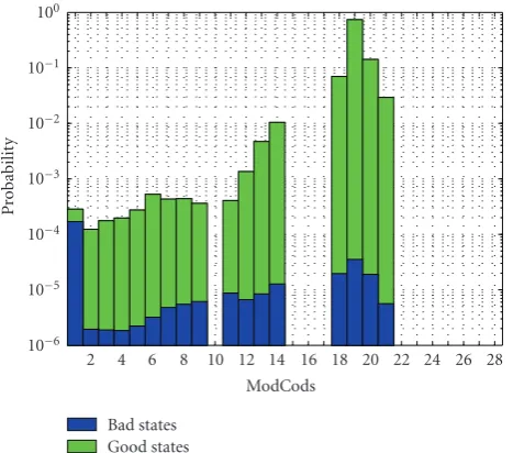
The best way to show the difference between the two ap-proaches is to model the system according to a Markov chain, where each state represents the system operating with one particular ModCod. The chain presents two states for each ModCodN: the good one,NG, and the bad one,NB; so the overall number of states is twice the total amount of allowed ModCods (56). In the good state the SNR measured at the re-ceiver is above the demodulating threshold for that ModCod, and so no failures are expected, in the bad state the system SNR is below the demodulating threshold for that ModCod, and so failures may occur with probabilities that are not neg-ligible.
A similar Markov chain is an excellent model, because it summarizes very well the properties of a ModCod switch-ing approach. So once the transition probabilities for one particular ModCod switching criterion have been calculated (normally by simulations), the Markov chain can be used as a basis for all types of analysis without the need of run-ning again computationally heavy simulations, which might be very long in order to gather statistically meaningful data. In this sense the calculated Markov chain (i.e., the ModCod transition probabilities) can be considered independent from the simulated channel conditions, only if the simulation is long enough to represent general channel statistics. On the other hand, it should be mentioned that the same Markov chain depends on some parameters which might be charac-teristic of particular cases, for example, the link budget in clear sky, and consequently the system availability. So even if the resulting numbers are only meaningful bearing in mind these assumptions, the quantitative conclusions which can be derived have general relevance, and this will be clearer in the next section.
3.2. Error rate versus capacity trade-off
The second level of analysis describes the details of each state of the Markov chain. The good states present quasi-error-free conditions according to the DVB-S2 recommendations, so PER = 10−7. Since the BER versus SNR characteristics for all ModCods are very steep, the BER values increase quite rapidly when the SNR level goes below the demodulating threshold. In particular they change of several orders of mag-nitude within a few tenths of dB, going from BER≈ 10−10 when SNR is close or bigger than the demodulating thresh-olds, up to BER ≈ 10−2 when the SNR is just 0.3 dB be-low the threshold. Each bad state represents a set of different BERs, the proper BER is selected at each time step according to the received level of SNR with respect to the demodulat-ing thresholds. The exact characteristics for the BER-versus-SNR functions, which were used in the simulations and to derive the Markov chain parameters, were taken from [12]. In that work, end-to-end performances of the BER versus the SNR are presented for the DVB-S2 system, the whole communication chain is modelled and simulated, including coding, modulation with predistortion techniques, satellite transponder impairments, downlink, demodulation with the synchronization, and the final LDPC and BCH decoders. In the Markov chain, each ModCod might have its own BER
versus SNR characteristic, but to use one single function for all ModCods already seems an excellent approximation to the real case, so this is how it was implemented in the simulator. PERs are derived from these BERs under consideration of the payload length of each BBFRAME also regarding the applied ModCod. A BBFRAME is considered as erroneous if at least one of the payload bits is erroneous. For the rest of this paper the term PER denotes the BBFRAME packet error rate. Thanks to this definition of the states of Markov chain, this model allows to derive the properties of the communi-cation in terms of PER and BER statistics, and by knowing the spectral efficiency associated to each ModCod it is easy to derive an average resulting capacity.
3.3. Error bursts analysis
The third and last level of analysis goes into the details of the failures introduced with this novel approach. In the previous section we explained how to derive a measure of the trade-offbetween average capacity and average BER (or PER). An average measure of the BER (or PER) does not seem a very precise information, since these failures come in bursts. The errors are mainly due to the ModCod switchings, and they are mostly introduced by reduced safety margins. So we want to investigate three main properties: (i) how often the error bursts arrive (interarrival times statistics), (ii) how long the bursts last (duration statistics), and (iii) how deep the fades are (i.e., how high are BER and PER during one error burst). These three properties can be estimated thanks to the Markov model, and this analysis produces interesting information, which will be presented in the next section.
4. RESULTS EVALUATION
4.1. Markov model
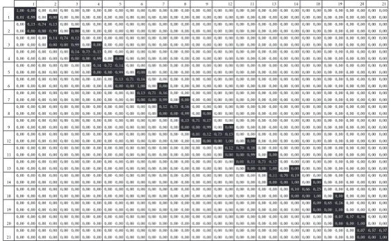
A software simulator was developed in order to derive the Markov model presented in the previous section. Once the ModCod switching criterion has been specified the software simulates the evolution over time of the system; from these simulations we can derive statistics about the permanence in the different ModCods for each ModCod switching criterion, this was done by computing transition matrices and solving them. In the following we present two full transition matrices for two different ModCod switching criteria.
Simulations equivalent to 3 months of SNR time series have been carried out, one using W¨orz-Schweikert safety margins, the other one using zero-safety margin bounds with W¨orz-Schweikert hysteresis bounds.
1 2 3 4 5 6 7 8 9
1, 00 0, 000, 00 0, 00 0, 00 0, 00 0, 00 0, 00 0, 00 0, 00 0, 00 0, 00 0, 00 0, 00 0, 00 0, 00 0, 00 0, 00 0, 00 0, 00 0, 00 0, 00 0, 00 0, 00 0, 00 0, 00 0, 00 0, 00 0, 00 0, 00 0, 00 0, 00 0, 00 0, 00 1 0, 01 0, 990, 000, 000, 00 0, 00 0, 00 0, 00 0, 00 0, 00 0, 00 0, 00 0, 00 0, 00 0, 00 0, 00 0, 00 0, 00 0, 00 0, 00 0, 00 0, 00 0, 00 0, 00 0, 00 0, 00 0, 00 0, 00 0, 00 0, 00 0, 00 0, 00 0, 00 0, 00 0, 000, 13 0, 74 0, 130, 00 0, 00 0, 00 0, 00 0, 00 0, 00 0, 00 0, 00 0, 00 0, 00 0, 00 0, 00 0, 00 0, 00 0, 00 0, 00 0, 00 0, 00 0, 00 0, 00 0, 00 0, 00 0, 00 0, 00 0, 00 0, 00 0, 00 0, 00 0, 00 0, 00 2 0, 000, 00 0, 00 0, 990, 000, 000, 00 0, 00 0, 00 0, 00 0, 00 0, 00 0, 00 0, 00 0, 00 0, 00 0, 00 0, 00 0, 00 0, 00 0, 00 0, 00 0, 00 0, 00 0, 00 0, 00 0, 00 0, 00 0, 00 0, 00 0, 00 0, 00 0, 00 0, 00 0, 00 0, 00 0, 000, 14 0, 74 0, 120, 00 0, 00 0, 00 0, 00 0, 00 0, 00 0, 00 0, 00 0, 00 0, 00 0, 00 0, 00 0, 00 0, 00 0, 00 0, 00 0, 00 0, 00 0, 00 0, 00 0, 00 0, 00 0, 00 0, 00 0, 00 0, 00 0, 00 0, 00 3 0, 00 0, 00 0, 000, 00 0, 00 0, 990, 000, 000, 00 0, 00 0, 00 0, 00 0, 00 0, 00 0, 00 0, 00 0, 00 0, 00 0, 00 0, 00 0, 00 0, 00 0, 00 0, 00 0, 00 0, 00 0, 00 0, 00 0, 00 0, 00 0, 00 0, 00 0, 00 0, 00 0, 00 0, 00 0, 00 0, 00 0, 000, 14 0, 73 0, 130, 00 0, 00 0, 00 0, 00 0, 00 0, 00 0, 00 0, 00 0, 00 0, 00 0, 00 0, 00 0, 00 0, 00 0, 00 0, 00 0, 00 0, 00 0, 00 0, 00 0, 00 0, 00 0, 00 0, 00 0, 00 0, 00 4 0, 00 0, 00 0, 00 0, 00 0, 000, 00 0, 00 0, 990, 000, 000, 00 0, 00 0, 00 0, 00 0, 00 0, 00 0, 00 0, 00 0, 00 0, 00 0, 00 0, 00 0, 00 0, 00 0, 00 0, 00 0, 00 0, 00 0, 00 0, 00 0, 00 0, 00 0, 00 0, 00 0, 00 0, 00 0, 00 0, 00 0, 00 0, 00 0, 000, 14 0, 72 0, 140, 00 0, 00 0, 00 0, 00 0, 00 0, 00 0, 00 0, 00 0, 00 0, 00 0, 00 0, 00 0, 00 0, 00 0, 00 0, 00 0, 00 0, 00 0, 00 0, 00 0, 00 0, 00 0, 00 0, 00 5 0, 00 0, 00 0, 00 0, 00 0, 00 0, 00 0, 000, 00 0, 00 0, 990, 000, 000, 00 0, 00 0, 00 0, 00 0, 00 0, 00 0, 00 0, 00 0, 00 0, 00 0, 00 0, 00 0, 00 0, 00 0, 00 0, 00 0, 00 0, 00 0, 00 0, 00 0, 00 0, 00 0, 00 0, 00 0, 00 0, 00 0, 00 0, 00 0, 00 0, 00 0, 000, 13 0, 71 0, 160, 00 0, 00 0, 00 0, 00 0, 00 0, 00 0, 00 0, 00 0, 00 0, 00 0, 00 0, 00 0, 00 0, 00 0, 00 0, 00 0, 00 0, 00 0, 00 0, 00 0, 00 0, 00 6 0, 00 0, 00 0, 00 0, 00 0, 00 0, 00 0, 00 0, 00 0, 000, 00 0, 00 1, 000, 000, 000, 00 0, 00 0, 00 0, 00 0, 00 0, 00 0, 00 0, 00 0, 00 0, 00 0, 00 0, 00 0, 00 0, 00 0, 00 0, 00 0, 00 0, 00 0, 00 0, 00 0, 00 0, 00 0, 00 0, 00 0, 00 0, 00 0, 00 0, 00 0, 00 0, 00 0, 000, 13 0, 71 0, 160, 00 0, 00 0, 00 0, 00 0, 00 0, 00 0, 00 0, 00 0, 00 0, 00 0, 00 0, 00 0, 00 0, 00 0, 00 0, 00 0, 00 0, 00 0, 00 0, 00 7 0, 00 0, 00 0, 00 0, 00 0, 00 0, 00 0, 00 0, 00 0, 00 0, 00 0, 000, 00 0, 00 0, 990, 000, 000, 00 0, 00 0, 00 0, 00 0, 00 0, 00 0, 00 0, 00 0, 00 0, 00 0, 00 0, 00 0, 00 0, 00 0, 00 0, 00 0, 00 0, 00 0, 00 0, 00 0, 00 0, 00 0, 00 0, 00 0, 00 0, 00 0, 00 0, 00 0, 00 0, 00 0, 000, 12 0, 71 0, 160, 00 0, 00 0, 00 0, 00 0, 00 0, 00 0, 00 0, 00 0, 00 0, 00 0, 00 0, 00 0, 00 0, 00 0, 00 0, 00 0, 00 0, 00 8 0, 00 0, 00 0, 00 0, 00 0, 00 0, 00 0, 00 0, 00 0, 00 0, 00 0, 00 0, 00 0, 000, 00 0, 00 0, 990, 000, 000, 00 0, 00 0, 00 0, 00 0, 00 0, 00 0, 00 0, 00 0, 00 0, 00 0, 00 0, 00 0, 00 0, 00 0, 00 0, 00 0, 00 0, 00 0, 00 0, 00 0, 00 0, 00 0, 00 0, 00 0, 00 0, 00 0, 00 0, 00 0, 00 0, 00 0, 000, 13 0, 71 0, 170, 00 0, 00 0, 00 0, 00 0, 00 0, 00 0, 00 0, 00 0, 00 0, 00 0, 00 0, 00 0, 00 0, 00 0, 00 0, 00 9 0, 00 0, 00 0, 00 0, 00 0, 00 0, 00 0, 00 0, 00 0, 00 0, 00 0, 00 0, 00 0, 00 0, 00 0, 000, 00 0, 00 0, 990, 000, 000, 00 0, 00 0, 00 0, 00 0, 00 0, 00 0, 00 0, 00 0, 00 0, 00 0, 00 0, 00 0, 00 0, 00 0, 00 0, 00 0, 00 0, 00 0, 00 0, 00 0, 00 0, 00 0, 00 0, 00 0, 00 0, 00 0, 00 0, 00 0, 00 0, 000, 01 0, 12 0, 73 0, 150, 00 0, 00 0, 00 0, 00 0, 00 0, 00 0, 00 0, 00 0, 00 0, 00 0, 00 0, 00 0, 00 0, 00 12 0, 00 0, 00 0, 00 0, 00 0, 00 0, 00 0, 00 0, 00 0, 00 0, 00 0, 00 0, 00 0, 00 0, 00 0, 00 0, 00 0, 000, 00 0, 00 1, 000, 000, 000, 00 0, 00 0, 00 0, 00 0, 00 0, 00 0, 00 0, 00 0, 00 0, 00 0, 00 0, 00 0, 00 0, 00 0, 00 0, 00 0, 00 0, 00 0, 00 0, 00 0, 00 0, 00 0, 00 0, 00 0, 00 0, 00 0, 00 0, 00 0, 00 0, 00 0, 000, 12 0, 70 0, 180, 00 0, 00 0, 00 0, 00 0, 00 0, 00 0, 00 0, 00 0, 00 0, 00 0, 00 0, 00 11 0, 00 0, 00 0, 00 0, 00 0, 00 0, 00 0, 00 0, 00 0, 00 0, 00 0, 00 0, 00 0, 00 0, 00 0, 00 0, 00 0, 00 0, 00 0, 000, 00 0, 00 0, 990, 000, 000, 00 0, 00 0, 00 0, 00 0, 00 0, 00 0, 00 0, 00 0, 00 0, 00 0, 00 0, 00 0, 00 0, 00 0, 00 0, 00 0, 00 0, 00 0, 00 0, 00 0, 00 0, 00 0, 00 0, 00 0, 00 0, 00 0, 00 0, 00 0, 00 0, 000, 01 0, 11 0, 71 0, 170, 00 0, 00 0, 00 0, 00 0, 00 0, 00 0, 00 0, 00 0, 00 0, 00 13 0, 00 0, 00 0, 00 0, 00 0, 00 0, 00 0, 00 0, 00 0, 00 0, 00 0, 00 0, 00 0, 00 0, 00 0, 00 0, 00 0, 00 0, 00 0, 00 0, 00 0, 000, 00 0, 00 1, 000, 000, 000, 00 0, 00 0, 00 0, 00 0, 00 0, 00 0, 00 0, 00 0, 00 0, 00 0, 00 0, 00 0, 00 0, 00 0, 00 0, 00 0, 00 0, 00 0, 00 0, 00 0, 00 0, 00 0, 00 0, 00 0, 00 0, 00 0, 00 0, 00 0, 00 0, 00 0, 000, 11 0, 70 0, 190, 00 0, 00 0, 00 0, 00 0, 00 0, 00 0, 00 0, 00 14 0, 00 0, 00 0, 00 0, 00 0, 00 0, 00 0, 00 0, 00 0, 00 0, 00 0, 00 0, 00 0, 00 0, 00 0, 00 0, 00 0, 00 0, 00 0, 00 0, 00 0, 00 0, 00 0, 000, 00 0, 00 1, 000, 000, 000, 00 0, 00 0, 00 0, 00 0, 00 0, 00 0, 00 0, 00 0, 00 0, 00 0, 00 0, 00 0, 00 0, 00 0, 00 0, 00 0, 00 0, 00 0, 00 0, 00 0, 00 0, 00 0, 00 0, 00 0, 00 0, 00 0, 00 0, 00 0, 00 0, 00 0, 000, 10 0, 66 0, 230, 00 0, 00 0, 00 0, 00 0, 00 0, 00 18 0, 00 0, 00 0, 00 0, 00 0, 00 0, 00 0, 00 0, 00 0, 00 0, 00 0, 00 0, 00 0, 00 0, 00 0, 00 0, 00 0, 00 0, 00 0, 00 0, 00 0, 00 0, 00 0, 00 0, 00 0, 000, 00 0, 00 1, 000, 000, 000, 00 0, 00 0, 00 0, 00 0, 00 0, 00 0, 00 0, 00 0, 00 0, 00 0, 00 0, 00 0, 00 0, 00 0, 00 0, 00 0, 00 0, 00 0, 00 0, 00 0, 00 0, 00 0, 00 0, 00 0, 00 0, 00 0, 00 0, 00 0, 00 0, 00 0, 000, 09 0, 65 0, 260, 00 0, 00 0, 00 0, 00 19 0, 00 0, 00 0, 00 0, 00 0, 00 0, 00 0, 00 0, 00 0, 00 0, 00 0, 00 0, 00 0, 00 0, 00 0, 00 0, 00 0, 00 0, 00 0, 00 0, 00 0, 00 0, 00 0, 00 0, 00 0, 00 0, 00 0, 000, 00 0, 00 1, 000, 00 0, 00 0, 00 0, 00 0, 00 0, 00 0, 00 0, 00 0, 00 0, 00 0, 00 0, 00 0, 00 0, 00 0, 00 0, 00 0, 00 0, 00 0, 00 0, 00 0, 00 0, 00 0, 00 0, 00 0, 00 0, 00 0, 00 0, 00 0, 00 0, 00 0, 00 0, 00 0, 000, 07 0, 57 0, 360, 00 0, 00 20 0, 00 0, 00 0, 00 0, 00 0, 00 0, 00 0, 00 0, 00 0, 00 0, 00 0, 00 0, 00 0, 00 0, 00 0, 00 0, 00 0, 00 0, 00 0, 00 0, 00 0, 00 0, 00 0, 00 0, 00 0, 00 0, 00 0, 00 0, 00 0, 000, 00 0, 00 1, 000, 00 0, 00 0, 00 0, 00 0, 00 0, 00 0, 00 0, 00 0, 00 0, 00 0, 00 0, 00 0, 00 0, 00 0, 00 0, 00 0, 00 0, 00 0, 00 0, 00 0, 00 0, 00 0, 00 0, 00 0, 00 0, 00 0, 00 0, 00 0, 00 0, 00 0, 00 0, 00 0, 000, 07 0, 57 0, 37
21 0, 00 0, 00 0, 00 0, 00 0, 00 0, 00 0, 00 0, 00 0, 00 0, 00 0, 00 0, 00 0, 00 0, 00 0, 00 0, 00 0, 00 0, 00 0, 00 0, 00 0, 00 0, 00 0, 00 0, 00 0, 00 0, 00 0, 00 0, 00 0, 00 0, 00 0, 000, 00 0, 00 1, 00
12 11 13 14 18 19 20 21
Figure7: Transition matrix for zero-safety margin.
1 2 3 4 5 6 7 8 9
1, 00 0, 000, 00 0, 00 0, 00 0, 00 0, 00 0, 00 0, 00 0, 00 0, 00 0, 00 0, 00 0, 00 0, 00 0, 00 0, 00 0, 00 0, 00 0, 00 0, 00 0, 00 0, 00 0, 00 0, 00 0, 00 0, 00 0, 00 0, 00 0, 00 0, 00 0, 00 0, 00 0, 00 1 0, 01 0, 990, 000, 000, 00 0, 00 0, 00 0, 00 0, 00 0, 00 0, 00 0, 00 0, 00 0, 00 0, 00 0, 00 0, 00 0, 00 0, 00 0, 00 0, 00 0, 00 0, 00 0, 00 0, 00 0, 00 0, 00 0, 00 0, 00 0, 00 0, 00 0, 00 0, 00 0, 00 0, 00 0, 00 0, 00 0, 00 0, 00 0, 00 0, 00 0, 00 0, 00 0, 00 0, 00 0, 00 0, 00 0, 00 0, 00 0, 00 0, 00 0, 00 0, 00 0, 00 0, 00 0, 00 0, 00 0, 00 0, 00 0, 00 0, 00 0, 00 0, 00 0, 00 0, 00 0, 00 0 ,00 0 ,0 0 2 0, 000, 000, 000, 990, 000, 000, 00 0, 00 0, 00 0, 00 0, 00 0, 00 0, 00 0, 00 0, 00 0, 00 0, 00 0, 00 0, 00 0, 00 0, 00 0, 00 0, 00 0, 00 0, 00 0, 00 0, 00 0, 00 0, 00 0, 00 0, 00 0, 00 0, 00 0, 00 0, 00 0, 00 0, 00 0, 00 0, 00 0, 00 0, 00 0, 00 0, 00 0, 00 0, 00 0, 00 0, 00 0, 00 0, 00 0, 00 0, 00 0, 00 0, 00 0, 00 0, 00 0, 00 0, 00 0, 00 0, 00 0, 00 0, 00 0, 00 0, 00 0, 00 0, 00 0, 00 0 ,00 0 ,0 0 3 0, 00 0, 00 0, 000, 000, 000, 990, 000, 000, 00 0, 00 0, 00 0, 00 0, 00 0, 00 0, 00 0, 00 0, 00 0, 00 0, 00 0, 00 0, 00 0, 00 0, 00 0, 00 0, 00 0, 00 0, 00 0, 00 0, 00 0, 00 0, 00 0, 00 0, 00 0, 00 0, 00 0, 00 0, 00 0, 00 0, 00 0, 00 0, 00 0, 00 0, 00 0, 00 0, 00 0, 00 0, 00 0, 00 0, 00 0, 00 0, 00 0, 00 0, 00 0, 00 0, 00 0, 00 0, 00 0, 00 0, 00 0, 00 0, 00 0, 00 0, 00 0, 00 0, 00 0, 00 0 ,00 0 ,0 0 4 0, 00 0, 00 0, 00 0, 00 0, 000, 000, 001, 000, 000, 000, 00 0, 00 0, 00 0, 00 0, 00 0, 00 0, 00 0, 00 0, 00 0, 00 0, 00 0, 00 0, 00 0, 00 0, 00 0, 00 0, 00 0, 00 0, 00 0, 00 0, 00 0, 00 0, 00 0, 00 0, 00 0, 00 0, 00 0, 00 0, 00 0, 00 0, 00 0, 00 0, 00 0, 00 0, 00 0, 00 0, 00 0, 00 0, 00 0, 00 0, 00 0, 00 0, 00 0, 00 0, 00 0, 00 0, 00 0, 00 0, 00 0, 00 0, 00 0, 00 0, 00 0, 00 0, 00 0, 00 0 ,00 0 ,0 0 5 0, 00 0, 00 0, 00 0, 00 0, 00 0, 00 0, 000, 000, 000, 990, 000, 000, 00 0, 00 0, 00 0, 00 0, 00 0, 00 0, 00 0, 00 0, 00 0, 00 0, 00 0, 00 0, 00 0, 00 0, 00 0, 00 0, 00 0, 00 0, 00 0, 00 0, 00 0, 00 0, 00 0, 00 0, 00 0, 00 0, 00 0, 00 0, 00 0, 00 0, 00 0, 00 0, 00 0, 00 0, 00 0, 00 0, 00 0, 00 0, 00 0, 00 0, 00 0, 00 0, 00 0, 00 0, 00 0, 00 0, 00 0, 00 0, 00 0, 00 0, 00 0, 00 0, 00 0, 00 0 ,00 0 ,0 0 6 0, 00 0, 00 0, 00 0, 00 0, 00 0, 00 0, 00 0, 00 0, 000, 000, 001, 000, 000, 000, 00 0, 00 0, 00 0, 00 0, 00 0, 00 0, 00 0, 00 0, 00 0, 00 0, 00 0, 00 0, 00 0, 00 0, 00 0, 00 0, 00 0, 00 0, 00 0, 00 0, 00 0, 00 0, 00 0, 00 0, 00 0, 00 0, 00 0, 00 0, 00 0, 00 0, 00 0, 00 0, 00 0, 00 0, 00 0, 00 0, 00 0, 00 0, 00 0, 00 0, 00 0, 00 0, 00 0, 00 0, 00 0, 00 0, 00 0, 00 0, 00 0, 00 0, 00 0, 00 0 ,00 0 ,0 0 7 0, 00 0, 00 0, 00 0, 00 0, 00 0, 00 0, 00 0, 00 0, 00 0, 00 0, 000, 000, 000, 990, 000, 000, 00 0, 00 0, 00 0, 00 0, 00 0, 00 0, 00 0, 00 0, 00 0, 00 0, 00 0, 00 0, 00 0, 00 0, 00 0, 00 0, 00 0, 00 0, 00 0, 00 0, 00 0, 00 0, 00 0, 00 0, 00 0, 00 0, 00 0, 00 0, 00 0, 00 0, 00 0, 00 0, 00 0, 00 0, 00 0, 00 0, 00 0, 00 0, 00 0, 00 0, 00 0, 00 0, 00 0, 00 0, 00 0, 00 0, 00 0, 00 0, 00 0, 00 0 ,00 0 ,0 0 8 0, 00 0, 00 0, 00 0, 00 0, 00 0, 00 0, 00 0, 00 0, 00 0, 00 0, 00 0, 00 0, 000, 000, 000, 990, 000, 000, 00 0, 00 0, 00 0, 00 0, 00 0, 00 0, 00 0, 00 0, 00 0, 00 0, 00 0, 00 0, 00 0, 00 0, 00 0, 00 0, 00 0, 00 0, 00 0, 00 0, 00 0, 00 0, 00 0, 00 0, 00 0, 00 0, 00 0, 00 0, 00 0, 00 0, 00 0, 00 0, 00 0, 00 0, 00 0, 00 0, 00 0, 00 0, 00 0, 00 0, 00 0, 00 0, 00 0, 00 0, 00 0, 00 0, 00 0, 00 0 ,00 0 ,0 0 9 0, 00 0, 00 0, 00 0, 00 0, 00 0, 00 0, 00 0, 00 0, 00 0, 00 0, 00 0, 00 0, 00 0, 00 0, 000, 000, 000, 990, 000, 000, 00 0, 00 0, 00 0, 00 0, 00 0, 00 0, 00 0, 00 0, 00 0, 00 0, 00 0, 00 0, 00 0, 00 0, 00 0, 00 0, 00 0, 00 0, 00 0, 00 0, 00 0, 00 0, 00 0, 00 0, 00 0, 00 0, 00 0, 00 0, 00 0, 00 0, 00 0, 00 0, 00 0, 00 0, 00 0, 00 0, 00 0, 00 0, 00 0, 00 0, 00 0, 00 0, 00 0, 00 0, 00 0, 00 0 ,00 0 ,0 0 120, 00 0, 00 0, 00 0, 00 0, 00 0, 00 0, 00 0, 00 0, 00 0, 00 0, 00 0, 00 0, 00 0, 00 0, 00 0, 00 0, 000, 000, 001, 000, 000, 000, 00 0, 00 0, 00 0, 00 0, 00 0, 00 0, 00 0, 00 0, 00 0, 00 0, 00 0, 00 0, 00 0, 00 0, 00 0, 00 0, 00 0, 00 0, 00 0, 00 0, 00 0, 00 0, 00 0, 00 0, 00 0, 00 0, 00 0, 00 0, 00 0, 00 0, 00 0, 00 0, 00 0, 00 0, 00 0, 00 0, 00 0, 00 0, 00 0, 00 0, 00 0, 00 0, 00 0, 00 0 ,00 0 ,0 0 110, 00 0, 00 0, 00 0, 00 0, 00 0, 00 0, 00 0, 00 0, 00 0, 00 0, 00 0, 00 0, 00 0, 00 0, 00 0, 00 0, 00 0, 00 0, 000, 000, 000, 990, 000, 000, 00 0, 00 0, 00 0, 00 0, 00 0, 00 0, 00 0, 00 0, 00 0, 00 0, 00 0, 00 0, 00 0, 00 0, 00 0, 00 0, 00 0, 00 0, 00 0, 00 0, 00 0, 00 0, 00 0, 00 0, 00 0, 00 0, 00 0, 00 0, 00 0, 00 0, 00 0, 00 0, 00 0, 00 0, 00 0, 00 0, 00 0, 00 0, 00 0, 00 0, 00 0, 00 0 ,00 0 ,0 0 130, 00 0, 00 0, 00 0, 00 0, 00 0, 00 0, 00 0, 00 0, 00 0, 00 0, 00 0, 00 0, 00 0, 00 0, 00 0, 00 0, 00 0, 00 0, 00 0, 00 0, 000, 000, 001, 000, 000, 000, 00 0, 00 0, 00 0, 00 0, 00 0, 00 0, 00 0, 00 0, 00 0, 00 0, 00 0, 00 0, 00 0, 00 0, 00 0, 00 0, 00 0, 00 0, 00 0, 00 0, 00 0, 00 0, 00 0, 00 0, 00 0, 00 0, 00 0, 00 0, 00 0, 00 0, 00 0, 00 0, 00 0, 00 0, 00 0, 00 0, 00 0, 00 0, 00 0, 00 0 ,00 0 ,0 0 140, 00 0, 00 0, 00 0, 00 0, 00 0, 00 0, 00 0, 00 0, 00 0, 00 0, 00 0, 00 0, 00 0, 00 0, 00 0, 00 0, 00 0, 00 0, 00 0, 00 0, 00 0, 00 0, 000, 000, 001, 000, 000, 000, 00 0, 00 0, 00 0, 00 0, 00 0, 00 0, 00 0, 00 0, 00 0, 00 0, 00 0, 00 0, 00 0, 00 0, 00 0, 00 0, 00 0, 00 0, 00 0, 00 0, 00 0, 00 0, 00 0, 00 0, 00 0, 00 0, 00 0, 00 0, 00 0, 00 0, 00 0, 00 0, 00 0, 00 0, 00 0, 00 0, 00 0, 00 0 ,00 0 ,0 0 180, 00 0, 00 0, 00 0, 00 0, 00 0, 00 0, 00 0, 00 0, 00 0, 00 0, 00 0, 00 0, 00 0, 00 0, 00 0, 00 0, 00 0, 00 0, 00 0, 00 0, 00 0, 00 0, 00 0, 00 0, 000, 000, 001, 000, 000, 000, 00 0, 00 0, 00 0, 00 0, 00 0, 00 0, 00 0, 00 0, 00 0, 00 0, 00 0, 00 0, 00 0, 00 0, 00 0, 00 0, 00 0, 00 0, 00 0, 00 0, 00 0, 00 0, 00 0, 00 0, 00 0, 00 0, 00 0, 00 0, 00 0, 00 0, 00 0, 00 0, 00 0, 00 0, 00 0, 00 0 ,00 0 ,0 0 190, 00 0, 00 0, 00 0, 00 0, 00 0, 00 0, 00 0, 00 0, 00 0, 00 0, 00 0, 00 0, 00 0, 00 0, 00 0, 00 0, 00 0, 00 0, 00 0, 00 0, 00 0, 00 0, 00 0, 00 0, 00 0, 00 0, 000, 000, 001, 000, 000, 000, 00 0, 00 0, 00 0, 00 0, 00 0, 00 0, 00 0, 00 0, 00 0, 00 0, 00 0, 00 0, 00 0, 00 0, 00 0, 00 0, 00 0, 00 0, 00 0, 00 0, 00 0, 00 0, 00 0, 00 0, 00 0, 00 0, 00 0, 00 0, 00 0, 00 0, 00 0, 00 0, 00 0, 00 0 ,00 0 ,0 0 200, 00 0, 00 0, 00 0, 00 0, 00 0, 00 0, 00 0, 00 0, 00 0, 00 0, 00 0, 00 0, 00 0, 00 0, 00 0, 00 0, 00 0, 00 0, 00 0, 00 0, 00 0, 00 0, 00 0, 00 0, 00 0, 00 0, 00 0, 00 0, 000, 000, 001, 000, 00 0, 00 0, 00 0, 00 0, 00 0, 00 0, 00 0, 00 0, 00 0, 00 0, 00 0, 00 0, 00 0, 00 0, 00 0, 00 0, 00 0, 00 0, 00 0, 00 0, 00 0, 00 0, 00 0, 00 0, 00 0, 00 0, 00 0, 00 0, 00 0, 00 0, 00 0, 00 0, 00 0, 00 0 ,00 0 ,0 0 210, 00 0, 00 0, 00 0, 00 0, 00 0, 00 0, 00 0, 00 0, 00 0, 00 0, 00 0, 00 0, 00 0, 00 0, 00 0, 00 0, 00 0, 00 0, 00 0, 00 0, 00 0, 00 0, 00 0, 00 0, 00 0, 00 0, 00 0, 00 0, 00 0, 00 0, 000, 010, 000, 99
18 19 20 21 12 11 13 14
Figure8: Transition matrix for W¨orz-Schweikert safety margin.
more “stable” states are the good states. This makes sense if we look at the SNR time series, because switchings between ModCods are quite spaced in time compared to the time step of 0.1 second. Simulations estimate an average number of 4.5 ModCod switchings per hour.
Moreover on the diagonal, the probabilities of remaining in a bad state are not so high; this is also correct, since when we are in a bad state, we know that a down-switch should occur. The only bad state which has a higher stability is the bad state for ModCod 1B. This results from the fact that when the SNR goes below the last demodulation threshold, the sys-tem cannot switch to a lower ModCod, so it remains in bad state until the SNR rises again. This is basically an outage where the DVB-S2 receiver is not available; the simulator was designed to give a system availability of 99.96% of the time, for both approaches.
With theW¨orz-Schweikertscheme, shown inFigure 8, the matrix is far more sparse, and no bad states are ever ac-tive, except for ModCod 1B because of system
unavailabil-ity. Transitions only occur between good states and this con-firms that this approach is designed to work only in good states.
28
4.2. Error rate versus capacity trade-off
This section presents the main results which are obtained when reducing the safety margins, in terms of increase spec-tral efficiency and increase errors. The starting point is the set of threshold selected by W¨orz-Schweikert; this set guarantees a quasi-error-free system operation. We try to proportionally reduce those margins and even to have negative margins, to see how the system performs. Thexaxis in Figures10and11 represents factors to be multiplied to the W¨orz-Schweikert set to get the tested thresholds. This means that for multiply-ing factor 1 we have the W¨orz-Schweikert set, for the factor 0, we have the zero-safety margin approach, and for negative values of the factors we are testing thresholds which are be-low those thresholds recommended by the DVB-S2 standard. This may seem strange, but it will appear clear how useful this is to show that there is a trade-offbetween errors and increase in capacity.
Figure 10shows (as expected) that the PER objective of 10−7is achieved already before theW¨orz-Schweikertbounds. This is not surprising since the model has been designed to do so. As expected as well, PER and BER are fast-growing up to 1 when the safety margin becomes negative. A surprising fact here is that there are possibilities to achieve the goal PER even for margins which are 0.4 times the W¨orz-Schweikert safety margins. That means that those W¨orz-Schweikert mar-gins may not be the optimum selection.
Figure 11 shows the core result of this work. A trivial thing is that the gross capacity (total amount of received bits with failures) is still increasing when we go for lower and lower bounds, because of course we are using less and less robust ModCods that provide better spectral efficiency. The very interesting point comes with the fact that the net ca-pacity (throughput of correct bits) shows a maximum in the negative part of the scaling factor: −0.4 at the packet level
0.5
Multiplying factor on Schweikert-W¨orz safety margin 10−10
Figure10: Packet error rate (PER) versus Safety margin.
1
Multiplying factor on Schweikert-W¨orz safety margin 0
Net efficiency (without bit aggregation) Net efficiency (with bit aggregation)
Figure11: Average spectral efficiency versus safety margin.
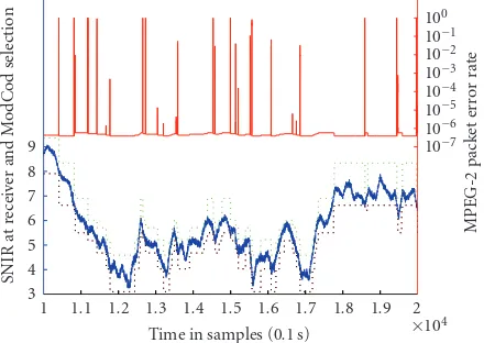
2
Figure12: PER with SNR and ModCod selection for zero-safety
margin.
Interarrival time of error bursts (event where PER>10−6) (s) 10−3
Probability density function for interarrival times
Figure13: Interarrival times distribution.
If a system can cope with these error rates, then it may be interesting to design it with lower safety margins than those in the W¨orz-Schweikert strategy, in order to gain throughput.
4.3. Error bursts analysis
To deeper investigate the quality of the transmission in case we reduce the safety margins, we have to look at the dis-tribution in time of the error bursts. Figure 12 shows an example of simulated SNR time series with corresponding PER for zero safety margin. In contrast toFigure 10which shows the averaged error PERs and BERs, here we investigate the distribution of the interarrival times between two PER peaks (without averaging), considering a detection threshold of PER=10−6. The simulation that has led toFigure 13has been worked out on 4.5 years of simulated SNR, and it was conducted with the zero-safety margins approach.
>0.5
We see that in 50% of cases, the time between two er-ror bursts is in the range of 0–100 seconds. This distribution comes from the fact that during a rain fade, ModCods are switched down one by one, and as we saw onFigure 12, error peaks often occur at every down-switch. The question is now what is the duration/severity of these peaks?
5. CONCLUSIONS
The possibility to have a quasi-error-free transmission chan-nel in DVB-S2 systems is not always an optimal solution in case the higher-layer protocols do not require such high per-formance. In this case the lower layers can provide a trans-mission with some resilient errors, and exploit more the spectrum to gain in throughput. The error-capacity trade-off can be tuned, according to the requirements of each partic-ular system, with the adjustment of the ModCod safety mar-gins. The paper presents the gain in spectral efficiency, which is obtained with this method, and the statistical characteris-tics of the “artificially” introduced error bursts, in terms of interarrival, duration and depth (PER). One additional in-teresting side-outcome of this work is the development of Markov chain to model the ModCod transitions and the fail-ure occurrence in a DVB-S2 system.
ACKNOWLEDGMENTS
This work was partly supported by EC funds SatNEx under the FP6 IST Programme, Grant number: 507052. This work was supported by the European Satellite Network of Excel-lence (SatNEx).
REFERENCES
[1] ETSI EN 302 307 V1.1.2, “Digital Video Broadcasting (DVB); second generation framing structure, channel coding and modulation systems for broadcasting, interactive services, news gathering and other broadband satellite applications,” June 2006.
[2] ETSI EN 301 790 V1.4.1, “Digital Video Broadcasting (DVB); interaction channel for satellite distribution systems,” April 2005.
[3] G. Fairhurst, M. Berioli, and G. Renker, “Cross-layer control of adaptive coding and modulation for satellite Internet multi-media,”International Journal of Satellite Communications and Networking, vol. 24, no. 6, pp. 471–491, 2006.
[4] ETSI TS 126 102, “AMR Speech Codec,” 2001.
[5] ISO/IEC 14496-2, “Coding of audio-visual objects (MPEG-4)—part 2: visual,” 2004.
[6] ETSI TR 126 975, “Performance Characterisation of the Adap-tive Multi-Rate (AMR) Speech Codec,” 2004.
[7] L.-A. Larzon, M. Degermark, S. Pink, L.-E. Jonsson, and G. Fairhurst, “The Lightweight User Datagram Protocol (UDP-Lite),” IETF, RFC 3828, 2004.
[8] S. Datta-Barua, P. H. Doherty, S. H. Delay, T. Dehel, and J. A. Klobuchar, “Ionospheric scintillation effects on single and dual frequency GPS positioning,” inProceedings of the 16th ternational Technical Meeting of the Satellite Division of the In-stitute of Navigation (ION GPS/GNSS ’03), pp. 336–346, Port-land, Ore, USA, September 2003.
[9] V. I. Tatarskii, Wave Propagation in a Turbulent Medium, McGraw-Hill, New York, NY, USA, 1961.
[10] E. Matricciani, M. Mauri, and C. Riva, “Relationship between scintillation and rain attenuation at 19.77 GHz,”Radio Science, vol. 31, no. 2, pp. 273–280, 1996.
[11] T. W¨orz, R. Schweikert, A. Jahn, and R. Rinaldo, “Physical layer efficiency of satellite DVB using fade mitigation tech-niques,” in Proceedings of the International Communication Satellite Systems Conference (ICSSC ’05), Rome, Italy, Septem-ber 2005.
[12] E. Casini, R. De Gaudenzi, and A. Ginesi, “DVB-S2 modem algorithms design and performance over typical satellite chan-nels,”International Journal of Satellite Communications and Networking, vol. 22, no. 3, pp. 281–318, 2004.