©IJRASET: All
Rights
are Reserved373
Automatic Generation Control of Two Area Linear
& Non Linear System using Teaching Learning
Optimization Technique
Sumit Paliwal1, Kapil Parikh2, Raunak Jangid3
1
M.tech Scholar, Assistant Professor2, Electrical Engineering, SITE, Nathdwara
Abstract: To increase affectivity of the generation system different power system share loads or it can said these are interconnected. It means different consumers at different places receiving power from multiple generators at different power stations. As all these power stations are interconnected via tie line the supplied power has to be regulated effectively. Also, the load side demands vary throughout the day which requires even more efficient and capable scheme to balance all the system by adjusting generator output. For this reason, we have Automatic Generation Control (AGC) system. This is achieved via continuous records frequency.
In the given work analysis of two area thermal-thermal non-reheat system has been carried out where its AGC system has been optimized. Here, the system is using PID controller for AGC utilizing Teacher Learner Based Optimization (TLBO) technique. Later the same scheme is used for non linear power system via the consideration of non linearity of Governor Dead Band (GDB). The whole model is developed in MATLAB/SIMULINK environment where it was studied and analyzed. The given work is described considering certain conditions to show its effectiveness. The operating load conditions, time constants of speed governor, turbine and tie line power (+50% to -50%) are these conditions under which system is analyzed. Also, the step change of load size and position is considered.
Previously, the system AGC has been optimized by the use of number for controllers based on various optimization techniques to improve the regulation of output power. Such as PI controller based on Hybrid Bacteria Foraging Optimization Algorithm-Particle Swarm Optimization (hBFOA-PSO) and Genetic algorithm. A comparison of results between the system with and without Governor Dead Band (GDB) has been presented to illuminate the matter more clearly. In case of without GDB the given scheme’s result is compared with hBFOA-PSO based schemes and with GDB the comparison is made between TLBO based and hBFOA-PSO based scheme only. Further the sensitivity of the system is also tested. It was tested by varying the system parameters and loading conditions at operating point form the nominal values.
Keywords: Automatic Generation Control; TLBO, hBFOA-PSO, GA Algorithm; Load Frequency Control;GDB
I. INTRODUCTION
A. Introduction
When two or more power stations are connected together to share the generation and load demand then such a network is said to be an interconnected power system. As said the obvious reason to employ such a system is to cope for the day to day load demand of the consumer. It is not possible for any one system to satisfy the demands of such a large network of consumers. Therefore different types of power system are interconnected which then gather the huge amount of power for transmission at what is known to us as Electrical grid. There are many advantages of interconnected power system such as increase stability, lower generation cost, sharing of load, reducing congestion in transmission and a backup system.
All these different stations are connected through a tie line. Basically tie line connects an area to other area for power exchange or power sharing. To manage the power through these tie lines and what amount of power has to be generated by what number of generator machine in each area require continuous monitoring of certain parameters. These parameters are system load demand, frequency and the tie line flow (power flow). Automatic generation control (AGC) system a supervisory control system does this work. It regularly monitors the change in system frequency and tie line flow. Accordingly, calculate the amount of change in power generated is needed at an instant also know as Area Control Error (ACE) and then change the status of the working generator in each area. This will allow low ACE average time.
©IJRASET: All
Rights
are Reserved374
near to set operating values. Therefore a proper balance of nominal frequency is important between generation and load side considering the losses incurring. The main goal of AGC is to maintain the system frequency i.e. Load frequency control.
For AGC system many scheme has already came forward which has shown their effectiveness to control the frequency and tie line power within the set limits. These schemes have included the case of normal change of load while the normal operation and some small variations in the system operating conditions of system. There are number of methods on based on which AGC control schemes have been developed, name of the few are, neural network, fuzzy logic, Genetic Algorithm (GA), Particle swarm optimization (PSO) and Bacteria Foraging Optimization Algorithm (BFOA) etc. in the given scenario AGC control scheme uses a MATLAB/SIMULINK environment for developing a Teaching learning Based Optimization Technique (TLBO) based PID controller to satisfy the given objective. The system for demonstrations used is two area non-reheat thermal systems.
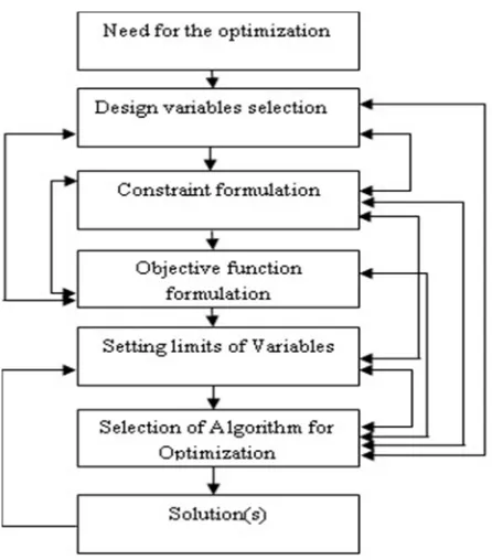
B. Objective Function
The objective function of the given system using PID controller is based on the constraints and specification. Performance index is used for the tuning of PID controller in case of closed loop responses. The specifications which are important for defining objective function are,
J =∫ (|∆f | + |∆f | + |∆P |). t. dt (1)
Hence the design problem of PID controller is stated as Minimize J subjected to
≤ ≤ , ≤ ≤ , ≤ ≤ (2)
II. SYSTEMMODEL
A. Block Diagram of (Two Area Thermal-Thermal System with No Reheat Turbine) Load Frequency Control
The system under study consists of two areas interconnected power system of non reheat thermal plant as shown in Fig.1 The system is extensively used in literature is for the design and analysis of automatic load frequency control of interconnected areas. They connected with tie line and different parameter represent by area1 and area 2 so area1 where f1 is the system frequency (Hz), R1 is the regulation constant (Hz/unit), TG1 is the speed governor time constant (s), TT1 is the turbine time constant (s) and TP1 is the
power system time constant (s), ACE1 is the area control error, ∆PD1 is the load demand change, ∆PC1 is the change in speed changer
position, ∆PG1 is the change in governor valve position, KP1 is the power system gain, and ∆Ptie is the change in tie line power and
where area2 where f2 is the system frequency (Hz), R2 is the regulation constant (Hz/unit), TG2 is the speed governor time constant
(s), TT2 is the turbine time constant (s) and TP2 is the power system time constant (s), ACE2 is the area control error, ∆PD2 is the load
demand change, ∆PC2 is the change in speed changer position, ∆PG2 is the change in governor valve position, KP2 is the power
system gain, As the obtain desire result, the PID controller consists of three essential modes, the proportional, the integral and the derivative modes. A proportional controller has the outcome of reducing the rise time, but never reduces the steady-state error. An integral control has the effect of reducing the steady-state error, but it may create the transient response poorer.
©IJRASET: All
Rights
are Reserved375
A derivative control has the effect of raising the stability of the system, drop PID the overshoot, and improving the transient response. The planned move toward is first applied to a linear two-area power system model without governor dead band linear system and then implement to a non-linear power system model by considering the effect of governor dead band non-linearity. As the call indicates, the PID algorithm consists of 3 basic modes, the proportional mode, the integral and the derivative A proportional controller has the effect of decreasing the rise time, but by no means removes the consistent-kingdom blunders. A necessary, manage has the effect of doing away with the consistent-country mistakes; however it can make the brief reaction worse.
B. Agc In Two Area System
In an single area system there are many generating machines couple internally so as to work with each other and cope up for the given load demand. Such an arrangement requires each and every system to run simultaneously and it is possible represent all the machine by the LFC loop. In case of two areas system, apart from the generators in the same area it is required that all the generating machines to be in synchronous irrespective of the area these are connected in. The real power transfer between the tie line of two area system,
P =| | | | sinδ (3)
(X =X1+Xtie+X2, δ = δ1+ δ2)
Tie line flow changes by small amount ΔP = Δδ = PΔδ = P (Δδ − Δδ ) (4)
III. TLBO TUNED PID CONTROLLER
A. Teaching Learning Optimization Technique
TLBO is the new kind of optimization algorithm for getting the more optimal operation of the problems, which have been previously, solved using other techniques. It is a very simple concept containing two important parts, one is a Teaching and other is learning.
It simulates the exact environment of a class room where a teacher is imparting knowledge to the students (learner). This is one way of learning as teacher knowledge is always more than the students. Then comes the second way, after teacher left the class room students start discussing the topic taught. Students will share with each their parts understanding of the topic that means interaction among them.
TLBO algorithm follows the same basic concept to find out the best possible solution in two parts,
1) Teacher (best solution) to students (learners)
2) Interaction among learners.
M(i)=mean
T(i)=teacher (best solution point)
Now T(i) will always works to move M(i) close to the value which it has. Therefore, now mean changes to Mnew. The new solution will be the difference of old and new mean.
Mean(i) = r(i) [Mnew TF×M(i)] (5)
r(i)=random no. (0 to 1)
TF =teaching factor ( 1 or 2 random selection). TF is responsible for the mean value change. Therefore, new solution is,
Xnew,(i) = Xold,(i) + Difference Mean(i) (6)
This is one part of learning directly via teacher. In other part learner learns via interaction among them. Learner learns from another learner only if the other has more knowledge. This update is given as,
I= no. of iteration For I = 1:Pn
Xi and Xj selected randomly I is not equal to j
If f (Xi) < f (Xj) Xnew(i) = Xold(i) + ri(Xi − Xj) (7)
Else Xnew(i) = Xold(i) + ri(Xj − Xi) (8)
Accept Xnew if it gives a better function value. Algorithm,
©IJRASET: All
Rights
are Reserved376
a) Statement of problem which is to be optimized. Initialization of parameters of it
Size of population =Pn Generation number= Gn
No. of Design Variables= Dn its limit (UL, LL). Ex.
Minimize f (X). Subject to Xi ∈ xi = 1, 2. . . Dn
f (X) =objective function, X = vector for design variables ( LL ≤ x(i) ≤ UL)
b) Starting P (Population).
Random generation of population depending on Pn and Dn. Here, Pn => learners
Dn => Subjects It is expressed as
P =
⎣ ⎢ ⎢
⎡ X , X, … . X ,
X , X , … . X ,
… . … . … . … .
X , X , … . X , ⎦
⎥ ⎥ ⎤
c) Teacher phase.
Mean calculation P column wise giving mean of each subject. M,D = [m1,m2, . . . ,mD]
For a iteration best solution is, Xteaxher=Xf (X)=min
Teacher efforts is to move M, D to Xteacher. This the new mean for the iteration. Mean Difference (i)= r(i) [Mnew TF×M(i)]
r(i) = random number (0≤r(i)≤1)
TF= teacher factor (0 to 1) decide new mean value Then the new solution is,
[image:4.612.191.414.463.717.2]Xnew, (i)= Xold, (i)+ Mean Difference (i) If function value is better accept Xnew.
©IJRASET: All
Rights
are Reserved377
d) Learner phase. learners increase their knowledge with the help of their mutual interaction
e) Termination criterion.
The given iteration will stop when Pn=maximum, otherwise goes to step 3.
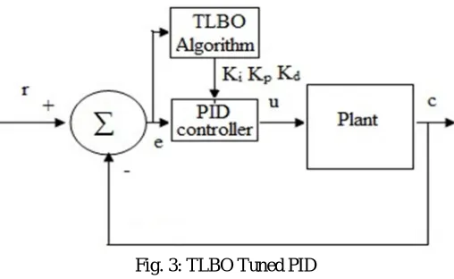
[image:5.612.180.434.136.292.2]B. TLBO tuned PID controller
Fig. 3: TLBO Tuned PID
Fig.3 shows TLBO tuned PID controller show.Based on teacher learner relationship PID controller parameters are modified. These modifications in the parameters depend upon the performance index. The performance index must be of minimum value. In a teacher learner relation teachers imparts knowledge of the subject to learners. The subject here are the parameters of controller which should have value close to or nearly equal to the best possible value i.e. optimal solution. There are namely three parameters Kp, Ki and Kd gain of PID controller.
IV. RESULT AND DISCUSSIONS
In this paper result, the effectiveness of the TLBO algorithm has been tested for Automatic Generation Control (AGC) of an interconnected power system. We used linear and nonlinear model of two area non-reheat thermal system equipped with Proportional-Integral derivative (PID) controller is considered initially for the design and analysis purpose. We use, a conventional Integral Time multiply Absolute Error (ITAE) based objective function is considered and the performance of TLBO algorithm is compared with hBFOA-PSO and GA. The contrast of Teaching Learning –Based Optimization (TLBO) is employed to look for optimum controller parameters to reduce the time domain objective feature. By means of contrast with the GA PID, hBFOA-PSO PID method and TLBO PID, the effectiveness of the proposed TLBO PID is verified over different running situations, and device parameters variations
A. MATLAB Model of SMIB System with SSSC Controller
Fig.4 shows MATLAB model of area-1and area-2 shows wiuthout governor dead band and various funnction act together as governor,turbine and power system with PID controller.
[image:5.612.66.558.555.718.2]©IJRASET: All
Rights
are Reserved378
B. Result of TLBO PID OptimizationTable 1: Controller Parameter of Different Technique without and with GDB
S.No. Parameters TLBO PID Controller Without GDB With GDB
1 Controller
Parameters
KP 6.6431 3.4145
KI 10 8.5449
KD 1.1004 1.0248
For the successful operation of TLBO it requires careful selection parameters
Fig. 5 shows the best cost function with an iteration of TLBO algorithm and its definitely the best value gets by TLBO algorithm
Fig.5: Convergence of Objective Function for gbest Load Frequency Control System
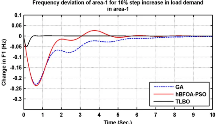
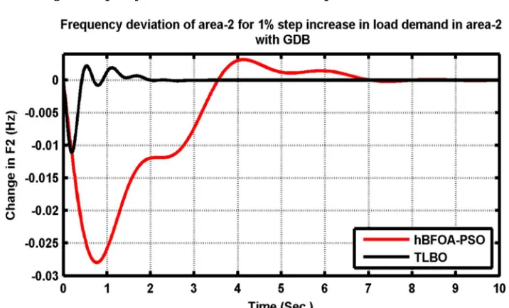
C. Frequency Deviation of Area-1, 2, for10% Step increase in Load demand in Area-1 & Area-2 with and without GDB
It is obvious from Figs.6 to 9 that, while Integral of Time multiplied Absolute Error (ITAE) is used for the objective function, the systematic presentation with proposed controller (TLBO PID) is superior to GA, hBFOA-PSO based PID controller with respect to ITAE criteria. The designed controllers are emphatic and carry out the satisfactory operation when employs TLBO PID controller.
[image:6.612.121.472.512.713.2]©IJRASET: All
Rights
are Reserved379
[image:7.612.117.472.303.480.2]Fig. 7: Frequency Deviation of Area-2 for 10% Step Increase in Load Demand in Area-2 without GDB
[image:7.612.115.473.495.712.2]Fig. 8: Frequency Deviation of Area-1 for 1% Step Increase in Area-1 with GDB
©IJRASET: All
Rights
are Reserved380
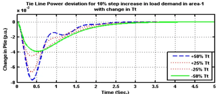
D. Sensitivity Analysis [image:8.612.125.473.182.352.2]The operating load condition and time constants of tieline power are diverse from their nominal values in the range of +50% to -50%. The time constants of tie-line power (T12),the time constants of speed governor (Tg),the time constant of turbine (Tt).are diverse from their nominal values in the range of +50% to -50% in steps of 25% taking one at a time. The power system parameters and time constants are computed for the various conditions and used in the simulation model. So it can achieve that, the proposed control approach implements a robust and stable control and need not be loaded for wider changes in the system loading or system parameters. The designed controllers are emphatic and carry out the satisfactory operation when employs TLBO PID controller
[image:8.612.108.509.384.533.2]Fig. 10: Frequency Deviation of Area-1 for 10% Step Increase in Load Demand in Area-1with Change in T12
Fig. 11: Frequency Deviation of Area-2 for 10% Step Increase in Load Demand in Area-1with Change in Tg
[image:8.612.126.488.560.716.2]©IJRASET: All
Rights
are Reserved381
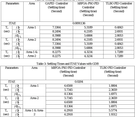
[image:9.612.77.535.107.505.2]Summarize finally conclude with various tables without GDB, sensitivity analysis, with GDB shown below
Table 2: Settling Times and ITAE Values without GDB
Parameters Area GAPID Controller
(Settling time) (Second) hBFOA-PSO PID Controller (Settling time) (Second)
TLBO PID Controller (Settling time)
(Second)
ITAE 0.0091136
Ts (sec)
∆ Area-1 7.3364 5.3189 0.4843
∆ 8.2494 6.2185 2.6931
∆ 8.3988 5.6806 2.8053
Ts (sec)
∆ Area-2 8.2494 6.2185 2.6931
∆ 7.3364 5.3189 0.4843
∆ 8.3988 5.6806 2.8053
Ts (sec)
∆ Area-1 &
Area-2
8.2275 4.3234 1.7289
∆ 8.2275 4.3234 1.7289
Table 3: Settling Times and ITAE Values with GDB
Parameters Area hBFOA-PSO PID Controller
(Settling time) (Second)
TLBO PID Controller (Settling time)
(Second)
ITAE 0.0204
Ts (sec)
∆ Area-1 6.6500 1.8804
∆ 5.7345 2.3659
∆ 8.1364 1.6971
Ts (sec)
∆ Area-2 5.7345 2.3659
∆ 6.6500 1.8804
∆ 8.1364 1.6971
Ts (sec)
∆ 1 &
Area-2
6.2918 5.5774
∆ 6.2918 1.9312
‘
Table 2 to 3 shows result without GDB, sensitivity analysis, with GDB with different operating conditions. Thesis work performs two stages, first tested to a linear two-area power system model and then continued to a non-linear power system model by as the effect of governor dead band non-linearity. The proposed algorithm TLBO-PID compare settling time with other recently reported algorithms like GA-PID, hBFOA-PSO for the similar power systems. An objective function using Time multiply Absolute Error (ITAE). The system shows better dynamic performance and improves system stability. Stability is improved and validated by different tables and graphs are shown below. Sensitivity analysis is performed by varying the system parameters and operating load conditions from their nominal values. Finally, we analysis system response all condition without GDB, with GDB and sensitivity analysis shows better response and satisfactory result.
V.CONCLUSIONS
©IJRASET: All
Rights
are Reserved382
REFERENCES
[1] H Erol, H Sezer and S Ayasun, "Computation of all stabilizing PI controller parameters of hybrid load frequency control system with communication time delay." In Smart Grid and Cities Congress and Fair (ICSG), 2017 5th International Istanbul, pp. 130-134. IEEE, 2017.
[2] A Zaidi and Q Cheng, "Online and offline load frequency controller design." In Power and Energy Conference (TPEC), IEEE Texas, IEEE, pp. 1-6, 2017. [3] H Parvaneh, SM Dizgah, M Sedighizadeh, and S T Ardeshir, "Load frequency control of a multi-area power system by optimum designing of frequency-based
PID controller using seeker optimization algorithm." In Thermal Power Plants (CTPP), 2016 6th Conference on, IEEE, pp. 52-57, Jan. 2016.
[4] MA Zamee, MM Hossain, A Ahmed and KK Islam, "Automatic generation control in a multi-area conventional and renewable energy based power system using differential evolution algorithm." In Informatics, Electronics and Vision (ICIEV), 2016 5th International Conference on, IEEE, pp. 262-267, 2016. [5] E Nikmanesh, O Hariri, H Shams and M. Fasihozaman, "Pareto design of load frequency control for interconnected power systems based on multi-objective
uniform diversity genetic algorithm (MUGA)," International Journal of Electrical Power & Energy Systems 80, pp. 333-346, 2016.
[6] RK Sahu, S Panda, A Biswal and GTC Sekhar, "Design and analysis of tilt integral derivative controller with filter for load frequency control of multi-area interconnected power systems," ISA transactions 61, pp. 251-264, 2016.
[7] S Kumari, G Shankar and S Gupta, "Study of load frequency control by using differential evolution algorithm." In Power Electronics, Intelligent Control and Energy Systems (ICPEICES), IEEE International Conference on, pp. 1-5. IEEE, 2016.
[8] S Kumari, G Shankar and Prince A, “Load Frequency Control Using Linear Quadratic Regulator and Differential Evolution Algorithm”, International Conference on Next Generation Intelligent Systems (ICNGIS), IEEE, pp. 1-5, 2016
[9] DK Lal, AK Barisal and SK Nayak, "Load frequency control of wind diesel hybrid power system using DE algorithm." In Intelligent Systems and Control (ISCO), 2016 10th International Conference on, IEEE, pp. 1-6, 2016.
[10] J Seekuka, R Rattanawaorahirunkul, S Sansri, S Sangsuriyan and A Prakonsant, "AGC using Particle Swarm Optimization based PID controller design for two area power system." In Computer Science and Engineering Conference (ICSEC), 2016 International, IEEE, pp. 1-4, 2016.
[11] RK Sahu, S Panda, UK Rout, DK Sahoo, "Teaching learning based optimization algorithm for automatic generation control of power system using 2-DOF PID controller", International Journal of Electrical Power & Energy Systems 77, pp. 287-301, 2016.
[12] GTC Sekhar, RK Sahu, A K Baliarsingh, and S Panda. "Load frequency control of power system under deregulated environment using optimal firefly algorithm." International Journal of Electrical Power & Energy Systems 74, pp.195-211, 2016.
[13] CK Shiva, V Mukherjee, "Design and analysis of multi-source multi-area deregulated power system for automatic generation control using quasi-oppositional harmony search algorithm", International Journal of Electrical Power & Energy Systems 80, pp. 382-395, 2016.
[14] LP Das, S Paul and PK Roy, "Automatic generation control of an interconnected hydro-thermal system using chemical reaction optimization", Michael Faraday IET International Summit: MFIIS-2015, pp. 77-6, Sept. 2015.
[15] RK Sahu, TS Gorripotu and S Panda, “A hybrid DE–PS algorithm for load frequency control under deregulated power systemwith UPFC and RFB ”, Ain Shams Engineering Journal, Elsevier, pp. 893-911, April 2015.