University of Pennsylvania
University of Pennsylvania
ScholarlyCommons
ScholarlyCommons
Technical Reports (CIS)
Department of Computer & Information Science
8-27-2009
Topics in Graph Construction for Semi-Supervised Learning
Topics in Graph Construction for Semi-Supervised Learning
Partha Pratim Talukdar
University of Pennsylvania
Follow this and additional works at: https://repository.upenn.edu/cis_reports
Recommended Citation
Recommended Citation
Partha Pratim Talukdar, "Topics in Graph Construction for Semi-Supervised Learning", . August 2009.
Topics in Graph Construction for Semi-Supervised Learning
Topics in Graph Construction for Semi-Supervised Learning
Abstract
Abstract
Graph-based Semi-Supervised Learning (SSL) methods have had empirical success in a variety of domains, ranging from natural language processing to bioinformatics. Such methods consist of two phases. In the first phase, a graph is constructed from the available data; in the second phase labels are inferred for unlabeled nodes in the constructed graph. While many algorithms have been developed for label inference, thus far little attention has been paid to the crucial graph construction phase and only recently has the importance of the graph construction for the resulting success in label inference been recognized. In this report, we shall review some of the recently proposed graph construction methods for graph-based SSL. We shall also present suggestions for future research in this area.
Comments
Comments
University of Pennsylvania Department of Computer and Information Science Technical Report No. MS-CIS-09-13.
Topics in Graph Construction for Semi-Supervised Learning
Partha Pratim Talukdar
University of Pennsylvania
[email protected]
August 27, 2009
Contents
1 Introduction 3 2 Problem Statement 43 k-Nearest Neighbor and -Neighborhood Methods 5
4 Graph Construction usingb-Matching (Jebara et al., 2009) 6
4.1 Graph Sparsification . . . 7
4.2 Edge Re-Weighting . . . 7
4.3 Results . . . 8
4.4 b-matching Complexity . . . 9
4.5 Discussion . . . 9
5 Graph Construction using Local Reconstruction (Daitch et al., 2009) 9 5.1 Hard Graphs . . . 9
5.2 α-Soft Graphs . . . 11
5.3 Properties of the Graphs . . . 11
5.4 Results . . . 12
5.5 Relationship to LNP (Wang and Zhang, 2008) . . . 12
6 Graph Kernels by Spectral Transform (Zhu et al., 2005) 12 6.1 Graph Laplacian . . . 13
6.2 Kernels by Spectral Transforms . . . 14
6.3 Optimizing Kernel Alignment . . . 15
6.5 Discussion . . . 17 6.6 Relationship to (Johnson and Zhang, 2008) . . . 17
7 Discussion & Future Work 17
8 Conclusion 19
Acknowledgment
I would like to thank my committee Mark Liberman, Ben Taskar (chair), and Lyle Ungar. Special thanks to Ted Sandler for many useful discussions.
Abstract
Graph-based Semi-Supervised Learning (SSL) methods have had empirical success in a variety of domains, ranging from natural language processing to bioinformatics. Such methods consist of two phases. In the first phase, a graph is constructed from the available data; in the second phase labels are inferred for unlabeled nodes in the constructed graph. While many algorithms have been developed for label inference, thus far little attention has been paid to the crucial graph construction phase and only recently has the importance of the graph construction for the resulting success in label inference been recognized. In this report, we shall review some of the recently proposed graph construction methods for graph-based SSL. We shall also present suggestions for future research in this area.
1
Introduction
Semi-Supervised Learning (SSL) methods can learn from labeled data combined with unlabeled data. While labeled data is hard and expensive to obtain, unlabeled data is often widely available. Because of this desirable property, SSL methods have received considerable attention in recent years (Chapelle et al., 2006). Graph-based SSL methods are particularly appealing because of their empirical success along with computational efficiency (Zhu et al., 2003; Zhou et al., 2004; Belkin et al., 2005; Bengio et al., 2007; Wang et al., 2008; Subramanya and Bilmes, 2008; Jebara et al., 2009; Talukdar and Crammer, 2009). Most of these methods are transductive in nature i.e. they can’t be used to classify an unseen test point in the future, though exceptions exist (Belkin et al., 2005). Graph-based SSL methods have been been effective in a wide variety of domains ranging from video recommendation (Baluja et al., 2008), protein classification (Tsuda et al., 2005) to assignment of semantic types to entities (Talukdar et al., 2008). Theoretical justification for graph-based methods is an area of active research (Lafferty and Wasserman, 2007; Niyogi, 2008; Singh et al., 2009).
Graph-based SSL methods operate on a graph where a node corresponds to a data instance and a pair of nodes are connected by a weighted edge. A few nodes in the graph are assigned labels. This initial supervision separates graph-based SSL methods from spectral clustering meth-ods (von Luxburg, 2007) which are unsupervised. Staring with this supervision, a graph-based SSL algorithm assigns labels to other unlabeled nodes in the graph. In most cases, the objective for label inference optimized by the algorithm results in an iterative process which amounts to spreading labels from the labeled to unlabeled nodes over the graph structure. Hence, graph-based SSL methods are sometimes also called Label Propagation methods. An alternative interpretation is to view these methods as performing random walks on the graph (Zhu et al., 2003; Baluja et al., 2008; Talukdar and Crammer, 2009).
As is evident from the discussion above, the graph on which learning is performed is a central object for any graph-based SSL method. In many real world domains (e.g. the web, social networks, citation networks, etc.), the data is relational in nature and there is already an implicit underlying graph. Graph-based methods are a natural fit in these domains. However, for a majority of learning tasks, the data instances are assumed to be independent and identically distributed (i.i.d.). In such cases, there is no explicit graph structure to start with. The common practice is to create a graph in the first step from independent data instances, and in the second step apply one of the graph-based SSL methods on the constructed graph. Even though graph-based SSL methods have been successfully applied to these tasks (Zhu et al., 2003; Subramanya and Bilmes, 2008), very
little attention has been given to the graph construction part, with majority of the research focus devoted to the post-graph construction learning algorithms. Only recently, importance of graph construction for resulting success in label inference has begun to be recognized (Maier et al., 2009; Wang and Zhang, 2008; Daitch et al., 2009; Jebara et al., 2009). In this survey, we shall review some of these methods for graph construction and also suggest opportunities for future research.
In Section 2, we shall present the notations and terminologies used throughout the report. Also, we shall present the assumptions common to all the methods reviewed.
In Section 3, we shall review two commonly used graph-construction methods: k-Nearest Neighbor (k-NN) and -neighborhood. We shall briefly look at their properties and also list ad-vantages of k-NN over-neighborhood.
In Section 4, we shall review the recently proposed method of graph construction using b -matching (Jebara et al., 2009). The idea will be to induce regular graphs where all nodes have the same degree (b). In contrast, popular methods like k-NN can generate irregular graphs. Through a variety of experiments, Jebara et al. (2009) argue for the importance of regular graphs for graph-based SSL methods. The graph construction process in (Jebara et al., 2009) involves two stages: in the first step a sparse graph is constructed where all edges have weight 1. In the second step, the edges are re-weighted using the Locally Linear Reconstruction (Roweis and Saul, 2000), among others.
In Section 5, we shall review another recently proposed method for graph construction (Daitch et al., 2009). In (Daitch et al., 2009), the concepts of Hard and α-Soft graphs are introduced. In case of hard graphs, each node is required to have a minimum weighted degree of 1. While, in case of α-soft graphs, this degree requirement is relaxed to allow some nodes (e.g. outliers) have lesser degree. Daitch et al. (2009) also analyze properties of the induced graphs, which is probably one of the first analyses of its kind. Effectiveness of these graphs in a variety of experiments are also presented in (Daitch et al., 2009) which we shall briefly review. We shall also explore the relationship between the method in (Daitch et al., 2009) to that of (Wang and Zhang, 2008).
In Section 6, we shall look at the method of kernel-alignment based spectral kernel design (Zhu et al., 2005). The idea here is to construct a kernel to be used for supervised learning, starting with a fixed graph and in the process transforming the spectrum of the graph Laplacian of the fixed graph. Though this is not exactly a graph construction method, it provides interesting insights into the graph Laplacian and its importance for graph-based SSL, which in turn may be exploited for graph construction. We shall also briefly look at the relationship between (Zhu et al., 2005) and (Johnson and Zhang, 2008). In (Johnson and Zhang, 2008), the relationship between graph-based SSL and standard kernel-based supervised learning is explored.
Finally, in Section 7, we shall analyze the methods further and also suggest promising direc-tions for future research.
2
Problem Statement
We are given a set of n points, X = {x1,x2, . . . ,xn}, sampled from a d dimensional space. We
shall interchangeably use the termspoints,instances and vectors. Each point has a length-c label vector associated with it, wherecis the total number of classes. The complete label set is given by
we are interested in inferring labels for the remainingn−l points,Xu={xl+1,xl+2, . . . ,xn}. As
mentioned in Section 1, graph-based methods operate on a graph where each point is associated with a node. In this report, we shall concentrate on the problem of constructing a graph on which the above mentioned methods could be applied to learn labels for the points inXu.
We shall represent the graph by G= (V, E, W), whereV is the set of nodes (|V|=n), E is the set of edges (|E|=m) andW is then×nedge weight matrix where weight of the edge (i, j) is given byWij. In the constructed graphG, the node corresponding to pointxi will be calledxi.
In such a graph, a weighted edge will connect two neighboring nodes. Unless otherwise stated, we shall assume the following:
• The induced graph is undirected and that all edge weights are non-negative i.e. Wij =Wji
andWij≥0, ∀i, j
• Wij= 0 indicates the absence of an edge between nodesiandj.
• There are no self-loops i.e. Wii = 0, ∀i= 1, . . . , n.
Given that the nodes (V) are fixed, the real problem is to learn the edge weight matrixW subject to the constraints above. Some of the methods surveyed may impose additional restrictions onW
which we shall specify as we go along.
3
k-Nearest Neighbor and
-Neighborhood Methods
k-Nearest Neighbors (k-NN) and -neighborhood are some of the most popular methods for con-structing a sparse subgraph from a set of points. Both methods assume availability of a similarity or kernel function using which similarity (or distance) between any two points in the data can be computed. In case of k-NN, undirected edges between a node and its k-nearest neighbors are greedily added. Finding the k-nearest neighbors in a naive way can be computationally expensive, specially in case of large datasets. However, a variety of alternatives and approximations have been developed over the years (Bentley, 1980; Beygelzimer et al., 2006).
In-neighborhood based graph construction, an undirected edge between two nodes is added only of the distance between them is smaller than, where >0 is a predefined constant. In other words, given a pointx, a ball (specific to the chosen distance metric) of radiusis drawn around it and an undirected edge between xand all points inside this ball are added.
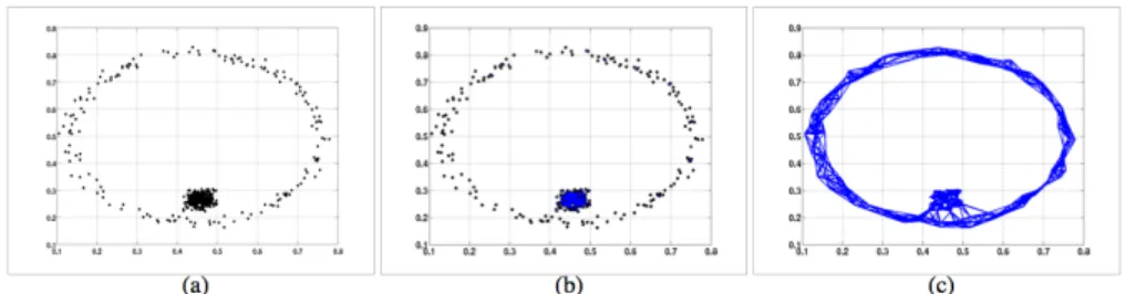
k-NN methods enjoy certain favorable properties compared to-neighborhood based graphs. For example, k-NN methods are adaptive to scale and density while an inaccurate choice ofmay result in disconnected graphs (Jebara et al., 2009). An empirical verification of this phenomenon on a synthetic dataset is shown in Figure 1. Also, k-NN methods tend to perform better in practice than-neighborhood based methods (Jebara et al., 2009). Recently, Maier et al. (2009) show that application of the same clustering algorithm (Normalized Cut, in this case) on two different graphs constructed using k-NN and-neighborhood may lead to systematically different clustering criteria.
Figure 1: k-NN and -neighborhood graphs constructed from a synthetic dataset (Jebara et al., 2009) (a) The synthetic dataset, (b) -neighborhood graph, (c) k-NN graph (k = 10). The -neighborhood is quite sensitive to the choice of and it may return graphs with disconnected components as in (b).
4
Graph Construction using
b
-Matching (Jebara et al., 2009)
As we had discussed previously in Section 3, k-NN methods are popular in constructing graphs. However, contrary to its name, k-NN methods often generate graphs where different nodes have different degrees. A node v can be in the k-nearest neighborhood of more than k nodes, which in itself results inv having degree greater than k. From example, consider Figure 2 which shows the 1-NN graph of a set of 5 points arranged in specific configuration. We note that the central node ends up with degree 4 which is significantly higher than degree 1 of all other four nodes. In order
Figure 2: 1-NN graph for a set of 5 points. Note that the central node ends up with degree 4 while all other nodes have degree 1, resulting in an irregular graph.
to induce a regular graph, a b-matching based graph construction process is proposed in (Jebara et al., 2009). b-matching guarantees a regular graph in which each vertex has exactlybdegree.
We shall use the same notations as in Section 2. The graph construction process outlined in (Jebara et al., 2009) can be decomposed into the following two steps:
• Graph Sparsification: Given a set of n points with similarity defined between each pair of points, a total of n2edges (undirected) are possible. This will result in a very dense graph
which can significantly slow down any subsequent inference on this graph. Hence, during graph sparsification a subset of the edges are selected which will be present in the final graph.
• Edge Re-Weighting: During this step, weights are learned for the edges selected in the sparsification step.
4.1
Graph Sparsification
Let k(·,·) be a kernel function used to measure similarity between two points. We define the similarity matrix A ∈ Rn×n where Aij = k(xi,xj). Note that A is a dense and symmetric (as k is symmetric). Sparsification removes edges by estimating a matrix P ∈B (B is the space of
{0,1}n×nmatrices) whereP
ij = 1 implies an edge between pointsxiandxj in the final graph and Pij = 0 implies absence of an edge between these two points in the final graph. We setPii = 0,
i.e. there are no self-loops. A symmetric distance matrixD ∈Rn×n can be constructed out of A
using the following transformation
Dij =
p
Aii+Ajj−2Aij
(Jebara et al., 2009) note that k-nearest neighbor can be viewed as a graph sparsification process which is optimizing the following optimization problem
minPˆ∈B
P
ijPˆijDij
s.t. P
jPˆij =k, Pˆii = 0, ∀i, j∈1, . . . , n
where the final binary matrix P is obtained by the symmetrization step: Pij = max( ˆPij,Pˆji).
Even though the optimization satisfies theP
jPˆij =kconstraint, the subsequent symmetrization
step only enforces the constraintP
jPij≥k, as we had discussed at the beginning of this section.
Sparsification by b-matching overcomes this problem by optimizing the following optimization problem
minP∈BPijPijDij
s.t. P
jPij =b, Pii= 0, Pij =Pji, ∀i, j∈1, . . . , n
Please note that the degree (P
jPij =b) and symmetrization (Pij =Pji) constraints are included
directly into the optimization and hence there is no need of any ad-hoc post-processing symmetriza-tion step as in the case of k-NN. Even though the change from k-NN tob-matching may seem quite trivial, there are significant differences in computation complexity. We shall discuss more about it in Section 4.4.
4.2
Edge Re-Weighting
With the set of edges selected through matrixP in the previous section, we would like to estimate the weights of the selected edges. In particular, we would like to estimate the symmetric edge weight matrixW with the following constraint: Wij ≥0 ifPij= 1 and Wij = 0 ifPij= 0. Three
• Binary (BN): In this case, we set W = P i.e. weights of all selected edges (Pij = 1)
are uniformly set to 1. This strategy may prevent recovery from errors committed during estimation ofP.
• Gaussian Kernel (GK): In this case, we set
Wij =Pijexp
−d(xi,xj)
2σ2
whered(xi,xj) measures the distance between pointsxiandxj, andσis a hyper-parameter. lp distance (Zhu, 2005),χ2 distance and cosine distance (Belkin et al., 2005) are some of the
choices ford(·,·).
• Locally Linear Reconstruction (LLR): This re-weighting scheme is based on the Locally Linear Embedding (LLE) technique (Roweis and Saul, 2000). Given the binary connectivity matrixP, weights of edges incident on nodexi (theWij’s) are estimated by minimizing the
following error
i=||xi−
X
j
PijWijxj||2
In this case, we would like reconstructxifrom its neighborhood information withPjPijWijxj
representing the reconstructed vector. The resulting optimization problem is shown below
minW Pi||xi−PjPijWijxj||2
s.t. P
jWij = 1, Wij≥0, i= 1, . . . , n
In (Jebara et al., 2009), it is claimed that the matrixW obtained from the above optimization is symmetric. However, with the symmetric constraint (Wij = Wji) not enforced during
optimization, it is difficult to see how that may be the case.
Anyways, With the edge weights (W) determined, we now have a weighted graph constructed on which any of the standard graph-based semi-supervised techniques e.g. Gaussian Random Fields (GRF) (Zhu et al., 2003), Local and Global Consistency (LGC) (Zhou et al., 2004) and Graph Transduction via Alternating Minimization (GTAM) (Wang et al., 2008) may be applied.
4.3
Results
Empirical evidence of importance of graph construction and its resulting effect on semi-supervised learning is presented in (Jebara et al., 2009). In particular, graph construction using following six combinations of sparsification and re-weighting methods are compared: { KNN, BM } × {
BN, GK, LLR }. For each constructed graph, three transductive learning methods: GRF, LGC and GTAM are compared against their label prediction accuracy on unlabeled nodes. In these experiments, all hyper-parameters (e.g. k, b, σ etc.) are heuristically set. Experimental results on synthetic and two real-world datasets are presented. From these results we observe that in most cases, b-matched graph improved performance compared to k-NN graph. Also, GTAM seems to be effective compared to GRF and LGC, with GRF and LGC achieving comparable accuracy.
4.4
b
-matching Complexity
While the greedy algorithm for k-NN is well known, complexity of the known polynomial time algorithm for maximum weightb-matching isO(bn3). Though recent advances in terms of loopy belief propagation has resulted in faster variants of it (Huang and Jebara, 2007). A sketch of the algorithm for bipartite graphs is shown in Appendix A of (Jebara et al., 2009).
4.5
Discussion
In (Jebara et al., 2009), the sparse matrixP is selected with one similarity measure while the edge re-weights are estimated with respect to another similarity measure (e.g. GK and LLR) resulting in a mismatch which may lead to sub-optimal behavior. It is worthwhile to consider learning both jointly using one similarity measure, and with some added penalty in favor of sparseness.
In (Jebara et al., 2009), the hyper-parameters are heuristically set which may favor one method or the other. In order to have a thorough comparison, a grid search over these parameters results based on those would have been more insightful. Also, Computational complexity is one of the major concerns for b-matching. It would have been insightful to have runtime comparison of
b-matching withk-NN.
As suggested in (Jebara et al., 2009), it will be interesting to see theoretical justification for the advantages ofb-matching, which is currently a topic of future research.
5
Graph Construction using Local Reconstruction (Daitch
et al., 2009)
Given a set of vectors (or points in high dimensional space) x1, . . . ,xn, (Daitch et al., 2009) ask
the question: what is the best graph that fits these points, where best is measured as per some fitness criteria? As an answer to this question, two types of graphs (Hard andα-Soft graphs), their properties and empirical comparison of these graphs to previously proposed graph construction methods are presented in (Daitch et al., 2009). We shall look into details of each of these in this section. We shall change the notations in (Daitch et al., 2009) as needed to make it consistent with previous sections of this report.
5.1
Hard Graphs
As per the definition in (Daitch et al., 2009), hard graphs are graphs where each node is strictly required to have (weighted) degree of at least 1. As before,W is the symmetric edge weight matrix where Wij =Wji≥0. Weighted degree,di, of a nodeiis defined as di=PjWij. Self loops are
not allowed and henceWii = 0, ∀i. Thehard graph construction algorithm presented in (Daitch
et al., 2009) minimizes the optimization problem shown in (1).
min W f(W) = X i ||dixi− X j Wijxj||2, s.t. di≥1, i= 1, . . . , n (1)
The degree constraints are necessary as an unconstrained minimization of f(W) will result in
Wij = 0, ∀i, j. We note thatf(W) is similar to the LLE (Roweis and Saul, 2000) objective when di = 1 ∀i. LLE pre-selcts the neighbors and allows non-symmetric edge weight matrix, where
some of the edge weights can be negative. In contrast, the graph construction method presented in Daitch et al. (2009) performs neighborhood selection and edge weighting in a single step, the edge weight matrix is symmetric and only non-negative edge weights are allowed. We shall now look at an algorithm to solve (1).
Letwbe a vector representation of the weight matrixW1, with only positive weighted edges considered. Note that whileW is of size n×n,w is a vector of lengthm as we consider only the edges currently present in the graph i.e. edges with positive weight. LetU be an×mmatrix with
Uie= 1 and Uje=−1 for eache= (i, j)∈E. LetV be am×m diagonal matrix with
diag(V) =w
Matrix V’s diagonal stores weights of all the edges in E. Let x(k) be the kth column of the n×d data matrix X whose ith row represents xi. We define the vector z(k) =UTx(k) and its
corresponding matrixZ= diag(z(1), . . . , z(d)). The Laplacian of the constructed graph,L, may be
decomposed as L=U V UT. f(w) (same as f(W) sincew is nothing but reshaped W) may now
be re-written as f(w) = ||LX||2 F = d X k=1 ||Lx(k)||2= d X k=1 ||U V UTx(k)||2 = d X k=1 ||U V y(k)||2= d X k=1 ||U Y(k)w||2=||Mw||2 whereMT = Y(1)UT, . . . , Y(d)UT and||M||F = (PijMij2) 1
2 is the Frobenius norm. The resulting
optimization problem for hard graphs is shown below.
min
w f(w) =||Mw||
2, s.t. d
i≥1, i= 1, . . . , n (2)
The problem shown in (2) is a quadratic program in n2
variables (length ofw). This is because for the set ofn nodes, a total of n2
(undirected) edges are possible. Optimizing (2) for all these variables at once may be computationally infeasible (Daitch et al., 2009). Hence, an incremental (greedy) algorithm is presented in (Daitch et al., 2009). The idea is solve the quadratic program (2) initially for a small subset of edges and then incrementally new edges to the problem which would improve the hard graph, and in the process remove any edge whose weight has been set to zero. This process is repeated until the graph can’t be improved any further. New edges to be added to the program are determined based on violation of KKT conditions (Nocedal and Wright, 1999) of the Lagrangian.
Some more details of this incremental algorithm (e.g. how to choose the initial set of edges etc.) would have helped in improving our understanding of it (Daitch et al., 2009).
5.2
α
-Soft Graphs
Sometimes it may be necessary to relax the degree constraint for some nodes. For example, we may want to have sparser connectivity for outlier nodes compared to nodes in high density regions. With this in mind, the degree constraint in (1) may be relaxed to the following
X
i
(max(0,1−di))2≤αn (3)
where αis a hyper-parameter. Graphs estimated with this new constraint will be called α-soft graphs. If all nodes satisfied the hard degree requirement (di ≥1 i.e. 1−di≤0, ∀i), then constraint
(3) is trivially satisfied. Eachhinge loss term, max(0,1−di), in the left hand side of (3) incurs a
positive penalty when the corresponding nodexi violates the degree constraint i.e. di <1. Note
that the value of f(w) = P
i||dixi−Pjwijxj||2 is decreased (improved) by uniformly scaling
down weights of all the edges. In that case, it is easy to verify that the constraint (3) will be satisfied with equality. If we defineη(w) =P
i(max(0,1−di)) 2, then
η(w∗) =αn (4)
wherew∗is a minimizer off(w) subject to constraint (3). Instead of incorporating constraint (3) directly, the algorithm for α-soft graphs in (Daitch et al., 2009) incorporates the constraint as a regularization term and instead solves the optimization problem shown in (5).
min
w f(w) +µ η(w), s.t.w≥0 (5)
whereµis a hyper-parameter. Let us now look at the algorithm forα-graph construction presented in (Daitch et al., 2009), which minimizes (5). Note that the objective in (5) is not directly dependent onα. We will see how that connection is established.
Letwbe a solution to (5) for some givenµ. In that case, following condition (4),w is also a solution for anα0-graph whereα0 = η(nw). Additionally, asµis increased,α0 decreases accordingly. This is because, asµis increased, the degree violation penalty,η(w), is going to be reduced as the objective in (5) is minimized. Hence, the algorithm starts with an initial guess forµwhich is then adjusted accordingly until α0 comes close toα(the desired value), subject to some tolerance. In this iterative algorithm, the problem in (5) is solved once for each value ofµ.
5.3
Properties of the Graphs
The hard and α-soft graphs may not be unique in general (Daitch et al., 2009). A few other properties of the hard and α-soft graphs are proved as well in (Daitch et al., 2009), which are reproduced below.
Theorem 3.1. For every α >0, every set of nvectors inRd has a hard and anα-soft graph
with at most (d+ 1)nedges.
This theorem suggests that the average degree (2nm) of any node in the graph is at most 2(d+1). For situations wherend, this theorem guarantees a sparse graph. Empirical validation of this is also presented in (Daitch et al., 2009). However, this bound will turn out to be very loose for high dimensional data e.g. data from Natural Language Processing where instances often have millions
of dimensions (or features). Daitch et al. (2009) also suggest that the average degree of a hard or
α-soft graph of a set of vectors is a measure of the effective dimensionality of those vectors, and that it will be small if they lie close to a low-dimensional manifold of low curvature. Currently, no theoretical (or empirical) validation of this claim is presented in (Daitch et al., 2009). However, if it were indeed the case, then such graph construction process may be independently useful in discovering dimensionality of a set of points in high dimensional space. This may also suggest whether methods like Manifold Regularization (Belkin et al., 2005) is going to be effective on such set of points.
Daitch et al. (2009) prove an additional theorem about planarity of induced hard and α-soft (α >0) graphs inR2.
5.4
Results
A variety of experimental results are presented in (Daitch et al., 2009) which demonstrate properties of the constructed hard and 0.1-soft graphs (α= 0.1) as well as their effectiveness in classification, regressions and clustering tasks. From Table 1 of (Daitch et al., 2009), it is interesting to note that the average degree of a node in the hard and soft graphs are lower than the upper bound predicted by Theorem 3.1. From the same table, we observe that hard and soft graph construction time increases sharply asnincreases, which raises scalability concerns for such methods.
Once the graphs are constructed, the label inference algorithm in (Zhu et al., 2003) used for classification and regressions experiments. Performance of hard and soft graphs are compared against k-NN and-neighborhood graphs. From the results in Tables 2 and 3 (Daitch et al., 2009), we note that inference on hard and 0.1-soft graphs outperform these other graph construction methods.
5.5
Relationship to LNP (Wang and Zhang, 2008)
The Linear Neighborhood Propagation (LNP) algorithm (Wang and Zhang, 2008) is a two step process whose step 1 involves a graph construction step. In this case, the graph is constructed by minimizing an objective (6) which is similar to the LLE objective (Roweis and Saul, 2000). As in Section 5.1, the difference with LLE is that in LNP, the edge weight matrixW is symmetric and that all edge weights are non-negative (these constraints are not shown in (6)).
min W X i ||xi− X j Wijxj||2, s.t. di= X j Wij = 1, i= 1, . . . , n (6)
By comparing (6) with (1) from Section 5.1, we note that the hard graph optimization enforces the constraintdi ≥1 while the LNP graph construction optimization (6) enforcesdi= 1. In other
words, LNP is searching a smaller space of graphs compared to hard graphs.
6
Graph Kernels by Spectral Transform (Zhu et al., 2005)
Graph based transductive methods often try to strike a balance betweenaccuracy(of the labeled nodes) and smoothness with respect to variation of labels over the graph. Smoothness enforces
the constraint that labels across a high weighted edge should not differ much. A central quantity in determining smoothness is the graph Laplacian, a matrix computed from edge weights. In (Zhu et al., 2005), it is noted that the eigenvectors of the graph Laplacian play a critical role in the resulting smoothness and that the eigenvectors can be combined using different weightings resulting in varying levels of smoothness. In (Zhu et al., 2005), such weightings of the eigenvectors of the graph Laplacian are called spectral transforms. A spectral transformation based method for estimating a graph kernel is presented in (Zhu et al., 2005), which will be discussed in this section. We first start with a review of the basic properties of graph Laplacian and its relationship to smoothness.
6.1
Graph Laplacian
Unnormalized Laplacian, L, of a graphG= (V, E) is defined as
L=D−W
where W is the symmetric edge weight matrix, andD is a diagonal matrix where Dii =PjWij
and Dij = 0 for i 6=j. We note that L, D, and W are all symmetric n×n matrices. Given a
function,f :V →R, which assigns scores (for a particular label) to each vertex inV, it is easy to verify that
fTLf = X
i,j∈V
Wij(f(i)−f(j))2 (7)
We note that minimization of Equation 7 enforces the smoothness condition as in such a mini-mization, we shall end up with f(i)≈f(j) for edges with highWij.
We know that Wij ≥ 0, ∀i, j and hence fTLf ≥ 0, ∀f which implies that L is a positive
semi-definite matrix. Letλ1≤λ2≤. . .≤λnand Φ1,Φ2, . . .Φn be the complete set of eigenvalues
and orthonormal eigenvectors of L. Smoothness penalty incurred by a particular eigenvector, Φi
is then given by
ΦTi LΦi=λiΦTiΦi=λi
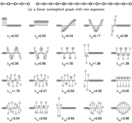
Thus, as noted in (Zhu et al., 2005), eigenvectors with smaller eigenvalues are smoother. For illustration, a simple graph (with two segments) and its spectral decomposition are shown in Figure 3. From this figure we observe the following,
• λ1=λ2= 0, which is equal to the number of connected components in the graph (in this case
2). In general, A graph haskconnected components iffλi= 0 fori= 1, . . . , k. Moreover, the
corresponding eigenvectors are constant within the connected components, which we observe in the first two plots of Figure 3 (b).
• The eigenvectors become more irregular with increasing eigenvalues.
This association between smoothness and ranked eigenvalues (and corresponding eigenvectors)will be exploited for learning smooth kernels over the graph is explained in next section.
Figure 3: A linear-chain graph (part (a)) with two segments and its spectral decomposition (part (b)). Note that the eigenvectors are smoother for lower eigenvalues (Zhu et al., 2005).
6.2
Kernels by Spectral Transforms
In order to learn a kernel K ∈ Rn×n which penalizes functions which are not smooth over the
graph, the following kernel form is considered in (Zhu et al., 2005)
K=X
i
µiφiφTi (8)
where φis are the eigenvectors of the graph LaplacianL, and µi≥0 are the eigenvalues of K. We
note that K is the non-negative sum of outer products and hence a positive semi-definite matrix and hence a valid kernel matrix. We wold like to point out that in order to estimateK, an initial graph structure is necessary as estimation ofKis dependent onLwhich is the Laplacian of a fixed graph.
In order to assign higher weight (µi) to outer product φiφTi of smoother eigenvectorφi (and
correspondingly smaller eigenvalue λi) of L, a spectral transformation function r : R+ → R+ is
follows
K=X
i
r(λi)φiφTi (9)
The spectral transformation essentially reverses the order of the eigenvalues. Construction of kernels from graph Laplacians have also been the focus of some previous research (Chapelle et al., 2002),(Smola and Kondor, 2003). For example, settingr(λi) =λi1+ (whereis a hyper-parameter),
results in the Gaussian field kernel used in (Zhu et al., 2003).
One remaining crucial question is the choice of function r. Although there are many natural choices, it is not clear up front which one is most relevant for the current learning task. Moreover, tuning any hyper-parameter associated with any parametric form ofr is another issue. In (Zhu et al., 2005), these issues are handled by learning a spectral transformation that optimizes kernel alignment to the labeled data 2. This is described in the next section.
6.3
Optimizing Kernel Alignment
LetKtrbe thel×lsub-matrix of the full kernel matrixK, withKtrcorresponding to thellabeled
instances x1, x2, . . . , xl. Let the l×l matrix T derived from the labels y1, y2, . . . , yl be defined
as: Tij = 1 if yi = yj and −1 otherwise. Empirical kernel alignment (Cristianini et al., 2001),
(Lanckriet et al., 2004) betweenKtr andT is defined as
A(Ktr, T) =
hKtr, TiF
p
hKtr, KtriFhT, TiF
(10)
where<·,·>F is the Frobenius product3. Please note thatA(Ktr, T) is maximized whenKtr∝T.
In (Zhu et al., 2005), the kernel matrix K (as given by Equation 8) is estimated by maximizing the kernel alignment objective in Equation 10, with the optimization defined directly over the transformed eigenvaluesµi, without any parametric assumption forrwhich would have otherwise
linked µi with the corresponding eigenvalue λi of L. Since the optimization is directly over the
variablesµi’s, we need a way to encode the constraint thatµiwith lower indexishould have higher
value (Section 6). In (Zhu et al., 2005), followingorder constraintsare added to the optimization to achieve this goal
µi≥µi+1, i= 1,2, . . . , n−1
The estimated kernel matrixKshould be a positive semi-definite matrix and hence the kernel alignment based optimization described above can be set up as a Semi-Definite Program (SDP). However, SDP optimization suffers from high computation complexity (Boyd and Vandenberghe, 2004). Fortunately, the optimization problem can also be set up in a more computationally efficient form. The resulting optimization problem is presented below
maxK A(Ktr, T)
subject to K=P
iµiφiφTi
Tr(K) = 1
2Please remember that the goal in (Zhu et al., 2005) is to learn a kernel in the (transductive) semi-supervised
setting and so a few instances are labeled. 3hM, Ni
µi≥0, i= 1,2, . . . , n µi≥µi+1, i= 1,2, . . . , n−1
The trace constraint is needed to fix the scale invariance of kernel alignment (Zhu et al., 2005). The problem can be equivalently rewritten as
maxK hKtr, TiF (11) subject to K=P iµiφiφTi (12) hKtr, KtriF ≤1 (13) µi≥0, i= 1,2, . . . , n (14) µi≥µi+1, i= 1,2, . . . , n−1 (15)
The kernel obtained by solving the above optimization is called Order Constrained Kernel (Zhu et al., 2005), which we shall denote byKOC. Another property of the Laplacian is exploited in (Zhu
et al., 2005) to define an Improved Order Constrained Kernel, which we shall refer to as KIOC.
In particular, λ1 = 0 for any graph Laplacian (Chung, 1997). Moreover, if there areno disjoint components in the graph then φ1 is constant overall4. In that case, φ1φT1 is a constant matrix
which does not depend onL, with the productµ1φ1φT1 acting as a bias term in the definition of K.
In that case constraint (15) from above can be replaced with
µi≥µi+1, i= 1,2, . . . , n−1, andφi not constant overall (16)
We would like to point out that constraint (16) is meant to affect onlyµ1and that too in connected
graphs only, as in all other casesφi is not going to be constant overall. Replacing constraint (15)
with (16) and solving the resulting optimization results in KIOC.
6.4
Results
Results from a large number of experiments comparing KOC and KIOC to six other standard
kernels: Gaussian (Zhu et al., 2003), Diffusion (Smola and Kondor, 2003), Max-Align (Lanckriet et al., 2004), Radial Basis Function (RBF), Linear and Quadratic. Out of these, RBF, Linear and Quadratic are unsupervised while the rest (including the proposed order kernels) are semi-supervised in nature. All 8 kernels are combined with the same Support Vector Machine (SVM) (Burges, 1998). Accuracy of the SVMs on unlabeled data is used as the evaluation metric. Experi-mental results from 7 different datasets are reported. For each dataset, an unweighted 10-NN (with the exception of one 100-NN) graph is constructed using either Euclidean or cosine similarity. In all cases, the graphs are connected and hence constraint (16) is used while estimatingKIOC. Smallest
200 eigenvectors of Laplacians are used in all the experiments. For each dataset, 5 training set sizes are used and for each set 30 random trials are performed. From the experimental results presented in (Zhu et al., 2005), we observe that the improved order constrained kernel,KIOC, outperformed
all other kernels.
4Otherwise, if a graph haskconnected components, then the firstkeigenvectors are piecewise constant over the
6.5
Discussion
In the sections above, we reviewed the kernel-alignment based spectral kernel design method de-scribed in (Zhu et al., 2005). At one end, we have the maximum-alignment kernels (Lanckriet et al., 2004) and at the other end we have the parametric Gaussian field kernels (Zhu et al., 2003). The order-constrained kernels introduced in (Zhu et al., 2005) strikes a balance between these two extremes. In such spectral transformation based methods, it will be interesting to see how the resulting edge weights (W) vary with different spectral transformations.
6.6
Relationship to (Johnson and Zhang, 2008)
In (Zhu et al., 2005) and its review in the sections above, we have seen how to derive a kernel from the graph Laplacian and effectiveness of the derived kernel for supervised learning. Johnson and Zhang (2008) look at the related issue of the relationship between graph-based semi-supervised learning and supervised learning. Let k be a given a kernel function and K the corresponding kernel matrix. LetL=K−1be the Laplacian of a graph. In that case, in Theorem 3.1 of (Johnson and Zhang, 2008), it is proved that graph-based semi-supervised learning using LaplacianL=K−1
is the equivalent to a kernel-based supervised learner (e.g. SVM) with kernel functionk.
In (Zhu et al., 2005), spectrum of the Laplacian of a fixed graph is modified to compute a kernel. While in (Johnson and Zhang, 2008), the kernel is created up front using all the data and without need for any a-priori fixed graph structure.
7
Discussion & Future Work
In this section we further analyze the methods reviewed in this report and suggest steps for future work.
• Degenerate Solutions: Graph-based SSL methods may generate degenerate (or trivial) solutions sometimes i.e. solutions where all nodes in the graph are assigned the same label. In order to handle this issue, various heuristics e.g. Class Mass Normalization (CMN) (Zhu et al., 2003) have been proposed. In CMN, class proportion information is taken into account account and the unlabeled points are classified so that the output class proportions are similar to the input class proportion. This is done by post-processing the output obtained from the graph-based SSL method.
From Section 6.1, we know that the eigenvectors corresponding to the smaller eigenvalues are smoother and in particular cases constant across each connected component. It will be quite insightful to explore the relationship between spectrum of the Laplacian and the possibility for degenerate solutions in a given graph. For a given algorithm, it will be useful to know the types of graphs on which it is likely to produce degenerate solutions so that more principled corrective steps can be taken accordingly. Transformation of the Laplacian may be one such possibility.
• Regular vs Irregular Graphs: Jebara et al. (2009) emphasize the importance of regular graphs (all nodes have same degree) for graph-based SSL compared to irregular graphs often
generated by popular graph-construction methods such as k-NN. It is not directly clear what effect node degrees have on the resulting classification. Inunder-regularized methods (Zhu et al., 2003), it is conceivable that presence of a high degree node may have adverse effect. In such cases, the algorithm may end up assigning most of the nodes the same label as the high degree node, thereby producing a degenerate solution as discussed previously. Recent methods have tried to address this problem by decreasing importance of high-degree nodes through additional regularization (Baluja et al., 2008; Talukdar and Crammer, 2009). In the light of these developments, it will be interesting to see whether the need for regular graphs can be substituted by applying these new regularized methods on corresponding irregular graphs.
• Construction based on Global Property: All the graph construction methods reviewed so far emphasize on local properties of the graph e.g. each node should have certain num-ber of neighbors (either exactly or approximately). There seems to be a lot more room for exploration in terms of enforcing other node local properties or even global properties (e.g. diameter of the graph). Enforcing global property directly may lead to combinatorial ex-plosion and so certain efficiently enforceable approximation of the global property may have to considered. Moreover, all induced graphs are undirected in nature. This is primarily be-cause graph-based transductive methods are targeted towards undirected graphs. However, transductive methods for directed graphs exist (Zhou et al., 2005) and so there is scope for induction of graphs with non-symmetric edge weight matrices.
• Alternative Graph Structures: All graph structures considered so far have instance-instance edges. There has been very little work in learning other types of graphs e.g. hybrid graphs with both features and instances present in them. Such types of graphs are used in (Wang, Z. and Song, Y. and Zhang, C., 2009), though the graph structure in this case is fixed a-priori and is not learned.
• Including Prior Information: All the graph construction methods surveyed so far (Jebara et al., 2009; Daitch et al., 2009; Wang and Zhang, 2008) use the locally linear reconstruction (LLR) principle (Roweis and Saul, 2000) in some way or the other. For example, (Daitch et al., 2009; Wang and Zhang, 2008) use variants of LLR during construction of the graph itself, while LLR is used for edge re-weighting in (Jebara et al., 2009). This suggests that there is room for exploration in this space in terms of other construction heuristics and methods. For example, none of these methods take prior knowledge into account. Sometimes we may know a-priori existence of certain edges and in the resulting graph we would like to include those edges. Such partial information may regularize the construction method and result in more appropriate graphs for the learning task at hand.
• Including Labeled Data: Unlike the empirical kernel alignment step in (Zhu et al., 2005), none of the graph construction methods (Jebara et al., 2009; Daitch et al., 2009; Wang and Zhang, 2008) exploit available labeled data during construction of the graph. This is related to the comment above about incorporation of prior-information. Labeled data may be seen as one type of prior information which could be useful in customizing the graph construction for the current learning task.
• New Application Settings: Most of the experimental datasets considered in the papers surveyed in this report have small number of instances and often small number of dimensions.
Since the methods reviewed can incorporate unlabeled data and acquiring unlabeled instances in most domains is often not hard, the number of instances input into the algorithms can be readily increased. Also, in many domains (e.g. Natural Language Processing), the number of dimensions (features) can run up to millions. It will be interesting to see effectiveness of these methods in such settings.
8
Conclusion
In this report, we have reviewed several recently proposed methods for graph-construction (Wang and Zhang, 2008; Jebara et al., 2009; Daitch et al., 2009). Locally Linear Reconstruction (Roweis and Saul, 2000) based edge weighting and enforcement of degree constraint on each node is a common theme in these methods. Daitch et al. (2009) further analyze properties of the induced graphs, while Jebara et al. (2009) emphasize the need for regular graphs in graph-based SSL. Additionally, we also looked at semi-supervised spectral kernel design (Zhu et al., 2005). Even though the graph structure is fixed a-priori in this case, this method highlights useful properties of the graph Laplacian and also demonstrates the relationship between the graph structure and a kernel that can be derived from it. Finally, we suggested a few steps for future work on graph construction for graph-based SSL.
References
S. Baluja, R. Seth, D. Sivakumar, Y. Jing, J. Yagnik, S. Kumar, D. Ravichandran, and M. Aly. Video suggestion and discovery for youtube: taking random walks through the view graph. Proceedings of WWW-2008, 2008.
M. Belkin, P. Niyogi, and V. Sindhwani. On manifold regularization. In Proc. of Conference on AI and Statistics, 2005.
Y. Bengio, O. Delalleau, and NL Roux. Semi-Supervised Learning, chapter Label Propogation and Quadratic Criterion, 2007.
J.L. Bentley. Multidimensional divide-and-conquer. Commun. ACM, 23:214–229, 1980.
A. Beygelzimer, S. Kakade, and J. Langford. Cover trees for nearest neighbor. In Proceedings of the 23rd international conference on Machine learning, pages 97–104. ACM New York, NY, USA, 2006.
S.P. Boyd and L. Vandenberghe. Convex optimization. Cambridge university press, 2004.
C.J.C. Burges. A tutorial on support vector machines for pattern recognition. Data mining and knowledge discovery, 2(2):121–167, 1998.
O. Chapelle, J. Weston, and B. Scholkopf. Cluster kernels for semi-supervised learning. InAdvances in Neural Information Processing Systems, 2002.
F.R.K. Chung. Spectral graph theory. Amer Mathematical Society, 1997.
N. Cristianini, J. Kandola, and A. Elissee. On kernel target alignment. Advances in Neural Information Processing Systems 14, 2001.
S.I. Daitch, J.A. Kelner, and D.A. Spielman. Fitting a graph to vector data. InProceedings of the 26th Annual International Conference on Machine Learning. ACM New York, NY, USA, 2009.
B. Huang and T. Jebara. Loopy belief propagation for bipartite maximum weight b-matching. Artificial Intelligence and Statistics (AISTATS), 2007.
T. Jebara, J. Wang, and S.F. Chang. Graph construction and b-matching for semi-supervised learning. In Proceedings of the 26th Annual International Conference on Machine Learning. ACM New York, NY, USA, 2009.
Rie Johnson and Tong Zhang. Graph-based semi-supervised learning and spectral kernel design. IEEE Transactions on Information Theory, 54(1):275–288, 2008.
J. Lafferty and L. Wasserman. Statistical analysis of semi-supervised regression. Advances in Neural Information Processing Systems, 20:801–808, 2007.
G.R.G. Lanckriet, N. Cristianini, P. Bartlett, L. El Ghaoui, and M.I. Jordan. Learning the kernel matrix with semidefinite programming. The Journal of Machine Learning Research, 5:27–72, 2004.
M. Maier, U. von Luxburg, and M. Hein. Influence of graph construction on graph-based clustering measures. The Neural Information Processing Systems, 22:1025–1032, 2009.
P. Niyogi. Manifold regularization and semi-supervised learning: Some theoretical analyses. Techni-cal report, TechniTechni-cal Report TR-2008-01, Computer Science Department, University of Chicago, 2008.
J. Nocedal and S.J. Wright. Numerical optimization. Springer, 1999.
S.T. Roweis and L.K. Saul. Nonlinear dimensionality reduction by locally linear embedding. Sci-ence, 290(5500):2323–2326, 2000.
A. Singh, R.D. Nowak, and X. Zhu. Unlabeled data: Now it helps, now it doesnt. InAdvances in Neural Information Processing Systems, 2009.
A.J. Smola and R. Kondor. Kernels and regularization on graphs. In Learning theory and Kernel machines: 16th Annual Conference on Learning Theory and 7th Kernel Workshop, COLT/Kernel 2003, Washington, DC, USA, August 24-27, 2003: proceedings, page 144. Springer Verlag, 2003.
A. Subramanya and J. Bilmes. Soft-Supervised Learning for Text Classification. InProceedings of EMNLP. Honolulu, Hawaii, 2008.
Partha Pratim Talukdar and Koby Crammer. New regularized algorithms for transductive learning. InECML-PKDD, 2009.
P.P. Talukdar, J. Reisinger, M. Pasca, D. Ravichandran, R. Bhagat, and F. Pereira. Weakly-Supervised Acquisition of Labeled Class Instances using Graph Random Walks. In Proceedings of the 2008 Conference on Empirical Methods in Natural Language Processing, pages 581–589, 2008.
K. Tsuda, H.J. Shin, and B. Scholkopf. Fast protein classification with multiple networks. Bioin-formatics, 21(90002), 2005.
U. von Luxburg. A tutorial on spectral clustering. Statistics and Computing, 17(4):395–416, 2007.
F. Wang and C. Zhang. Label propagation through linear neighborhoods. IEEE Transactions on Knowledge and Data Engineering, 20(1):55–67, 2008.
J. Wang, T. Jebara, and S.F. Chang. Graph transduction via alternating minimization. In Pro-ceedings of the 25th international conference on Machine learning, pages 1144–1151. ACM New York, NY, USA, 2008.
Wang, Z. and Song, Y. and Zhang, C. Knowledge Transfer on Hybrid Graph. InIJCAI, 2009.
D. Zhou, O. Bousquet, T.N. Lal, J. Weston, and B. Scholkopf. Learning with local and global consistency. InAdvances in Neural Information Processing Systems 16: Proceedings of the 2003 Conference, page 321. The MIT Press, 2004.
D. Zhou, J. Huang, and B. Scholkopf. Learning from labeled and unlabeled data on a directed graph. InICML, 2005.
X. Zhu. Semi-supervised learning literature survey. 2005.
X. Zhu, Z. Ghahramani, and J. Lafferty. Semi-supervised learning using gaussian fields and har-monic functions. ICML-03, 20th International Conference on Machine Learning, 2003.
X. Zhu, J. Kandola, J. Lafferty, and Z. Ghahramani. Graph kernels by spectral transforms. In Semi-Supervised Learning. MIT Press, 2005.