SPC for Software Reliability: Imperfect Software Debugging
Model
Dr. Satya Prasad Ravi1, N.Supriya2 and G.Krishna Mohan3
1
Associate Professor, Dept. of Computer Science & Engg., Acharya Nagrjuna University Nagarjuna Nagar, Guntur, Andhrapradesh, India
2
Assistant Professor, Dept. of Computer Science, Adikavi Nannaya university Rajahmedndry-533105, Andhrapradesh,India
3 Reader, Dept. of Computer Science, P.B.Siddhartha college Vijayawada, Andhrapradesh, India
Abstract
Software reliability process can be monitored efficiently by using Statistical Process Control (SPC). It assists the software development team to identify failures and actions to be taken during software failure process and hence, assures better software reliability. In this paper, we consider a software reliability growth model of Non-Homogenous Poisson Process (NHPP) based, that incorporates imperfect debugging problem. The proposed model utilizes the failure data collected from software development projects to analyze the software reliability. The maximum likelihood approach is derived to estimate the unknown point estimators of the model. We investigate the model and demonstrate its applicability in the software reliability engineering field.
Keywords: Statistical Process Control, Software reliability, mean value function, imperfect debugging, Probability limits, Control Charts.
1.
Introduction
Software reliability assessment is important to evaluate and predict the reliability and performance of software system, since it is the main attribute of software. To identify and eliminate human errors in software development process and also to improve software reliability, the Statistical Process Control concepts and methods are the best choice. SPC concepts and methods are used to monitor the performance of a software process over time in order to verify that the process remains in the state of statistical control. It helps in finding assignable causes, long term improvements in the software process. Software quality and reliability can be achieved by eliminating the causes or improving the software process or its operating procedures [6].
The most popular technique for maintaining process control is control charting. The control chart is one of the seven tools for quality control. Software process control is used to secure the quality of the final product which will conform to predefined standards. In any process, regardless of how carefully it is maintained, a certain amount of natural variability will always exist. A process is said to be statistically “in-control” when it operates with only chance causes of variation. On the other hand, when assignable causes are present, then we say that the process is statistically “out-of-control.”
The control charts can be classified into several categories, as per several distinct criteria. Depending on the number of quality characteristics under investigation, charts can be divided into univariate control charts and multivariate control charts. Furthermore, the quality characteristic of interest may be a continuous random variable or alternatively a discrete attribute. Control charts should be capable to create an alarm when a shift in the level of one or more parameters of the underlying distribution or a non-random behavior occurs. Normally, such a situation will be reflected in the control chart by points plotted outside the control limits or by the presence of specific patterns. The most common non-random patterns are cycles, trends, mixtures and stratification [7]. For a process to be in control the control chart should not have any trend or nonrandom pattern.
SPC is a powerful tool to optimize the amount of information needed for use in making management decisions. SPC provides real time analysis to establish controllable process baselines; learn, set, and dynamically improves process capabilities; and focus business areas
which need improvement. The early detection of software failures will improve the software reliability. The selection of proper SPC charts is essential to effective statistical process control implementation and use. The SPC chart selection is based on data, situation and need [4].
The control limits can then be utilized to monitor the failure times of components. After each failure, the time can be plotted on the chart. If the plotted point falls between the calculated control limits, it indicates that the process is in the state of statistical control and no action is warranted. If the point falls above the UCL, it indicates that the process average, or the failure occurrence rate, may have decreased which results in an increase in the time between failures. This is an important indication of possible process improvement. If this happens, the management should look for possible causes for this improvement and if the causes are discovered then action should be taken to maintain them. If the plotted point falls below the LCL, It indicates that the process average, or the failure occurrence rate, may have increased which results in a decrease in the failure time. This means that process may have deteriorated and thus actions should be taken to identify and causes may be removed. It can be noted here that the parameter a, b should normally be estimated with the data from the failure process.
The control limits for the chart are defined in such a manner that the process is considered to be out of control when the time to observe exactly one failure is less than LCL or greater than UCL. Our aim is to monitor the failure process and detect any change of the intensity parameter. When the process is normal, there is a chance for this to happen and it is commonly known as false alarm. The traditional false alarm probability is to set to be 0.27% although any other false alarm probability can be used. The actual acceptable false alarm probability should in fact depend on the actual product or process [9].
2.
Literature Survey
This section presents the theory that underlies a distribution and maximum likelihood estimation for complete data. If ‘t’ is a continuous random variable with pdf: f(t;1,2,,k) . where 1,2,,k are k unknown constant parameters which need to be estimated, and cdf: F
t . Where, The mathematical relationship between the pdf and cdf is given by:
dt t F d t f( ) . Let ‘a’ denote the expected number of faults that would be detected given infinite testing time in case of finite failure NHPP models. Then, the mean value function of the finite failure NHPP models can be written as:m(t) aF(t), where F(t) is a cumulative distribution function. The
failure intensity function (t) in case of the finite failure NHPP models is given by: (t) aF '(t).
2.1 NHPP model
The Non-Homogenous Poisson Process (NHPP) based software reliability growth models (SRGMs) are proved quite successful in practical software reliability engineering [3]. The main issue in the NHPP model is to determine an appropriate mean value function to denote the expected number of failures experienced up to a certain time point. Model parameters can be estimated by using Maximum Likelihood Estimate (MLE).
Various NHPP SRGMs have been built upon various assumptions. Many of the SRGMs assume that each time a failure occurs, the fault that caused it can be immediately removed and no new faults are introduced. Which is usually called perfect debugging. Imperfect debugging models have proposed a relaxation of the above assumption [8].
Let
N
t ,t 0
be the cumulative number of software failures by time ‘t’. m(t) is the mean value function, representing the expected number of software failures by time ‘t’.
t is the failure intensity function, which is proportional to the residual fault content. Thus
(1 bt) e a t m and
( ) b(a m(t)) dt t dm t .Where ‘a’ denotes the initial number of faults contained in a program and ‘b’ represents the fault detection rate. In software reliability, the initial number of faults and the fault detection rate are always unknown. The maximum likelihood technique can be used to evaluate the unknown parameters. In NHPP SRGM
t can be expressed in a more general way as
b
t
a t m
t
dt t dm
t ( )
.
Where a
t is the time-dependent fault content function which includes the initial and introduced faults in the program and b
t is the time-dependent fault detectionrate. A constant a
t implies the perfect debuggingassumption, i.e no new faults are introduced during the debugging process. If we assume that, when the detected faults are removed, then there is a possibility to introduce new faults with a constant rate ‘ ’. Then the mean value function is [2] given as m t a
e bt
1 1 1 ) ( .2.2 ML (Maximum Likelihood) Parameter Estimation
The idea behind maximum likelihood parameter estimation is to determine the parameters that maximize
the probability (likelihood) of the sample data. The method of maximum likelihood is considered to be more robust (with some exceptions) and yields estimators with good statistical properties. In other words, MLE methods are versatile and apply to many models and to different types of data. Although the methodology for maximum likelihood estimation is simple, the implementation is mathematically intense. Using today's computer power, however, mathematical complexity is not a big obstacle. If we conduct an experiment and obtain N independent observations,
t
1,
t
2,
,
t
N. Then the likelihood function is given by[1] the following product:
N i k i k N L f t t t t L 1 2 1 2 1 2 1, ,, | , ,, ( ; , ,, )Likely hood function by using λ(t) is:
L =
n i i t 1 ) ( The logarithmic likelihood function is given by:
N i k i t f L 1 2 1, , , ) ; ( ln ln Log L = log (
n i i t 1 ) ( ) which can be written as
n i n i m t t 1 ) ( ) ( log
The maximum likelihood estimators (MLE) of k
1, 2,, are obtained by maximizing L or
, where
is ln L . By maximizing , which is much easier to work with than L, the maximum likelihood estimators (MLE) of 1,2,,kare the simultaneous solutions of k equations such that:
0
j
, j=1,2,…,k
The parameters ‘a’ and ‘b’ are estimated using iterative Newton Raphson Method, which is given as
) ( ' ) ( 1 n n n n x g x g x x
3.
Illustrating the MLE Method
3.1 parameter estimation
To estimate ‘a’ and ‘b’ , for a sample of n units, first obtain the likelihood function: assuming 0.05 .
N i bt abe L 1 1 Take the natural logarithm on both sides, The Log Likelihood function is given as: Log L = log[ ( )] 1
n i i t
=
n i bt abe 1 1 ] log[ =
n i bt bte
a
abe
1 1 11
1
)
log(
Taking the Partial derivative w.r.t ‘a’ and equating to ‘0’. (i.e log 0 a L )
e btn
n a 1 1 1Taking the Partial derivative w.r.t ‘b’ and equating to ‘0’.
(i.e log 0 ) ( b L b g ) 1 0 1 1 1 1
n i i bt n t e t n b n b g n Taking the partial derivative again w.r.t ‘b’ and equating to ‘0’. (i.e log 0 ) ( ' 2 2 b L b g )
1
0 1 ' 2 2 1 1 2 2 b n e e t n b g n n bt bt n The parameter ‘b’ is estimated by iterative Newton Raphson Method using
) ( ' ) ( 1 n n n n b g b g b b . which is
substituted in finding ‘a’.
3.2 Distribution of Time between failures
Based on the inter failure data given in Table 1, we compute the software failures process through Mean Value Control chart. We used cumulative time between failures data for software reliability monitoring using Exponential distribution.
Table:1 Time between failures of a software
Failure Number Time between failure(h) Failure Number Time between failure(h) 1 30.02 16 15.53 2 1.44 17 25.72 3 22.47 18 2.79 4 1.36 19 1.92 5 3.43 20 4.13 6 13.2 21 70.47 7 5.15 22 17.07 8 3.83 23 3.99 9 21 24 176.06 10 12.97 25 81.07 11 0.47 26 2.27 12 6.23 27 15.63 13 3.39 28 120.78 14 9.11 29 30.81 15 2.18 30 34.19
Assuming an acceptable probability of false alarm of 0.27%, the control limits can be obtained as [5]:
1
0.99865 1 1 1 bt U e T
1
0.5 1 1 1 bt C e T
1
0.00135 1 1 1 bt L e T ‘ a ’ and ‘ b ’ are Maximum Likely hood Estimates (MLEs) of parameters and the values can be computed using iterative method for the given cumulative time between failures data shown in table 1. Using ‘a’ and ‘b’ values we can compute
m
(
t
)
.
These limits are converted to m(tU),m(tC)and m(tL) form. They are used to find weather the software process is in control or not by placing the points in Mean value chart shown in Figure 1. A point below the control limit
) (tL
m indicates an alarming signal. A point above the control limit m(tU)indicates better quality. If the points are falling within the control limits it indicates the software process is in stable condition [6]. The values of control limits are as follows.
31.69529
)
(
t
U
m
15.86907
)
(
t
C
m
0.042846
)
(
t
L
m
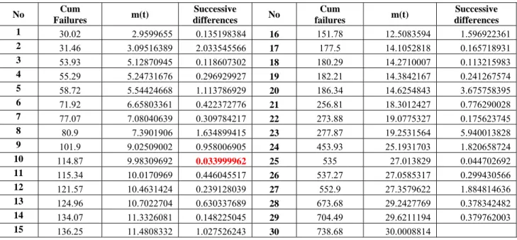
Table:2 successive differences of cumulative mean values
No Cum Failures m(t) Successive differences No Cum failures m(t) Successive differences 1 30.02 2.9599655 0.135198384 16 151.78 12.5083594 1.596922361 2 31.46 3.09516389 2.033545566 17 177.5 14.1052818 0.165718931 3 53.93 5.12870945 0.118607302 18 180.29 14.2710007 0.113215983 4 55.29 5.24731676 0.296929927 19 182.21 14.3842167 0.241267574 5 58.72 5.54424668 1.113786929 20 186.34 14.6254843 3.675758395 6 71.92 6.65803361 0.422372776 21 256.81 18.3012427 0.776290028 7 77.07 7.08040639 0.309784217 22 273.88 19.0775327 0.175623745 8 80.9 7.3901906 1.634899415 23 277.87 19.2531564 5.940013828 9 101.9 9.02509002 0.958006905 24 453.93 25.1931703 1.820658724 10 114.87 9.98309692 0.033999962 25 535 27.013829 0.044702692 11 115.34 10.0170969 0.446045517 26 537.27 27.0585317 0.299430566 12 121.57 10.4631424 0.239128039 27 552.9 27.3579622 1.884814636 13 124.96 10.7022704 0.630337689 28 673.68 29.2427769 0.378342482 14 134.07 11.3326081 0.148225045 29 704.49 29.6211194 0.379762003 15 136.25 11.4808332 1.027526243 30 738.68 30.0008814
Figure 1 is obtained by placing the differences between cumulative failure data shown in Table 2 on y axis, failure number on x axis and the values of control limits are placed on Mean Value chart. The Mean Value chart shows that the 10th failure data has fallen below
) (tL
m which indicates the failure process. It is significantly early
detection of failures using Mean Value Chart. The software quality is determined by detecting failures at an early stage. The remaining failure data are shown in Figure 1 are in stable. No failure data fall outside the
) (tU
UCL 31.695289517 CL 15.869068007 LCL 0.042846470 0.01000 0.04000 0.16000 0.64000 2.56000 10.24000 40.96000 1 2 3 4 5 6 7 8 9 10 11 12 13 14 15 16 17 18 19 20 21 22 23 24 25 26 27 28 29 su cc e ssiv e di ff e rences Date/Time/Period
Mean
Value
Chart
Figure: 1 Mean Value Chart
4.
Conclusion
The given 30 inter failure times are plotted through the estimated mean value function against the failure serial order. The parameter estimation is carried out by Newton Raphson Iterative method for Exponential model. The graphs have shown out of control signals i.e below the LCL. Hence we conclude that our method of estimation and the control chart are giving a +ve recommendation for their use in finding out preferable control process or desirable out of control signal. By observing the Mean value Control chart we identified that the failure situation is detected at 10th point of Table-2 for the corresponding
) (t
m , which is below m (tL ) . It indicates that the failure
process is detected at an early stage compared with Xie et a1, (2002) control chart [5], which detects the failure at 23rd point for the inter failure data above the UCL. Hence
our proposed Mean Value Chart detects out of control situation at an earlier instant than the situation in time control chart. The early detection of software failure will improve the software Reliability. When the time between failures is less than LCL, it is likely that there are assignable causes leading to significant process deterioration and it should be investigated. On the other hand, when the time between failures has exceeded the UCL, there are probably reasons that have lead to significant improvement.
References
[1] Hoang Pham, “Handbook Of Reliability Engineering”, Springer:Apr 2003, edition1.
[2] Huan-Jyh Shyur “A stochastic software reliability model with imperfect-debugging and change-point”- The journal of systems and software 66 (2003) 135-141.
[3] J.D. Musa., A. Iannino., K. Okumoto., 1987. “Software Reliability: Measurement Prediction Application”. McGraw-Hill, New York.
[4] J. F. MacGregor and T. Kourti “Statistical process control of multivariate processes”.
[5] M Xie, T.N Goh, P.Ranjan “Some effective control chart procedures for reliability monitoring” -Reliability engineering and System Safety 77 143 -150¸ 2002.
[6] M. Kimura, S. Yamada, S. Osaki.”Statistical Software reliability prediction and its applicability based on mean time between failures”.
[7] M.V.Koutras, S.Bersimis, P.E.Maravelakis “Statistical process control using shewart control charts with supplementary Runs rules” Springer Science + Business media 9:207-224, 2007.
[8] M.Ohba “Software Reliability Analysis Models” IBM Journal Research Development Vol.29,No. 4, pp. 428-442, July 1984.
[9] Swapna S. Gokhale and Kishore S.Trivedi, 1998. “Log-Logistic Software Reliability Growth Model”. The 3rd IEEE International Symposium on High-Assurance Systems Engineering. IEEE Computer Society.
Author’s profile:
First Author
Dr. R. Satya Prasad received Ph.D. degree in Computer Science in the faculty of Engineering in 2007 from Acharya Nagarjuna University, Andhra Pradesh. He received gold medal from Acharya Nagarjuna University for his out standing performance in Masters Degree. He is currently working as Associate Professor and H.O.D, in the Department of Computer Science & Engineering, Acharya Nagarjuna University. His current research is focused on Software Engineering. He has published several papers in National & International Journals.
Second Author
Mrs. N.Supriya Working as Assistant professor in the department of Computer Science, Adikavi Nannaya university, Rajahmedndry. She is at present pursuing Ph.D at Acharya Nagarjuna University. Her research interests lies in Softwrare Engineering and Data Mining.
Third Author
Mr. G. Krishna Mohan is working as a Reader in the Department of Computer Science, P.B.Siddhartha College, Vijayawada. He obtained his M.C.A degree from Acharya Nagarjuna University in 2000, M.Tech from JNTU, Kakinada, M.Phil from Madurai Kamaraj University and pursuing Ph.D at Acharya Nagarjuna University. His research interests lies in Data Mining and Software Engineering.