A Model Selection Approach for Expression Quantitative Trait Loci (eQTL) Mapping

(1)

CopyrightÓ2011 by the Genetics Society of America DOI: 10.1534/genetics.110.122796

A Model Selection Approach for Expression Quantitative

Trait Loci (eQTL) Mapping

Ping Wang,* John A. Dawson,* Mark P. Keller,

†

_{Brian S. Yandell,*}

,‡

_{Nancy A. Thornberry,}

§

Bei B. Zhang,

§

_{I-Ming Wang,}

§

_{Eric E. Schadt,}

§

_{Alan D. Attie}

†

_{and C. Kendziorski**}

,1 *Department of Statistics, University of Wisconsin, Madison, Wisconsin 53726,†Department of Biochemistry, University of Wisconsin,

Madison, Wisconsin 53726,‡Department of Horticulture, University of Wisconsin, Madison, Wisconsin 53726, **Department of Biostatistics and Medical Informatics, University of Wisconsin, Madison,

Wisconsin 53726 and§Merck, Whitehouse Station, New Jersey 08889 Manuscript received September 1, 2010

Accepted for publication November 7, 2010

ABSTRACT

Identifying the genetic basis of complex traits remains an important and challenging problem with the potential to affect a broad range of biological endeavors. A number of statistical methods are available for mapping quantitative trait loci (QTL), but their application to high-throughput phenotypes has been limited as most require user input and interaction. Recently, methods have been developed specifically for expression QTL (eQTL) mapping, but they too are limited in that they do not allow for interactions and QTL of moderate effect. We here propose an automated model-selection-based approach that identifies multiple eQTL in experimental populations, allowing for eQTL of moderate effect and interactions. Output can be used to identify groups of transcripts that are likely coregulated, as demonstrated in a study of diabetes in mouse.

M

ANY important problems in biology and medicine rely on the accurate identification of the genetic architecture underlying high-throughput phenotypes such as messenger RNA expression. Identifying expres-sion quantitative trait loci (eQTL) and grouping related traits are two primary goals addressed in such endeavors. This manuscript proposes an approach for eQTL mapping and shows how the derived transcript-specific genetic signatures can be used to group transcripts that are likely coregulated.

In the earliest eQTL mapping studies, simple single-QTL mapping methods were repeatedly applied to individual expression traits (Kendziorski and Wang

2006; Williamset al.2007) and that practice continues

today. Certainly powerful and effective methods that provide the flexibility to consider complex genetic models exist (Kao et al. 1999; Sen and Churchill

2001), and they have proven useful in numerous studies. However, the approaches require ‘‘fine tuning’’ (Sen

and Churchill2001) or the choice of thresholds (Kao et al.1999) to resolve multiple linked QTL and identify interactions for a single trait, and as a result applications to expression data are relatively few.

One of the first methods developed specifically for eQTL mapping was proposed by Storeyet al.(2005). In

that approach,F-statistics are calculated for each marker and trait, and a primary locus is identified for each trait as the one with a maximalF-statistic. A secondary locus is identified as the one having maximal statistic in a secondF-test conditional on the first, with permutations used to estimate the posterior probabilities and thresh-olds for locus-specific and joint linkage. Zouand Zeng

(2009) propose a sequential search for multiple QTL that combines features of Storey’s approach with MIM. Both approaches are automated and efficient and therefore useful in eQTL studies. However, the thresh-olding procedures in identification of primary and secondary loci may exclude potentially important traits affected by moderate and/or interacting QTL.

The methods discussed thus far all consider trait-specific tests or models, whereas some approaches model all traits (Kendziorskiet al.2006; Jiaand Xu2007) or

groups of traits (Chunand Kelesx2009) at once. With

one model for the data, it is possible to account for multiplicities and estimate false discovery rate across transcripts and markers simultaneously. However, the advantage gained is compromised at the level of inter-acting loci.

In summary, the state-of-the-art QTL mapping meth-ods are sophisticated and quite capable of identifying complicated genetic architecture, but most require that decisions on the class of models to consider, as well as significance thresholds, be made on a case-by-case basis.

Supporting information is available online athttp://www.genetics.org/

cgi/content/full/genetics.110.122796/DC1.

1_{Corresponding author:} _{Department of Biostatistics and Medical}

In-formatics, University of Wisconsin, 6729 Medical Sciences Center, 1300 University Ave., 6729 MSC, Madison, WI 53703.

E-mail: [email protected]

(2)

This clearly limits applications to studies of high-throughput phenotypes such as expression. Many of the challenges have been met to a great extent by the recently proposed methods designed specifically for eQTL mapping. However, these methods are unable to identify eQTL of small or moderate effect, and they do not allow for automated identification of interactions.

We here propose a new multiple-QTL mapping approach that has the ability to identify both QTL with large effect and those with small or moderate effect as well as interacting QTL. It is automated and efficient and therefore particularly well suited for eQTL studies. Our approach makes use of the results from a single-QTL analysis to reduce the marker search space and thereby reduce the model search space dramatically. The approach is detailed inA multiple-QTL identification approach allowing for interactions.

In addition to the multiple eQTL mapping approach, we propose a clustering method that incorporates eQTL mapping results and trait correlations to identify groups of transcripts that likely share similar biological func-tion. An early consideration of this problem is given in Eisen et al.(1998) in which investigators used

hierar-chical clustering applied to expression data to identify transcripts with similar function. To date, various clus-tering algorithms have been proposed in part to address this same goal (for a comprehensive review, see Doand

Choi 2007). A particularly powerful and popular

ap-proach was proposed by Zhangand Horvath(2005).

In their work, they describe a module identification approach that uses hierarchical clustering applied to a biologically meaningful distance derived from pairwise correlations between transcripts. When genetic data including genotypes and a genetic map are available in addition to expression data, ideally mapping informa-tion can be incorporated to improve the identificainforma-tion of groups of transcripts that are likely coregulated. To this end, inA model-based clustering method, we detail an approach that extends Zhangand Horvath(2005) to

include results from eQTL mapping in the identifica-tion of coexpression coregulaidentifica-tion (CECR) modules.

MATERIALS AND METHODS

A multiple-QTL identification approach allowing for interactions: Here, we propose a multiple-QTL mapping approach that has the ability to identify both QTL with large effect and QTL with small or moderate effect as well as interacting QTL. Motivation for our approach is based on the fact that multiple interacting loci induce marginal effects that can be detected by single-QTL mapping methods, as shown for two loci in Lanet al.(2001). Given this, the search space for models with first-order interactions can be dramatically re-duced. Instead of considering interactions between all markers, we focus on markers with relatively high LOD scores, even if those LOD scores are not statistically significant.

The multiple-QTL mapping approach uses preselected markers in a stepwise regression to identify main effects and interactions. Details follow for a single phenotype:

1. Obtain a LOD score profile by applying a single-QTL mapping method, such as interval mapping or Haley–Knott regression.

2. Preselect markers with relatively high LOD scores. Our approach for doing so is provided in the supporting information,File S1.

3. Perform stepwise regression to obtain a baseline model, one with main effects only. Candidates for main effects in this step are the preselected markers and relevant cova-riates (e.g., sex, age).

4. Perform stepwise regression to obtain the best model with interactions allowed. The potential interactions are be-tween the preselected markers or interactive covariates in the baseline model and all preselected markers.

In steps 3 and 4, a model selection criterion is needed. Many criteria take the form –2 logL 1 k3 c(n), where Lis the likelihood onn samples given a genetic model withk para-meters. For example,c(n)¼2 is the classical Akaike information criterion (AIC) (Akaike1974);c(n)¼ log(n) is the Bayesian information criterion (BIC) (Schwarz1978). The BIC is used in many studies, but as Bromanand Speed(2002) point out, its use can result in QTL models with many extraneous variables. Zouand Zeng(2008) discuss more conservative penalties such asc(n)¼2 log(n) andc(n)¼3 log(n), which we here refer to as BIC(2) and BIC(3), respectively. The recently proposed penal-ized LOD score (pLOD) criterion (Manichaikulet al.2009) could also be used.

A model-based clustering method: In eQTL studies, it is desirable to identify groups of coregulated traits that share similar biological function. Here we propose a clustering approach designed to accomplish this task. It incorporates both trait correlation and evidence of comapping. A measure-ment to quantify evidence in favor of comapping, as measured by the similarity of estimated mapping models, is introduced in the following.

Similarity between QTL models:For any pair of modelsM1,M2,

defined by the locations of QTL, M1¼ ðq11;q12;. . .;q1n1Þ

and M2¼ ðq21;q22;. . .;q2n2Þ, a similarity measure s should

satisfy the following two conditions: (i)s(M1,M2)2[0, 1] and

(ii)s(M,M)¼1 for allM.

Assume, without loss of generality, thatn1#n2. Letfpbe a

one-to-one mapping from f1;. . .;n1g to a subset of

f1;. . .;n2g with n1 elements; there are then P¼ n2n1 n1!

possible mappings [that is,fp(i)¼fp(j) impliesi¼j]. We

de-fine the model similarity to be

sðM1;M2Þ ¼ 2 n11n2

max

fp

Xn1

i¼1

cðq1i;q2fpðiÞÞ; wherecis a measure of similarity between two QTL,

cðq1;q2Þ ¼

1rðdÞ rðtÞ¼e

d=50_et=50

1et=50 ; ifq1;q2on the same chromosome andd¼ jq1q2j #m;

0; otherwise: (

m is a parameter set by the user that specifies the genetic distance within which two QTL can be considered similar;t$ mis a tuning parameter that quantifies the extent of similarity between two QTL within this distance. As t increases, the similarity between any two QTL within the window increases.

Supporting information, Figure S1 is a plot of similarity between QTLvs.distance between QTL in cM whenm¼2.5 cM for various tuning parameters. The choice of m is application dependent. When small genomic regions are of interest and dense maps and large sample sizes are available, two QTL that are 1 or 2 cM apart might not be considered similar. In such a case,mwould be chosen to be relatively small compared to situations in which larger regions are of interest

(3)

with fewer markers and samples. Oncemis specified, graphs such as that shown inFigure S1should be used to chooset.

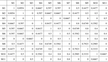
To examine some of the properties of the model similarity defined here, we calculated the similarities among 11 QTL models with 1, 2, and 3 QTL and provide them inTable S1

andTable S2. As shown there, the similarity measure is a function of QTL proximity between models as well as total number of QTL. Consider, for example, the similarity calculated between a modelM1that has a single QTL and

a series of nested QTL modelsM2,M5, andM9, whereM2,M5,

andM9each contain a QTL 0.5 cM from the QTL inM1.M5

andM9also contain one and two additional QTL,

respec-tively. The similarity measure maintains the following ordering: s(M1, M2) . s(M1, M5) . s(M1, M9). This is a

desired property since intuitively the similarity between two models should decrease as the number of discrepant loci increases.

Model-based clustering method: A measurement of the adja-cency between two traits that incorporates both correlation and mapping information is defined as

aij¼ jrijjsij;

whererijis the correlation between traitsiandjand

sij¼ s

ðMi;MjÞ; ifsðMi;MjÞ$s0

s0; otherwise:

Instead of directly usings(Mi,Mj) in the definition ofaij, we

usesijso that adjacencies are not zero necessarily for pairs of

traits whose model similarities equal 0. Such traits may still be related, and in this case we allow for the relationship to be

directly assessed by correlation. A choice for s0 iss0 ¼min

{s(Mi,Mj),s(Mi,Mj)6¼0}.

As in Zhangand Horvath(2005), we use average linkage hierarchical clustering coupled with the topological overlap matrix (TOM) distance to group traits into modules corre-sponding to branches of the hierarchical clustering tree (dendrogram). We extend their adjacency measure to the one given in a Model-based clustering method. Since it accom-modates both correlation and comapping, we refer to mod-ules constructed using this approach as CECR modmod-ules.

Enrichment test: Given a list of mapping transcripts, it is often of interest to determine whether the transcripts are enriched for any GO (gene ontology) terms in BP (biological process), CC (cellular component), MF (molecular function) categories, or KEGG (Kyoto Encyclopedia of Genes and Ge-nomes) pathways. The hypergeometric test implemented in the R package GOstats was used here for this purpose (R DevelopmentCoreTeam2009). The hypergeometric calcu-lation tends to result in smallP-values when groups with few transcripts are considered and as a result, it has been suggested that one consider only terms with smallP-values and a reason-able number of genes (10 or more) (Gentleman2004). Unless otherwise stated, we report terms withP-value,0.001, 10 or more genes on the chip, and 5 or more genes in the list annotated with that term.

DATA SETS CONSIDERED FOR EVALUATION To assess the proposed methodology we consider many individual traits from the QTL Archive, expression Figure1.—Adjusted BIC difference for QTL Archive studies. Positive (negative) absolute differences equal to or exceeding 10 units are highlighted in blue (red); absolute differences smaller than 10 units are highlighted in green.

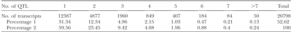
TABLE 1

The number of transcripts having 1,. . ., 7 and more than 7 main effects

No. of QTL 1 2 3 4 5 6 7 .7 Total

No. of transcripts 12387 4877 1960 849 407 184 84 50 20798

Percentage 1 31.34 12.34 4.96 2.15 1.03 0.47 0.21 0.13 52.62

Percentage 2 59.56 23.45 9.42 4.08 1.96 0.88 0.4 0.24 100

The percentages are given as percentages of the 39,524 transcripts (percentage 1) and the 20,798 mapping transcripts (per-centage 2).

(4)

traits collected in a study of diabetes, and simulated data. Details regarding each of these data sources follow.

QTL Archive studies: The QTL Archive (http:// churchill.jax.org/datasets/qtlarchive.shtml) created and maintained by the Jackson Laboratory (Bar Harbor, ME) provides access to raw data and result scripts from various QTL studies using rodent inbred line crosses. There were 31 studies in the QTL Archive as of June 29, 2008. The mapping method described inA multiple-QTL identification approach allowing for interactionswas applied to data from the QTL Archive. BIC was used for model selection, with results evaluated and compared using BIC, BIC(2), and BIC(3).

Microarray experiment: The C57BL/6J (B6) and BTBR mice are two inbred mouse populations main-tained at the Jackson Laboratory and often used in studies of type 2 diabetes. When made obese by a leptin mutation, B6 mice are diabetes resistant while the BTBR mice are diabetes susceptible (Cleeet al.2005). In this

study, expression profiles were obtained from 499F2 –

ob/ob mice generated from the C57BL/6J (B6) and BTBR founder strains. The profiles probed islet tissue using custom ink-jet microarrays manufactured by Agi-lent Technologies (Palo Alto, CA). The microarrays consisted of 1,048 control probes and 39,524 noncon-trol probes. Mouse islets were homogenized and total RNA extracted using Trizol reagent (Invitrogen, CA) according to the manufacturer’s protocol. Total RNA was reverse transcribed and labeled with flurochrome. Labeled complementary RNA (cRNA) from each animal was hybridized against a pool of labeled cRNAs con-structed from equal aliquots of RNA from all of the animals. All hybridizations were performed in fluor-reversal for 48 hr in a hybridization chamber, washed, and scanned using a confocal laser scanner. Expressions

were quantified on the basis of spot intensity relative to background, adjusted for experimental variation be-tween arrays using the average intensity over multiple channels, and fitted to a previously described error model to determine significance (type I error) (Heet al.

2003). Gene expression measures are reported as the ratio of the mean log10 intensity (mlratio). Plasma insulin levels were also measured in each of the 499 mice at approximately 10 weeks of age.

To ameliorate the effect of outliers, we performed a normal score transformation on the basis of ranks. In particular, for a trait (insulin level or expression trait) with measurements on n individuals, let Ri be the rank of

the measurement for individual i, and then the trans-formed measurement for individualiisyi¼F1(Ri/(n1

1)), where F1 _{is the inverse of the standard normal}

cumulative distribution function. All analyses in this diabetes study are based on the normal scores unless ex-plicitly stated otherwise. Mice were genotyped using the Affymetrix mouse 5K SNP panel (http://www.affymetrix.

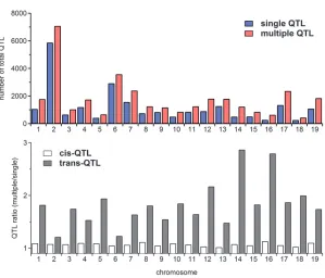
Figure 2.—Top: The total number of QTL (cis-QTL1 trans-QTL) identified by the single-and multiple-QTL mapping approaches. Bottom: Comparison between the number ofcis-QTL iden-tified by the multiple-QTL mapping approach and that identified using single-QTL mapping (open bars), and similarly fortrans-QTL (shaded bars).

TABLE 2

The number of transcripts mapping in 5-cM windows identified by the single and multiple-QTL analysis

(n.mapping.s and n.mapping.m, respectively)

Chr Pos (cM) n.mapping.s n.mapping.m

6 108.1 1978 2373

2 96.0 1578 1678

2 73.0 959 1592

2 89.2 796 984

7 4.0 495 890

12 8.0 402 843

17 8.4 621 778

Position of the window center is shown in centimorgans.

(5)

com); 1,953 SNPs on 19 autosomes reliably segregated for the founders and were used for QTL mapping.

RESULTS

QTL Archive studies: There were 31 studies in the QTL Archive as of June 29, 2008. To be included in our analysis, a study or trait had to satisfy the following conditions: (1) the data set provided in the QTL Archive had to match the description in the article; (2) the trait to be mapped had to be continuous and suitably handled by the normal model (perhaps following transformation); and (3) the markers closest to the identified QTL had to be given explicitly. This results in 24 traits in 11 studies (Clemenset al.2000; Farmeret al.2001; Ma¨ hleret al.

2002; Lyonset al.2003a,b and 2004a,b; Dipetrilloet al.

2004; Ishimoriet al.2004a,b; Korstanjeet al.2004). Figures S2–S12 and Tables S3–S13 compare the models derived using the proposed approach to those published. As shown in the figures, there is much similarity between models for regions with relatively high LODs. In particular, 67% (63%) of the loci

iden-tified in the published models with LODs exceeding 5.0 (4.0) are identified by the proposed approach; 80% (75%) are identified approximately (by markers within 5 cM of the published locus). The published models were also compared to those derived from the proposed approach using standard model selection criteria. Most of the QTL Archive studies derived models using the approach given in Senand Churchill(2001). As

pre-scribed there, a multiple imputation algorithm is used to fill in missing genotypes. When comparing models de-rived using the proposed approach to those published, differences due to randomness induced by imputing missing data are not of interest and, as a result, we com-pare models under two scenarios. The first considers a one-time imputation where each model is evaluated on the same set of imputed data; in the second we impute data 10 times, evaluate each set of imputed data, and report the median BIC. BIC* is the BIC obtained with missing genotypes filled in by a one-time imputation and BIC** is the median BIC.

Table S14lists BIC* and BIC** corresponding to the published model (superscript 1) and the model identi-fied using the proposed approach (superscript 2). The

TABLE 3

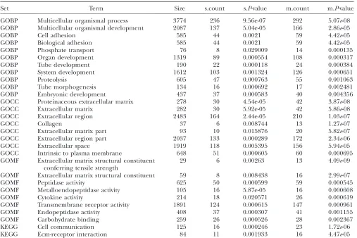
Results from an enrichment test applied to transcripts mapping to the 5-cM window centered at 108.1 cM on chromosome 6

Set Term Size s.count s.P-value m.count m.P-value

GOBP Multicellular organismal process 3774 236 9.56e-07 292 5.07e-08 GOBP Multicellular organismal development 2087 137 5.04e-05 166 2.86e-05

GOBP Cell adhesion 585 44 0.0021 59 4.42e-05

GOBP Biological adhesion 585 44 0.0021 59 4.42e-05

GOBP Phosphate transport 76 8 0.029009 14 0.000135

GOBP Organ development 1319 89 0.000554 108 0.000317

GOBP Tube development 190 22 0.000118 24 0.000384

GOBP System development 1612 103 0.001324 126 0.000651

GOBP Proteolysis 605 47 0.000763 55 0.001063

GOBP Tube morphogenesis 134 16 0.000692 17 0.002481

GOBP Embryonic development 437 37 0.000583 40 0.004356

GOCC Proteinaceous extracellular matrix 278 30 4.54e-05 42 3.87e-08

GOCC Extracellular matrix 282 30 5.92e-05 42 5.86e-08

GOCC Extracellular region 2483 164 2.44e-05 210 1.03e-07

GOCC Collagen 37 6 0.008744 13 1.27e-07

GOCC Extracellular matrix part 93 10 0.015876 20 5.82e-07

GOCC Extracellular region part 2037 133 0.000289 172 2.34e-06

GOCC Extracellular space 1919 118 0.005395 156 5.94e-05

GOCC Intrinsic to plasma membrane 648 51 0.000605 60 0.000695

GOMF Extracellular matrix structural constituent conferring tensile strength

29 6 0.00263 13 4.09e-09

GOMF Extracellular matrix structural constituent 59 8 0.008438 16 2.99e-07

GOMF Peptidase activity 625 50 0.000599 59 0.000545

GOMF Metalloendopeptidase activity 105 16 5.87e-05 16 0.000608

GOMF Cytokine activity 214 18 0.020571 26 0.000619

GOMF Transmembrane receptor activity 1891 124 0.000615 147 0.000961

GOMF Endopeptidase activity 408 37 0.000307 41 0.001155

GOMF Carbohydrate binding 259 26 0.000526 28 0.002367

KEGG Cell communication 125 16 0.000246 23 1.72e-06

KEGG Ecm-receptor interaction 84 11 0.001933 16 4.47e-05

Terms with size$10 andP-value#0.001 on either list from the single (s) and multiple (m)-QTL analysis are listed.

(6)

model complexity, indicated by (No. main effects, No. interactions), and missing genotype proportions are also given. As suggested by Kassand Raftery(1995),

we consider two models to be different if their corresponding BICs differ by more than 10 units. Both BIC* and BIC** suggest that the models identified by the proposed approach are comparable to published models when the amount of missing genotype data is small, and they may be advantageous in some cases. In particular, BIC* (BIC**) associated with the proposed approach is comparable (within 10 BIC units) to the BICs derived from published models for 7 of the 16 traits considered when the amount of missing data is less than 35%. For the 9 traits showing significant difference in BICs, the BICs derived from the proposed approach are smaller. However, when the proportion of missing genotype data exceeds 50%, the proposed approach performs rather poorly, showing comparable BICs in some cases and much larger BICs in others.

As shown in Figure 1, the same result holds generally when BIC(2) and BIC(3) are used. Figure 1 (left) shows the adjusted BIC difference between the two models for each trait as

BIC**;1BIC**;2 jBIC**;11BIC**;2j=2:

Similar plots are shown for BIC(2) (middle) and BIC(3) (right). The traits are ordered (top to bottom) by the proportion of missing genotypes (least to most), as in Table S14. Detailed numerical results for the BIC(2) and BIC(3) evaluations are given inTable S15

andTable S16, respectively.

The results here demonstrate that the models derived using the proposed automated approach largely overlap those found with other methods for regions with re-latively high LODs, and most often they show improve-ment as assessed by the BIC, BIC(2), and BIC(3) when the amount of missing genotype data is relatively small.

Diabetes study:This study considers anF2 intercross between B57BL/6 (B6) and BTBR mice to study type 2 diabetes. When made obese, B6 mice are resistant to diabetes, whereas BTBR are severely diabetic.

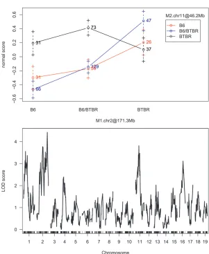
Identification of eQTL and comparison of methods: To identify eQTL and further reveal the genetic architec-ture underlying expression traits in islet tissue, we Figure 3.—Interaction plots and single-QTL LOD profiles for three expression traits. The LOD score for Cdk5rap1 (A) at rs4223605 (M1.chr2 at 156.7 Mb) is 42.37 and at rs13481837 (M2.chr13 at 60.1 Mb) is 14.6; the LOD score for Alkbh6 (B) at rs4226520 (M1.chr7 at 29.5 Mb) is 12.66 and at rs13479518 (M2.chr7 at 127.9 Mb) is 0.64; and the LOD score for Syn3 (C) at rs13476918 (M1.chr2 at 171.3 Mb) is 4.43 and at rs6365385 (M2.chr11 at 46.2 Mb) is 3.81.

(7)

applied two mapping approaches, a single-QTL mapping approach, and the multiple-QTL mapping approach detailed inA multiple-QTL identification approach allowing for interactions.

The single-QTL mapping approach used here is Haley–Knott regression (Haley and Knott (1992),

implemented in R/qtl (Bromanet al.2003). LOD score

profiles were obtained at a 2-cM resolution for each trait. For both insulin and the expression traits, sex was included as a main effect and an interactor. A cluster analysis of the 499 mice based on their expression profiles in islet indicated that not only sex but also the date on which the chips were run had effects on the expression measurements. Therefore, for expression traits, date was also included as a main effect. On each chromosome, the locus with maximum LOD score is claimed as a QTL if the LOD score is greater or equal to 5.0, which controls a genome-wide type-I error rate at 0.05.

The proposed approach was applied to each trait by first selecting markers with relatively high LOD scores from the Haley–Knott regression profiles. The variable search space was reduced dramatically since the num-bers of potential marker effects retained from 1,953

markers ranged from 46 to 83. Two stepwise regressions were then performed for model selection, as described in A multiple-QTL identification approach allowing for in-teractions, using pLOD as the model selection criterion (Manichaikul et al. 2009). As in the single-QTL

mapping analysis, sex was included as a main effect and a potential interactor for both insulin and the expression traits. For the expression traits, date was also included as a main effect. Table 1 summarizes the complexity of the models for expression traits in islet. In particular, 20,798 (52.62%) out of the 39,524 tran-scripts mapped to at least one QTL. Among the 20,798 mapping transcripts, 2 or more QTL were identified for 40.44% of the transcripts.

Although it is well known that a multiple-QTL mapping analysis is often advantageous over single-QTL mapping, a comparison is helpful to determine the particular advantages of the proposed approach. As expected, more eQTL are identified overall using the proposed approach (Figure 2, top). What is perhaps less expected is that the increase is almost entirely due to the identification of additional trans-acting eQTL (eQTL located outside a 5-cM window centered at the physical location of the

Figure3.—Continued.

(8)

expression transcript; see the Figure 2, bottom). In particular, the proposed approach identifies .92% of thecis-acting QTL (eQTL located within a 5-cM window centered on the physical location of the expression transcript) identified by the single-QTL mapping ap-proach along with a few others. It also identifies.80% of the trans-acting QTL identified by a single-QTL analysis and identifies 50% moretrans-acting QTL for most chromosomes.Table S17provides the total counts in detail.

A closer look considers the number of QTL within 5-cM windows. Table 2 lists the number of transcripts mapped by each method for several of the hottest win-dows. Notably, on chromosome 17, the hottest window (one with the most mapping transcripts) from the pro-posed approach is centered at 17 cM while the hottest window from the single-QTL analysis is centered at 8.4 cM. Interestingly, the transcripts mapped to 17 cM through the single-QTL analysis did not enrich for any GO BP terms, while those mapped by the proposed approach enriched for GO BP terms mitosis, M phase of mitotic cell cycle, M phase, and cell-cycle phase with

P-value , 0.001. Our group has recently detailed

evidence for the role of islet cell-cycle transcripts in diabetes (Kelleret al.2008).

Table 3 shows the results from an enrichment test applied to transcripts mapping to the window on chro-mosome 6; m.count and s.count are the numbers of genes annotated with the term among the list from the proposed approach and from a single-QTL analysis, respectively. For the 29 terms listed, m.count$s.count, and for 20 terms, m.P-value,s.P-value, suggesting gen-erally stronger enrichment results for transcripts iden-tified using the proposed approach.

As discussed earlier, one advantage of our proposed approach is the ability to identify interactions, particu-larly ones that involve moderate main effects. Among the 20,798 mapping transcripts, sex-by-marker or marker-by-marker interactions were identified for 7,985 (38.39%) transcripts. Among 8,411 transcripts mapping to 2 or more markers, 797 marker-by-marker interactions were identified across 763 transcripts. Figure 3 illustrates the types of interactions identified. The first part of Figure 3 highlights an interaction for which the main effect associated with each interacting term would have been found using the single-QTL approach; the second shows

Figure3.—Continued.

(9)

a case for which only one of the QTL would have been found; and the third shows a case in which neither locus is found significant in a single-QTL scan.

Insulin-based coexpression coregulation (CECR) module:

When eQTL colocalize with QTL of a clinical trait, one can hypothesize that a close relationship exists, such as sharing a regulator (Ferraraet al.2008). The

construc-tion of CECR modules has the potential to identify groups of traits that are likely coregulated, since both the correlation in expression along with mapping information is used. To illustrate, we consider the relationship between insulin and selected expression traits. First, the locations to which insulin maps were identified, where evidence of mapping was quantified, using the proposed approach. The model identified for insulin includes 7 QTL and two interactions, one between sex and marker rs3700924 (chromosome 17 at 8.4 cM) and the other between sex and marker rs13476801 (chromosome 2 at 91.7 cM). The 2,854 transcripts comapping with insulin were then identified as those with at least one locus in common. The pairwise similarities among the 2,855 traits (insulin and the comapping transcripts) were calculated using m ¼ 2.5 cM and t ¼ 5 cM, and CECR modules were con-structed. Figure 4 shows the resulting modules and the mapping patterns for the traits on the seven chromo-somes harboring insulin’s QTL. Columns are a series of 5-cM nonoverlapping bins along the seven chromo-somes and each row represents a trait. The much thicker top row highlights the model for insulin, with rows following the top row organized into CECR modules indicated by the colors on the far left. The (i,j)th entry is colored (not white) if theith transcript maps to the

jth genomic location as assessed by the proposed approach. The color used represents the single-QTL LOD score with LOD scores.5 shown in black. The top

row indicates that insulin maps to seven locations using the proposed approach, with two identified by single-QTL mapping.

Enrichment tests were performed to see whether the transcripts in the CECR modules are enriched for any biologically meaningful GO terms or KEGG pathways. The results are listed in Table S18. Insulin is in the turquoise module (a module with 540 transcripts), which enriches for innate immune response, a response known to be connected with insulin and diabetes (Ferna´ ndez-Real and Pickup 2008). In contrast, the

540 transcripts most correlated with insulin are en-riched only for wound healing, adult behavior, regula-tion of body fluid levels, and response to virus, none of which is particularly striking. From Figure 4, we see that most transcripts in the turquoise module have QTL near insulin’s QTL, rs13483664, at 36.8 cM (51 Mb) on chromosome 19. SorCS1 is one, located on chromo-some 19 between 50 and 51 Mb. In particular, the QTL model for SorCS1 involves rs13483664 and an interac-tion between sex and rs13483664. Clee et al. (2006)

have shown evidence suggesting that this gene has broad relevance to the development of type 2 diabetes.

DISCUSSION

Many important problems in biology and medicine rely on the accurate identification of QTL contributing to variation in quantitative traits. A number of powerful statistical methods for mapping QTL have proven useful in traditional mapping studies in which one or a few quantitative traits are surveyed. Typically, when thou-sands of phenotypes are available, as in an eQTL mapping study, single-QTL mapping methods are re-peatedly applied to individual expression traits, effec-Figure4.—The mapping patterns for insulin and the 2854 comapping transcripts. Columns are a series of 5-cM nonoverlapping bins across seven chromosomes harboring locations to which insulin maps. Shown are 2855 rows. The first represents insulin and is extra thick so that the locations to which insulin maps can be easily seen. There are 2854 rows following, one for each transcript, with row ordering determined by the CECR module construction. The color bar at the left represents the CECR modules. In-sulin is in the turquoise module. Bins containing QTL are colored (not white) with the color rep-resenting the magnitude of the LOD score ob-tained from a single-QTL analysis (LODs . 5 are colored black). In the rare event that a bin contains more than one QTL, the color corre-sponds to the maximum LOD score.

(10)

tively sacrificing the identification of refined genetic architecture for efficiency. We here propose an efficient and automated eQTL mapping approach that in part addresses this limitation, accommodating QTL of small or moderate effect as well as interactions. The output is used to identify CECR modules, groups of transcripts that are likely coregulated. In practice the approach could and likely should be applied following adjustment for latent variables or population structure such as in Leekand Storey (2007) and Kanget al.(2008). The

effects of doing so were not studied here.

The eQTL mapping approach consists of two-stage model selection over a reduced marker search space supported by the fact that interacting QTL induce effects that are detectable marginally. This motivates a first step of identifying markers with relatively large LOD scores following a single QTL scan. Model selec-tion is performed over the selected markers to de-termine a baseline model of main effects. A second model selection considers possible interactions. As noted, any one of several model selection criteria and procedures for identifying large LODs could be used. The approach results in the identification of a single model per transcript, which specifies the QTL affecting that transcript along with their actions and interactions. The model selection methods considered here have a number of advantages, but they do not target error-rate control and as a result no statements can be made regarding false discovery rates, for example, either within or across transcripts.

In the analysis of individual traits from the QTL Archive, the BIC was used for model selection since many of the published models utilize the BIC to some extent; models were evaluated using the BIC as well as BIC(2) and BIC(3). The results demonstrate that the proposed approach identifies models that largely over-lap those found with other methods for loci with large LOD scores, and in most cases they show improvement when there is not a large amount of missing genotype data (,35%). Here, improvement is assessed by de-creased BIC, BIC(2), and BIC(3), and of course in practice it is impossible to know which models better approximate reality. When consideration of one or a few phenotypes is of interest, as in the QTL Archive studies, clearly multiple approaches and lines of evidence should be considered during model development and selection. However, when high-throughput phenotypes prohibit such a careful and comprehensive evaluation, the automated approach proposed here can be useful.

As demonstrated in the diabetes case study, the output from the proposed approach can be used to identify groups of transcripts (or transcripts and clinical traits) that are likely coregulated. The so-called CECR module construction extends the definition of module initially proposed by Zhangand Horvath(2005) to

accommo-date trait-specific mapping information, in particular through the specification of a function that defines

model similarity. A specific form of model similarity was considered here, but could be modified through the choice of different tuning parameters and/or a different functional form. An investigation of different similarity measures should prove useful in guiding future applica-tions of CECR module construction as well as related efforts that require a measure of distance between two models. In this work, CECR module construction was used to identify groups of transcripts correlated and comapping with insulin. The groups generally show stronger enrichment for biological functions, suggesting improvement over using correlation measures alone.

This work was supported in part by the National Institute of General Medical Sciences (NIGMS) 76274, the National Institute of Diabetes and Digestive and Kidney Diseases (NIDDK) 66369, NIDDK 58037, and NIGMS training grant 74904.

LITERATURE CITED

Akaike, H., 1974 A new look at statistical model identification. IEEE

Trans. Automatic ControlAC-19:716–723.

Broman_{, K. W., and T. P. S}peed_{, 2002} _{A model selection approach} for the identification of quantitative trait loci in experimental

crosses. J. R. Statist. Soc. B64:641–656.

Broman_{, K. W., H. W}u_{, S. S}en_{and G. A. C}hurchill_{, 2003} _R/qtl:

QLT mapping in experimental crosses. Bioinformatics19:889–

890.

Chun, H., and S. Kelesx, 2009 Expression quantitative trait loci

map-ping with multivariate sparse partial least squares regression.

Genetics182:79–90.

Clee, S. M., S. T. Nadlerand A. D. Attie, 2005 Genetic and

geno-mic studies in the BTBR ob/ob model of type 2 diabetes. Am. J.

Ther.12:491–498.

Clee_{, S. M., B. S. Y}andell_{, K. M. S}chueler_{, M. E. R}abaglia_{, O. C.}

Richardset al., 2006 Positional cloning of a type 2 diabetes

quanitative trait locus. Nat. Genet.38:688–693.

Clemens_{, K. E., G. C}hurchill_{, N. B}hatt_{, K. R}ichardson_{and F. P.} Noonan, 2000 Genetic control of susceptibility to UV-induced immunosuppression by interacting quantitative trait loci. Genes

Immun.1(4): 251–259.

Di_Petrillo_{, K., S.-W. T}saih_{, S. S}heehan_{, C. J}ohns_{, P. K}elmenson

et al., 2004 Genetic analysis of blood pressure in C3H/HeJ

and SWR/J mice. Physiol. Genomics17(2): 215–220.

Do_{, J. H., and D. K. C}hoi_{, 2007} _{Clustering approaches to}

identi-fying gene expression patterns from DNA microarray data.

Mol. Cells25(2): 279–288.

Eisen, M. B., P. T. Spellman, P. O. Brown and D. Botstein,

1998 Cluster analysis and display of genome-wide expression

patterns. Proc. Natl. Acad. Sci. USA95:14863–14868.

Farmer, M. A., J. P. Sundberg, I. J. Bristol, G. A. Churchill, R. Li

et al., 2001 A major quantitative trait locus on chromosome 3 controls colitis severity in IL-10-deficient mice. Proc. Natl. Acad.

Sci. USA98(24): 13820–13825.

Ferna´ ndez_-Real, J. M., and J. C. Pickup, 2008 Innate immunity, in-sulin resistance and type 2 diabetes. Trends Endocrinol. Metab.

19(1): 10–16.

Ferrara, C. T., P. Wang, E. C. Neto, R. D. Stevens, J. R. Bainet al.,

2008 Genetic networks of liver metabolism revealed by

integra-tion of metabolic and transcripintegra-tional profiling. PLoS Genet.

4(3): e1000034.

Gentleman_{, R., 2004} _{Using GO for statistical analyses. In Compstat} 2004 Proceedings in Computational Statistics. Physica Verlag, Heidelberg, Germany.

Haley_{, C. S., and S. A. K}nott_{, 1992} _{A simple regression method for}

mapping quantitative trait loci in line crosses using flanking

markers. Heredity69:315–324.

He, Y. D., H. Dai, E. E. Schadt, G. Cavet, S. W. Edwards_{et al.},

2003 Microarray standard data set and figures of merit for

(11)

paring data processing methods and experiment designs.

Bioin-formatics19:956–965.

Ishimori, N., R. Li, P. M. Kelmenson, R. Korstanje, K. A. Walsh

et al., 2004a Quantitative trait loci analysis for plasma HDL-cholesterol concentrations and atherosclerosis susceptibility between inbred mouse strains C57BL/6J and 129S1/SvImJ.

Arterioscler. Thromb. Vasc. Biol.24:161–166.

Ishimori, N., R. Li, P. M. Kelmenson, R. Korstanje, K. A. Walsh

et al., 2004b Quantitative trait loci that determine plasma lipids and obesity in C57BL/6J and 129S1/SvImJ inbred mice. J. Lipid

Res.45:1624–1632.

Jia, Z., and S. Xu, 2007 Mapping quantitative trait loci for

expres-sion abundance. Genetics176:611–623.

Kang, H. M., C. Yeand E. Eskin, 2008 Accurate discovery of

expres-sion quantitative trait loci under confounding from spurious and

genuine regulatory hotspots. Genetics180:1909–1925.

Kao, C. H., Z.-B. Zengand R. D. Teasdale, 1999 Multiple interval

mapping for quantitative trait loci. Genetics152:1203–1216.

Kass, R. E., and A. E. Raftery, 1995 Bayes factors. J. Am. Statist.

Assoc.90:773–795.

Keller, M. P., Y. J. Choi, P. Wang, D. B. Davis, M. E. Rabagliaet al.,

2008 A gene expression network model of type 2 diabetes links

cell cycle regulation in islets with diabetes susceptibility. Genome

Res.18:706–716.

Kendziorski, C., and P. Wang, 2006 On statistical methods for

ex-pression quantitative trait loci mapping. Mamm. Genome17(6):

509–517.

Kendziorski, C., M. Chen, M. Yuan, H. Lan and A. D. Attie,

2006 Statistical methods for expression quantitative trait loci

(eQTL) mapping. Biometrics62:19–27.

Korstanje_{, R., R. L}i_{, T. H}oward_{, P. K}elmenson_{, J. M}arshall_{et al.}_,

2004 Influence of sex and diet on quantitative trait loci for

HDL cholesterol levels in an SM/J by NZB/BlNJ intercross

pop-ulation. J. Lipid Res.45:881–888.

Lan_{, H., C. M. K}endziorski_{, L. A. S}hepel_{, J. D. H}aag_{, M. A. N}ewton

et al., 2001 Genetic loci controlling breast cancer susceptibility

in the Wistar–Kyoto rat. Genetics157:331–339.

Leek, J. T., and J. D. Storey, 2007 Capturing heterogeneity in gene

expression studies by surrogate variable analysis. PLoS Genet.

3(9): 1724–1735.

Lyons, M. A., H. Wittenburg, R. Li, K. A. Walsh, G. A. Churchill

et al., 2003a Quantitative trait loci that determine lipoprotein cholesterol levels in DBA/2J and CAST/Ei inbred mice. J. Lipid

Res.44:953–967.

Lyons, M. A., H. Wittenburg, R. Li, K. A. Walsh, M. R. Leonard

et al., 2003b New quantitative trait loci that contribute to cho-lesterol gallstone formation detected in an intercross of CAST/Ei

and 129S1/SvImJ inbred mice. Physiol. Genomics14:225–239.

Lyons, M. A., R. Korstanje, R. Li, K. A. Walsh, G. A. Churchill

et al., 2004a Genetic contributors to lipoprotein cholesterol lev-els in an intercross of 129S1/SvImJ and RIIIS/J inbred mice.

Physiol. Genomics17:114–121.

Lyons, M. A., H. Wittenburg, R. Li, K. A. Walsh, R. Korstanje

et al., 2004b Quantitative trait loci that determine lipoprotein cholesterol levels in an intercross of 129S1/SvImJ and CAST/

Ei inbred mice. Physiol. Genomics17:60–68.

Ma¨ hler_{, M., C. M}ost_{, S. S}chmidtke_{, J. P. S}undberg_{, R. L}i_{et al.}_,

2002 Genetics of colitis susceptibility in IL-10-deficient mice:

backcross versus F2 results contrasted by principal component

analysis. Genomics80(3): 274–282.

Manichaikul_{, A., J. Y. M}oon_{, S. S}en_{, B. S. Y}andell _{and K. W.} Broman, 2009 A model selection approach for the identifica-tion of quantitative trait loci in experimental crosses, allowing

epistasis. Genetics181:1077–1086.

R DevelopmentCoreTeam, 2009 _{R: A Language and Environment}

for Statistical Computing.R Foundation for Statistical Computing, Vienna.

Schwarz_{, G., 1978} _{Estimating the dimension of a model. Ann.}

Stat-ist.6:461–464.

Sen_{, S., and G. A. C}hurchill_{, 2001} _{A statistical framework for}

quan-titative trait. Genetics159:371–387.

Storey_{, J. D., J. M. A}key_{and L. K}ruglyak_{, 2005} _{Multiple locus}

link-age analysis of genomewide expression in yeast. PLoS Biol.3(8):

e267.

Williams, R. B., E. K. Chan, M. J. Cowley and P. F. Little,

2007 The influence of genetic variation on gene expression.

Genome Res.17:1707–1716.

Zhang, B., and S. Horvath, 2005 A general framework for

weighted gene co-expression network analysis. Statist. Appl.

Genet. Mol. Biol.4:17.

Zou_{, W., and Z.-B. Z}eng_{, 2008} _{Statistical methods for mapping}

mul-tiple QTL. Int. J. Plant Genomics, 286561.

Zou_{, W., and Z.-B. Z}eng_{, 2009} _{Multiple interval mapping for gene}

expression QTL analysis. Genetica137:125–134.

Communicating editor: F. Zou

(12)

GENETICS

Supporting Information

http://www.genetics.org/cgi/content/full/genetics.110.122796/DC1

A Model Selection Approach for Expression Quantitative

Trait Loci (eQTL) Mapping

Ping Wang, John A. Dawson, Mark P. Keller, Brian S. Yandell, Nancy A. Thornberr y,

Bei B. Zhang, I-Ming Wang, Eric E. Schadt, Alan D. Attie and C. Kendziorski

(13)

P. Wang et al. 2 SI

File S1

0.0 0.5 1.0 1.5 2.0 2.5 3.0

0.0

0

.2

0.4

0

.6

0.8

1

.0

m = 2.5 cM

distance between QTL in cM

similarity between QTL

t = 2.5 cM t = 5 cM t = 10 cM t = 20 cM

t = Inf cM

FIGURE

S1: Similarity between QTL for

m

= 2

.

5 cM and various tuning parameters

t

≥

m

.

(14)

P. Wang et al. 3 SI

transformed % suppression

LOD

18.5 48.2 53 29 52 38 23.2 26

1 6 7 10 14 16 17 19

0.0

0

.5

1.0

1

.5

2.0

2

.5

3.0

chr

cM

FIGURE

S2: Vertical lines represent QTL: green lines for QTL identiﬁed by both methods; red

lines for QTL identiﬁed only by the proposed approach; blue lines for QTL in the published model

only. The height gives the LOD scores from a single QTL analysis. Two parallel axes, cM axis

and chr axis, are used for positioning a QTL. A QTL by QTL interaction is shown by connecting

the two points representing the two QTL, one on the cM axis and one on the chr axis. Red (blue)

(15)

P. Wang et al. 4 SI

GBV

LOD

15 16.5 29 15

2 3 5 7

01234

chr

cM

(16)

P. Wang et al. 5 SI

Non

HDL

LOD

43 19.5 24 9.2

8 14 15 20

0.0

1

.0

2.0

3

.0

chr

cM

Total Cholesterol

LOD

73 12.1 15 43 24 56.7

1 4 7 8 15 17 20

012345

chr

cM

(17)

HDL

LOD

81.6 86 74 43 26 22

1 2 6 8 9 12

02468

1

0

chr

cM

(18)

NonHDL

LOD

0.5 8 43 69

6 7 8 10 15

012345

chr cM

TG

LOD

57.4 68 41

4 9 14 18

01234

chr cM

% fat

LOD

67 43 68

1 6 8 9 12

02468

1

0

chr cM

BMI

LOD

101.2 43 5

1 8 17

0.0

0

.5

1.0

1

.5

2.0

2

.5

3.0

chr cM

(19)

P. Wang et al. 8 SI

Total Cholesterol

LOD

5

9

01234567

chr cM

NonHDL

LOD

5

9

012345

chr cM

HDL

LOD

48 21.9 46 71 3

2 4 6 14

01234567

chr cM

(20)

P. Wang et al. 9 SI

HDL0

LOD

92.3 53 18 20.5 47.7 42

1 3 5 6 15 16 18

02468

1

0

chr

cM

HDL6

LOD

101.5 68 25 34.3 57 41

1 5 8 9 17 18 19

02468

1

0

chr

cM

(21)

P. Wang et al. 10 SI

Cecum Total Score

LOD

61.8 13 32

3 8 18

05

1

0

1

5

chr

cM

Percentage of IgM+ B cells

LOD

49.7 18.8

3 8 17

02468

chr

cM

(22)

Blood Pressure

LOD

71.5 20 55 54.5

1 5 9 16

01234

chr

cM

(23)

P. Wang et al.

12 SI

Total Cholesterol

LOD

87.8 14 50 56.7

1 9 12 17

01234567

chr

cM

Non

HDL

LOD

56.7

17

01234

chr

cM

(24)

C.CecumPC1

LOD

55 33 36.5

3 8 16

0.0

0

.5

1.0

1

.5

2.0

chr cM

C.DistPC1

LOD

28 61.8 17 38 46.9

2 3 9 12 15

0.0

0

.5

1.0

1

.5

2.0

2

.5

3.0

chr cM

B.CecumPC1

LOD

41 45 20 16 30 36.5

3 5 6 11 12 13 16

0

.00

.5

1

.01

.5

2

.0

chr cM

B.MidPC1

LOD

64 38

10 12

01234

chr cM

B.DistPC1

LOD

45 74 36.5 54.6

5 6 16 17 19

0.0

0

.5

1.0

1

.5

2.0

chr cM

(25)

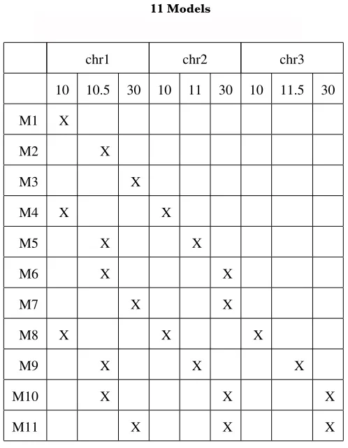
T

ABLE

S1: 11 models

chr1 chr2 chr3

10 10.5 30 10 11 30 10 11.5 30

M1 X

M2 X

M3 X

M4 X X

M5 X X

M6 X X

M7 X X

M8 X X X

M9 X X X

M10 X X X

M11 X X X

TABLE S1

11 Models

(26)

TABLE

S2: Similarity among models shown in TABLE

S1, with

m

= 2

.

5 cM and

t

= 5

cM.

M1 M2 M3 M4 M5 M6 M7 M8 M9 M10 M11

M1 1 0.8954 0 0.6667 0.597 0.597 0 0.5 0.4477 0.4477 0

M2 0.8954 1 0 0.597 0.6667 0.6667 0 0.4477 0.5 0.5 0

M3 0 0 1 0 0 0 0.6667 0 0 0 0.5

M4 0.6667 0.597 0 1 0.8437 0.4477 0 0.8 0.6749 0.3582 0

M5 0.597 0.6667 0 0.8437 1 0.5 0 0.6749 0.8 0.4 0

M6 0.597 0.6667 0 0.4477 0.5 1 0.5 0.3582 0.4 0.8 0.4

M7 0 0 0.6667 0 0 0.5 1 0 0 0.4 0.8

M8 0.5 0.4477 0 0.8 0.6749 0.3582 0 1 0.7923 0.2985 0

M9 0.4477 0.5 0 0.6749 0.8 0.4 0 0.7923 1 0.3333 0

M10 0.4477 0.5 0 0.3582 0.4 0.8 0.4 0.2985 0.3333 1 0.6667

M11 0 0 0.5 0 0 0.4 0.8 0 0 0.6667 1

TABLE S2

Similarity among models shown in TABLE S1, with m=2.5 cM and t= 5cM

(27)

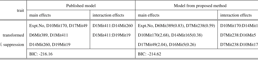
TABLES3: CLEMENSet al.(2000). There is no missing genotype data.

trait

Published model Model from proposed method

main effects interaction effects main effects interaction effects

Expt.No, D10Mit170, D17Mit49 D1Mit411:D14Mit260 Expt.No, D6Mit389(0.83), D7Mit238(0.59) D10Mit170:D14Mit165

transformed D6Mit389, D1Mit411 D1Mit411:D19Mit19 D10Mit170(2.68), D14Mit165(0.38) D7Mit238:D16Mit5

%suppression D14Mit260, D19Mit19 D17Mit49(2.04), D16Mit5(0.26) D7Mit238:D10Mit170

BIC: -216.16 BIC: -214.62

TABLE S3

CLEMENS et al. (2000). There is no missing genotype data

(28)

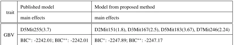
TABLES4: LYONSet al.(2003b).1.52%missing genotypes.

trait

main effects main effects

GBV

D5Mit255(3.7) D2Mit151(1.8), D3Mit167(2.5), D5Mit183(3.67), D7Mit246(2.24)

BIC∗: -2242.01; BIC∗∗: -2242.01 BIC∗: -2247.89; BIC∗∗: -2247.17

TABLE S4

LYONSet al. (2003b). 1.52% missing genotypes.

(29)

P. Wang et al.

18 SI

T

ABLE

S5: L

YONS

et al.

(2004b).

1 .

52%

missing genotypes. Note the means in Table 1 of L

YONS

et al.

(2004b) differ slightly

from those we calculated with the data provided.

trait

Non-HDL

D8Mit248, D15Mit115, DXMit81 D8Mit248(2.44), D14Mit260(2.50), D15Mit115(2.84), DXMit81(2.91)

BIC∗: 2366.63; BIC∗∗: 2372.06 BIC∗: 2364.71; BIC∗∗: 2370.12

Total

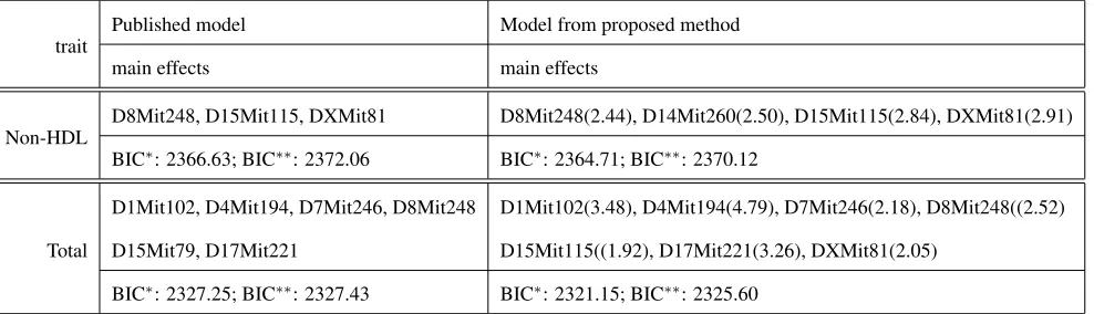
D1Mit102, D4Mit194, D7Mit246, D8Mit248 D1Mit102(3.48), D4Mit194(4.79), D7Mit246(2.18), D8Mit248((2.52)

D15Mit79, D17Mit221 D15Mit115((1.92), D17Mit221(3.26), DXMit81(2.05)

BIC∗: 2327.25; BIC∗∗: 2327.43 BIC∗: 2321.15; BIC∗∗: 2325.60

TABLE S5

LYONS et al. (2004b). 1.52% missing genotypes.

Note the means in Table 1 of LYONS et al. (2004b) differ slightly from those we calculated with the data provided.

(30)

T

ABLE

S6: I

SHIMORI

et al.

(2004a).

1 .

80%

missing genotypes.

trait

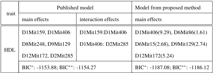
main effects interaction effects main effects

HDL

D1Mit159, D1Mit406 D1Mit159:D1Mit406 D1Mit406(9.29), D6Mit86(1.61)

D8Mit248, D9Mit129 D1Mit406: D2Mit285 D6Mit15(2.68), D9Mit129(2.74)

D12Mit172, D2Mit285 D12Mit172(5.24)

BIC∗: -1153.88; BIC∗∗: -1154.27 BIC∗: -1187.08; BIC∗∗: -1186.12

TABLE S6

ISHMORI et al. (2004a). 1.80% missing genotypes.

(31)

P. Wang et al.

20 SI

T

ABLE

S7: I

SHIMORI

et al.

(2004b).

2 .

38%

missing genotypes.

trait

Non-HDL

D8Mit248, D10Mit35 D8Mit248:D7Mit294 D8Mit248(4.06)

D7Mit294, D15Mit13 D10Mit35:D15Mit13

BIC∗: -1024.05; BIC∗∗: -1023.62 BIC∗: -1062.04; BIC∗∗: -1062.99

TG

D14Mit60, D4Mit308

BIC∗: 1465.47; BIC∗∗: 1465.76 BIC∗: 1440.55; BIC∗∗: 1440.55

%fat

D8Mit248,D12Mit182 D8Mit248:D9Mit281 D1Mit495(2.00)

D6Mit86, D1Mit495 D8Mit248(9.83)

D9Mit281 D12Mit84(2.74)

BIC∗: 1017.68; BIC∗∗: 1015.15 BIC∗: 997.37; BIC∗∗: 995.58

BMI

D17Mit143, D8Mit248 D1Mit406(2.38)

D1Mit406 D17Mit143(2.82)

BIC∗: -1714.00; BIC∗∗: -1713.99 BIC∗: -1717.80; BIC∗∗: -1717.38

TABLE S7

ISHMORI et al. (2004b). 2.38% missing genotypes.

(32)

T

ABLE

S8: L

YONS

et al.

(2003a).

2 .

63%

missing genotypes.

trait

Total

D9Mit58 D9Mit90(6.99)

BIC∗: 2467.99; BIC∗∗: 2467.99 BIC∗: 2464.15; BIC∗∗: 2464.15

Non-HDL

D9Mit58 D9Mit90(4.20)

BIC∗: 2462.30; BIC∗∗: 2462.30 BIC∗: 2462.92; BIC∗∗: 2462.92

HDL

D2Mit94, D4Mit110 Lineage, D2Mit94(5.97), D4Mit110(6.26)

D6Mit36, D6Mit14 D6Mit14(4.03), D14Mit98(1.33)

BIC∗: 1974.43; BIC∗∗: 1978.95 BIC∗: 1963.65; BIC∗∗: 1967.87

TABLE S8

LYONS et al. (2003a). 2.63% missing genotypes.

(33)

T

ABLE

S9: K

ORSTANJE

et al.

(2004).

6 .

20%

missing genotypes. HDL0 is HDL on chow and HDL6 is HDL on atherogenic

diet.

trait

HDL0

Sex, D1Mit291, D15Mit70, D16Mit57 Sex:D3Mit11 Sex, D1Mit36(10.33), D5Mit161(9.72)

D18Mit9, D3Mit11, D5Mit161, D5Mit205 Sex::D6Mit74 D6Mit259(4.93), D15Mit31(3.06), D18Mit9(3.76)

D5Mit228, D6Mit74, D6Mit259

BIC∗: 3235.33; BIC∗∗:3238.07 BIC∗: 3192.85 ; BIC∗∗:3192.75

HDL6

Sex, D1Mit291, D17Mit20 Sex:D17Mit20 Sex, D5Mit228(7.13), D5Mit95(10.51)

D18Mit4, D19Mit11, D8Mit58 D8Mit58(3.19), D9Mit254(1.41), D18Mit19(3.25)

D5Mit161, D5Mit205, D5Mit228

BIC∗: 3567.59; BIC∗∗:3566.13 BIC∗: 3550.43 ; BIC∗∗:3549.72

TABLE S9

KORSTANJEet al. (2004). 6.20% missing genotypes.

HDL0 is HDL on chow and HDL6 is HDL on atherogenic diet.

(34)

T

ABLE

S10: F

ARMER

et al.

(2001).

25 .

56%

missing genotypes. Note that in F

ARMER

et al.

(2001) more than twenty phenotypes

were investigated. Here we considered the ones identiﬁed in F

ARMER

et al.

(2001) that had both main and interaction effects.

Cecum hyperplasia valued 0, 1, 2, 3, and 4 were excluded from our analysis.

trait

Cecum total score

D3Mit348, D8Mit94, D18Mit124 D8Mit94:D18Mit124 Sex, D3Mit348(15.14), D8Mit178(3.94)

BIC∗: 652.52; BIC∗∗: 652.56 BIC∗: 634.75; BIC∗∗: 641.69

Percentage of IgM+B cells

D3Mit348, D3Mit189, D17Mit34 D3Mit189:D17Mit34 Sex, D3Mit348(7.25)

BIC∗: 1645.30; BIC∗∗: 1645.29 BIC∗: 1620.30; BIC∗∗: 1620.30

TABLE S10

FARMERet al. (2001). 25.56% missing genotypes.

Note that in FARMER et al. (2001) more than twenty phenotypes were investigated. Here we considered the ones identified in

FARMER et al. (2001) that had both main and interaction effects. Cecum hyperplasia valued 0, 1, 2, 3, and 4 were excluded from

our analysis.

(35)

P. Wang et al.

24 SI

T

ABLE

S11: D

I

P

ETRILLO

et al.

(2004).

37 .

40%

missing genotypes.

trait

blood pressure

Sex Sex, D9Mit12(0.64) D9Mit12:D1Mit100

D1Mit105 D16Mit94(3.38), D1Mit100(3.33) D16Mit94:D5Mit352

D16Mit158 D5Mit352(0.85)

BIC∗: 972.65; BIC∗∗: 972.65 BIC∗: 964.16; BIC∗∗:1006.76

TABLE S11

DIPETRILLOet al. (2004). 37.40% missing genotypes.

(36)

T

ABLE

S12: L

YONS

et al.

(2004a).

40 .

39%

missing genotypes. Note: The mean of Non-HDL in Table 1 of L

YONS

et al.

(2004a)

differs slightly from that calculated from the data provided.

trait

Total

D1Mit507, D11Mit149, D12Mit7, D17Mit221 D1Mit507(6.86), D11Mit149(4.37), D17Mit221(2.03)

BIC∗: 2557.27; BIC∗∗:2577.71 BIC∗: 2554.01; BIC∗∗:2574.95

Non-HDL

D17Mit221 duration of feeding, D17Mit221(3.54)

BIC∗: 2267.43; BIC∗∗:2270.00 BIC∗: 2263.60; BIC∗∗:2266.12

TABLE S12

LYONSet al. (2004a). 40.39% missing genotypes.

Note: The mean of Non-HDL in Table 1 of LYONS et al. (2004a) differs slightly from that calculated from the data provided.

(37)

T

ABLE

S13: M ¨

AHLER

et al.

(2002). C and B preceding the trait names denotes the backcross to C3H-

Il

10

−/−

and B6-

Il

10

−/−

,

respectively. There are

52 .

93%

and

65 .

69%

missing genotypes in the backcross to C3H-

Il

10

−/−

and B6

Il

10

−/−

, respectively.

trait

main effects interactions main effects interactions

C.CecumPC1

D3Mit257, D8Mit200 D3Mit106(1.70), D8Mit132(1.87), D16Mit30(1.46)

BIC∗: 208.08; BIC∗∗: 208.08 BIC∗: 203.30; BIC∗∗: 208.68

C.DistPC1

D3Mit257, D12Mit214 D3Mit257:D12Mit214 D2Mit237(0.37), D3Mit319(2.64), D15Mit2(0.53) D3Mit319:D9Mit224

D9Mit224(0.33), D12Mit214(0.49) D15Mit2:D9Mit224

D3Mit319:D12Mit214

BIC∗:177.17; BIC∗∗:177.17 BIC∗:173.82; BIC∗∗:196.68

B.CecumPC1

D13Mit179 D5Mit205(1.53), D13Mit179(1.72), D16Mit30(0.73) D3Mit49:D12Mit147

D3Mit49(0.13), D12Mit147(1.26), D11Mit20(0.37) D13Mit179:D11Mit20

BIC∗: 99.20; BIC∗∗: 99.20 BIC∗: 87.49; BIC∗∗: 116.34

B.MidPC1

D12Mit214 D10Mit180(1.23), D12Mit214(3.09)

BIC∗: 186.17; BIC∗∗: 186.17 BIC∗: 184.76; BIC∗∗: 184.76

B.DistPC1

D5Mit205 Sex, D5Mit205(1.76), D6Mit15(0.37), D16Mit30(0.37) D5Mit205:D6Mit15

D17Mit96(1.03), D19Mit61(1.15) D6Mit15:D17Mit96

BIC∗: 101.29; BIC∗∗: 101.56 BIC∗: 94.76; BIC∗∗: 118.13

TABLE S13

MÄHLERet al. (2002). C and B preceding the trait names denotes the backcross to C3H-I l10/ and B6-I

l10/, respectively. There are 52.93% and 65.69% missing genotypes in the backcross to C3H-I l10/ and

B6I l10/, respectively.

(38)

T

ABLE

S14: Comparison of models identiﬁed for 25 traits in 12 studies. The superscript 1 in BIC

∗,1

and BIC

∗∗,1

corresponds

to models reported in the papers cited; 2 corresponds to models identiﬁed using the proposed approach. We use

∼

to indicate a

difference in BIC less than or equal to 10 units. ([1] C

LEMENS

et al.

(2000); [2] L

YONS

et al.

(2003b); [3] L

YONS

et al.

(2004b);

[4]I

SHIMORI

et al.

(2004a); [5] I

SHIMORI

et al.

(2004b); [6] L

YONS

et al.

(2003a); [7] K

ORSTANJE

et al.

(2004); [8] F

ARMER

et al.

(2001); [9] D

I

P

ETRILLO

et al.

(2004); [10] L

YONS

et al.

(2004a); [11] M ¨

AHLER

et al.

(2002))

Table & Trait BIC∗,1(# main effects, >or< BIC∗,2(# main effects, BIC∗∗,1 >or< BIC∗∗,2 % missing

# interactions) # interactions)

Sup.Tab 3: transformed%suppression [1] -216.16 (7,2) ∼ -214.62 (7,3) -216.16 ∼ -214.62 0

Sup.Tab 4: GBV [2] -2242.01 (1,0) ∼ -2247.89 (4,0) -2242.01 ∼ -2247.17 1.52

Sup.Tab 5: total cholesterol [3] 2327.25 (6,0) ∼ 2321.15 (7,0) 2327.43 ∼ 2325.60

1.52

Sup.Tab 5: Non-HDL [3] 2366.63 (3,0) ∼ 2364.71 (4,0) 2372.06 ∼ 2370.12

Sup.Tab 6: HDL [4] -1153.88 (6,2) > -1187.08 (5,0) -1154.27 > -1186.12 1.80

Sup.Tab 7: Non-HDL [5] -1024.05 (6,3) > -1062.04 (2,0) -1023.62 > -1062.99

2.38

Sup.Tab 7: TG [5] 1465.47 (4,1) > 1440.55 (1,0) 1465.76 > 1440.55

Sup.Tab 7:%fat [5] 1017.68 (5,1) > 997.37 (3,0) 1015.15 > 995.58

Sup.Tab 7: BMI [5] -1714.00 (3,0) ∼ -1717.80 (2,0) -1713.99 ∼ -1717.38

2.63

Sup.Tab 8: Non-HDL [6] 2462.30 (1,0) ∼ 2462.92 (1,0) 2462.30 ∼ 2462.92

Sup.Tab 8: HDL [6] 1974.43 (4,0) > 1963.65 (5,0) 1978.95 > 1967.87

Sup.Tab 9: HDL0 [7] 3235.33 (11,2) > 3192.85 (6,0) 3238.07 > 3192.75

6.20

Sup.Tab 9: HDL6 [7] 3567.59 (9,1) > 3550.43 (6,0) 3566.13 > 3549.72

Sup.Tab 10: cecum total score [8] 652.52 (3,1) > 634.75 (3,0) 652.56 > 641.69

25.56

Sup.Tab 10: percentage of IgM+B cells [8] 1645.30 (3,1) > 1620.30 (2,0) 1645.29 > 1620.30

TABLE S14

Comparison of models identified for 25 traits in 12 studies.

(39)

P. Wang et al.

28 SI

Table & Trait BIC∗,1(# main effects, >or< BIC∗,2(# main effects, BIC∗∗,1 >or< BIC∗∗,2 % missing

# interactions) # interactions)

Sup.Tab 11: blood pressure [9] 972.65 (3,0) ∼ 964.16 (5,2) 972.65 < 1006.76 37.40

40.39

Sup.Tab 12: Non-HDL [10] 2267.43 (1,0) ∼ 2263.60 (2,0) 2270.00 ∼ 2266.12

Sup.Tab 13: C.CecumPC1 [11] 208.08 (2,0) ∼ 203.30 (3,0) 208.08 ∼ 208.68

52.93

Sup.Tab 13: C.DistPC1 [11] 177.17 (2,1) ∼ 173.82 (5,3) 177.17 < 196.68

Sup.Tab 13: B.CecumPC1 [11] 99.20 (1,0) > 87.49 (6,2) 99.20 < 116.34

65.69

Sup.Tab 13: B.MidPC1 [11] 186.17 (1,0) ∼ 184.76 (2,0) 186.17 ∼ 184.76

Sup.Tab 13: B.DistPC1 [11] 101.29 (1,0) ∼ 94.76 (6,2) 101.56 < 118.13

The superscript 1 in BIC_,1_{and BIC}_,1_{corresponds to models reported in the papers cited; 2 corresponds to models identified using the} proposed approach. We use to indicate a difference in BIC less than or equal to 10 units. ([1] CLEMENS et al. (2000); [2] LYONS et al.

(2003b); [3] LYONS et al. (2004b); [4] ISHIMOR et al. (2004a); [5] ISHIMOR et al. (2004b); [6] LYONS et al. (2003a); [7] KORSTANJE et al. (2004); [8] FARMER et al. (2001); [9] DIPETRILLO et al. (2004); [10] LYONS et al. (2004a); [11] MÄHLER et al. ((2002))