An Improved Decomposition Algorithm and Computer Technique for Solving LPs

An Improved Decomposition Algorithm and

Computer Technique for Solving LPs

Md. Istiaq Hossain and M Babul Hasan

Abstract

-

Index Term

-

I.

Dantzig–Wolfe decomposition (DWD) principle developed

by George Dantzig and Phil Wolfe [1, 2, 7] with column generation is an algorithm for solving linear programming (LP) problems with special structure. It relies on delayed column generation for improving the traceability of large-scale LPs. The method discussed in Winston [10] consists of complex calculations, finding the extreme points; computation of the shadow price in each iteration is a hard task to do to find the optimal solution. So there is a need for developing easy to understand and user friendly techniques. Meeting that requirement, our decomposition technique has relatively easier approach to carry on. It has the simple algorithm and computational strategy to find the optimal solution. Moreover, the computer codes in AMPL [6] are available now which can help us to get the solution in a more compact form. In many cases, the method allows large LPs that had been previously considered intractable. The classical examples of a problem where this are successfully used is the cutting stock problem, crew scheduling, vehicle routing etc.

The rest of the paper is organized as follows. In Section 2, we present some relevant definitions. In Section 3, we discuss the DWD principle. In Section 4 & 5, we present our improved decomposition technique. And in sections 6 & 7 present the numerical examples, comparisons and AMPL programming code.

Md. Istiaq Hossain is with the Institute of Natural Science, United International University, Dhaka, Bangladesh (Mobile: +88-01712627027,

e-mail: [email protected] )

M. Babul Hasan is with the department of Mathematics, University of Dhaka, Bangladesh.

(Mobile: +88-01720809792, e-mail: [email protected] )

II. SOME DEFINITIONS

In this section, we present some relevant definitions.

LP: We first briefly discuss the general LP problems. Consider the standard LP problem as follows.

(LP) Maximize (1.1)

Subject to (1.2)

(1.3)

Where is a

matrix . Let be any nonsingular sub-matrix of and be thevector of variables associated with the columns of .

Feasible Solution: is a feasible solution of the standard LP problem if it satisfies conditions (1.2) and (1.3).

Basic Solutions: A basic solution to (1.1) is obtained from a canonical system by setting non-basic variables to zero and solving for remaining basic variables, provided the determinant of the coefficient of these variables are non-zero. The variables are called basic variables.

Basic Feasible Solution: A basic feasible solution is a basic solution, which also satisfies (1.3), that is, all basic variables are non-negative.

Extreme Point (Vertex): A point in a vertex set is an extreme point of if there do not exist two distinct points

and such that where .

Solvable Problem: An LP is said to be solvable if its set of feasible solution S is not empty and the objective function has finite upper (or lower bound for minimization) bounds on S.

Optimal Solution: A basic feasible solution to the LP said to be optimal if it maximizes (or minimizes) the objective function satisfying condition (1.2) and (1.3) provided that the maximum (or minimum) value exists.

Lagrangean Relaxation: The general LP problem can be

written as

(P)

integer or real.

We define the Lagrangean relaxation [4, 5, 7] of (P) relative to

and a conformable non-negative vector .

integer or real.

III. WORKING STEPS

In this section, we briefly discuss the DWD principle.

The problem being solved is split into two problems:

(i) The master problem and (ii) The sub problem

The master problem is the original problem with only a subset of variables being considered. The sub problem is a new problem created to identify a new variable. The objective function of the sub problem is the reduced cost of the new variable with respect to the current dual variables, and the constraints require that the variable obey the naturally occurring constraints.

The total working steps [12] as follows.

Step-1: The master problem is solved.

Step-2: From this solution, we are able to obtain dual prices for each of the constraints in the master problem.

Step-3: This information is then utilized in the objective function of the sub problem.

Step-4: The sub problem is solved. If the objective value of the sub problem is negative (for a maximizing problem), a variable with negative reduced cost has been identified.

Step-5: This variable is then added to the master problem, and the master problem is re-solved. Re-solving the master problem will generate a new set of dual values, and the process is repeated until no variables with negative reduced cost are identified.

Step-6: The sub problems return a solution with non-negative reduced cost; we can conclude that the solution to the master problem is optimal.

IV. FORMULATION OF IMPROVED DECOMPOSITION

PRINCIPLE FOR SOLVING LPS

In this section, we present our improved decomposition technique. For every optimization problem, the LP will be

decomposed into a single master problem and a sub problem (or a set of sub problems). The whole process will be carried out by the following mathematical formulations.

Let the original LP problem be

The Improved Decomposition Principle is composed of the following three sub problems (which can be generalized for n sub problems) and the master problem with the help of Lagrangean relaxation as follows:

Sub-problem (1)

Sub-problem (2)

Y

Sub-problem (3)

Master problem

∑

∑

∑

∑

∑

∑

∑

∑

∑

Optimality condition

The value of the sum of the sub-problem will be equal to the master problem i.e.

Getting the primal solution

The master problem contains the final solution in variables. To convert the solution to the variables, we have to calculate the optimal solution by the formula

∑

Example: Let we have

{ } { }

{ } { }

{ } { }

, ,

Then the optimal solution { } is

Thus the optimal solution to the original problem is

{ } { }

V. FLOWCHART OF THE ALGORITHM

In this section, we present the algorithm and flowchart to discuss our improved decomposition technique.

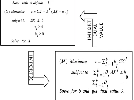
The following is a pictorial representation of the entire procedure discusses earlier. To carry on our calculation, at the very first time we have to randomly pick up an initial value of the dual variable and then solve the sub problem(s) from which we will import our current solution of the sub problem to create the master problem. After the creation of master problem, we have to solve the master problem and test the optimality condition. If the optimality condition does not hold, then we will take the current dual value from the master problem and import this to update our sub problem(s) and continue the same process unless we meet the optimality condition. We then have the following flow-chart.

Fig. 1. Flowchart of the algorithm. Showing the entire procedure

VI. NUMERICAL EXAMPLE

In this section, we present numerical examples to demonstrate our improved decomposition technique.

Following is a numerical example named Steelco problem

[10], for which we have shown the entire steps to solve the LP problem. In each step of solving master and sub problems, we used Lindo [11] to have the solution.

Let the LP is given by

(1)

(2)

3 (3)

(4)

(5)

Solution:

Applying the Lagrangean relaxation by relaxing constraint (5), we have the general single sub-problem and the associated master problem as follows

Sub-problem for iteration

3

Master problem for k-th iteration

∑

∑

∑

Now we are about to start the iterating process.

Iteration-1 (For k=1)

Starting value for (which is taken randomly)

Sub-problem

3

Solving by Lindo [10]gives and sub-problem value

Master problem

Solving by Lindo gives and master problem value , and the dual value for the next step is .

Since , thus the current solution is not optimal. Hence we proceed to the next iteration.

Iteration-2 (For k=2)

Sub-problem

3

Solving by Lindo gives and sub-problem value

Master problem

Solving by Lindo gives

and master problem value , and the dual value for the next step is .

Since , thus the current solution is not optimal. Hence we proceed to the next iteration.

Iteration-3 (For k = 3)

Sub-problem

Maximize

3

Solving by Lindo gives and sub-problem value

Master problem

Maximize

Solving by Lindo gives and master problem value , and the dual value for the next step is

Since , thus the current solution is not optimal. Hence we proceed to the next iteration.

Iteration-4 (For k=4)

Sub-problem

3

Solving by Lindo gives and sub-problem value

Master problem

Solving by Lindo gives and master problem value . Since , thus the current solution is optimal with the solution

∑

which gives with

VII. PROGRAMMING CODES IN AMPL In this section, we develop the computer code by the mathematical programming language AMPL to implement our improved decomposition technique.

Every AMPL [6] program is composed of three portions as model file, run file and data file. Model file contains the necessary parameter and variables declaration and the basic formulation. Data file and run files contain the inputs and formatting output commands respectively. For the above given example the corresponding model file, data file and run files are given below.

VII (A). MODEL FILE IN AMPL

# ---

# DANTZIG-WOLFE DECOMPOSITION

#

(steelcomod.txt)

# ---

param cr; #no. of complicating rows

param or; # no. of other rows

param nt; # no of thetas

param nsub; # no of subproblems

param nv; #no. of variables

param n_start {1..nsub}; #no. of variables

param n_end {1..nsub}; #no. of variables

param K >= 1 default 1;

#param complicatingConstraints {1..cr}; #param otherconstraints {1..or}; #param thetas {1..nt};

#param variables {1..nv}; param a{1..cr, 1..nv}; param b{1..cr}; param c{1..nv}; param d {1..or, 1..nv}; param f {1..or};

param lambda {1..cr} >= 0 default 100; param xl {1..K, 1..nv} >= 0 default 0; var Theta {1..nt, 1..K} >= 0;

var x {1..nv} >= 0;

### MASTER PROBLEM ###

maximize Master_ov : sum {s in 1..nsub, l in 1..K} Theta[s,l]*sum {i in n_start[s]..n_end[s]} c[i]*xl[l,i];

subject to Master_row {j in 1..cr}: sum{ s in 1..nsub,l in 1..K}

Theta[s,l]*sum {i in n_start[s]..n_end[s]} a[j,i]*xl[l,i] <= b[j];

subject to Convexity {j in 1..nt} : sum {l in 1..K} Theta[j,l] = 1;

### SUB PROBLEM ###

maximize Subproblem_ov {s in 1..nsub}: sum {i in n_start[s]..n_end[s]}c[i]* x[i]-sum {l in 1..cr}lambda[l]* (sum {i in n_start[s]..n_end[s]} a[l,i]*x[i] - b[l]);

subject to Subconstraints {s in 1..nsub, j in n_start[s]..n_end[s]}:

VII (B). DATA FILE IN AMPL

#

(steelcodat.txt)

param n_start := 1 1; param n_end := 1 4; param c :=

1 90 2 80

3 70

4 60 ;

param a : 1 2 3 4 :=

1 8 6 7 5 ;

param d: 1 2 3 4 := 1 3 1 0 0 2 2 1 0 0 3 0 0 3 2 4 0 0 1 1 ;

param b := 1 80 ;

param f := 1 12 2 10 3 15

4 4 ;

VII (C). RUN FILE IN AMPL

# ---

# DANTZIG-WOLFE DECOMPOSITION FOR # Steelco's problem with one subproblem # (steelcorun.txt)

# ---

reset;

model D:/steelcomod.txt; data D:/steelcodat.txt;

printf "\n\nStartTime %s.\n", ctime(); param iteration default 0;

param master_ov default Infinity; param subprob_ov default - Infinity;

problem Step1 {s in 1..nsub}: Subproblem_ov, x, Subconstraints;

problem Step2 : Master_ov, Theta, Master_row, Convexity;

printf "Default lambda = 100\n";

repeat while subprob_ov <> master_ov

{ let iteration := iteration + 1; let K:= iteration;

display iteration;

printf "Solve Subproblem.\n"; for {s in 1..nsub,

j in n_start[s]..n_end[s]} {

solve Step1[s];

let subprob_ov := Subproblem_ov[s]; for {i in n_start[s]..n_end[s]}

let xl[K,i]:=x[i]; }

printf "Solve master.\n"; solve Step2;

let master_ov := Master_ov; display iteration,subprob_ov,Theta, master_ov,lambda >

iterationsolution-steelco.txt; for {j in 1..cr} let lambda[j]

:= Master_row[j].dual; if subprob_ov - master_ov

<= 0.0001 then break;

display iteration; display subprob_ov; display master_ov; display lambda;

display Theta;

};

display subprob_ov; display master_ov; display xl;

display xl > iterationsolution-steelco.txt; display iteration;

display Theta;

for { i in 1..nv} printf"x[%i]=%g\n",i, sum {k in 1..K} Theta[1,k]*xl[k,i]; for { i in 1..nv} printf"x[%i]=%g\n",i,

sum {k in 1..K} Theta[1,k]*xl[k,i] > iterationsolution-steelco.txt; printf "CompletionTime %s.\n", ctime();

VII(D). COMMAND FOR GETTING OUTPUT

To get output, simply we have to write the following command:

VII (E). SUPPRESSED OUTPUT

In this section, we have shown the gist output of our concern which can be found as a text file inside the AMPL software folder.

iteration = 1 subprob_ov = 8000 Theta :=

1 1 1; master_ov = 0 lambda [*] := 1 100;

iteration = 2 subprob_ov = 1080 Theta :=

1 1 0.0909091 1 2 0.909091; master_ov = 981.818 lambda [*] := 1 0;

iteration = 3

subprob_ov = 1045.45 Theta :=

1 1 0 1 2 0.714286 1 3 0.285714; master_ov = 1000 lambda [*] := 1 12.2727;

iteration = 4 subprob_ov = 1040 Theta :=

1 1 0 1 2 0

1 3 -6.1089e-16

1 4 1;

master_ov = 1040 lambda [*] := 1 10;

x[1]=0 x[2]=10 x[3]=0

x[4]=4

VII (F). CONVERGENCE OF MASTER AND SUB PROBLEM

VALUES

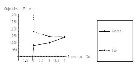
To obtain the graphical representation of the convergence of

master and sub problem values, we have used few commands

in MATHEMATICA [3] which gives us the following figure

to compare:

Fig. 2. Convergence of Sub-problem and Master-problem Value of Numerical Example 1.

VII. (G) RESULT COMPARISON

The values we calculated manually earlier and the values we have now from our programming output may be

tabulated as in Table I.

1.5 2 2.5 3 3.5 4 Iteration No . 950

1000 1050 1100 1150 1200 Objective Value

Table I Comparison of solutions

Iteration number Manual Output Program Output

1

2

3

4

Form the above table we can say that our computer program gives approximately the same results as we have for

manual technique. Moreover, the difference of getting the different results in just a few cases are caused by the

tolerance and internal difference of carrying operations between two Software Lindo and AMPL.

VIII (A). NUMERICAL EXAMPLE-2

2

VIII(B).DATA FILE FOR NUMERICAL EXAMPLE-2

param cr := 1;

param or := 4;

param nt := 1;

param nsub := 1;

param nv := 3;

param n_start := 1 1;

param n_end := 1 3;

param c :=1 10

3 4 ;

param a : 1 2 3 :=

1 10 4 5 ;

param d: 1 2 3 :=

1 1 1 1

2 2 2 6

3 1 2 3 ;

param b := 1 600

;

param f :=

1 100

2 300

3 400 ;

VIII (C). SUPPRESSED OUTPUT

iteration = 1

subprob_ov = 60000

master_ov = 0

lambda [*] :=

1 100;

iteration = 2

subprob_ov = 1000

master_ov = 600

lambda [*] :=

1 0;

iteration = 3

subprob_ov = 800

master_ov = 733.333

lambda [*] :=

1 1;

iteration = 4

subprob_ov = 733.333

master_ov = 733.333

lambda [*] :=

1 0.666667;

x[1]=33.3333

x[2]=66.6667

x[3]=0

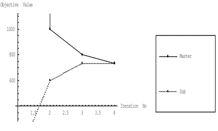
VIII (D).CONVERGENCE OF MASTER AND SUB

PROBLEM VALUES

To obtain the graphical representation of the convergence of master and sub problem values, we

have used few commands in MATHEMATICA [3] which gives us the following figure to compare:

Fig. 3. Convergence of Sub-problem and Master-problem Value of Numerical Example 2.

VIII (E). NUMERICAL EXAMPLE-3

VIII(F). DATAFILE FOR NUMERICAL EXAMPLE-3

param cr := 1;

param or := 3;

param nt := 1;

param nsub := 1;

param nv := 3;

param n_start := 1 1;

param n_end := 1 3;

param c :=

1 7

2 5

3 3 ;

param a :

1 2 3 :=

1

1 2 1 ;

param d: 1 2 3 :=

1 0 1 1

2 1 0 0

3 0 2 1 ;

param b :=

1

10;

param f := 1 5

2 3

3 8 ;

1.5 2 2.5 3 3.5 4 Iteration No

600 800 1000 Objective Value

VIII (G). SUPPRESSED OUTPUT

iteration = 1

subprob_ov = 1000

master_ov = 0

lambda [*] :=

1 100;

iteration = 2

subprob_ov = 42

master_ov = 38.1818

lambda [*] :=

1 0;

iteration = 3

subprob_ov = 47.7273

master_ov = 39.375

lambda [*] :=

1 3.81818;

iteration = 4

subprob_ov = 41.25

master_ov = 40

lambda [*] :=

1 2.625;

iteration = 5

subprob_ov = 40

master_ov = 40

lambda [*] :=

1 2;

x[1]=3

x[2]=2

x[3]=3

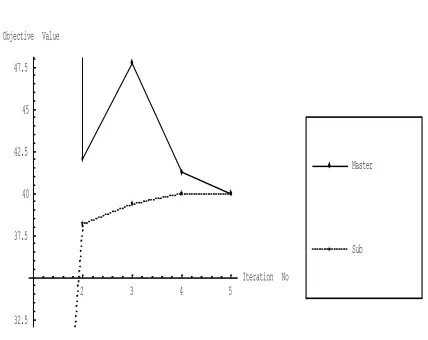
VIII (H). CONVERGENCE OF MASTER AND SUB

PROBLEM VALUES

To obtain the graphical representation of the convergence of master and sub problem values, we have used few commands in MATHEMATICA [3] which gives us the following figure to compare:

Fig. 4. Convergence of Sub-problem and Master-problem Value

IX. SOME REMARKS

Remark 1: The dual values taken in each case was a random choice. If we took the value of the dual variable as exactly we have in the iteration which gives optimal value, we would meet the optimal condition after a single iteration.

Remark 2: From the comparison in section VII (G), we faced some values disagree with results that we have using the manual process. This happens for the tolerance we set in our computer language in AMPL and for the round off procedure for taking the values of the solutions.

X. FURTHER WORKS

We are recently working on the following two works:

1. The procedure discussed in this paper is concerned with finding the optimal values of an LP. Currently we are working on the extension of the same procedure to find the optimal solution of an Integer Programming (IP).

2. The method discussed in this paper may be extended to find the optimal solution by decomposing the problem into any no of sub-problems.

XI. RESULT DISCUSSION

For solving the Steelco problem, as described in Winston [10], we experienced complex calculations of finding the extreme points, computation of

and the shadow prices which are clumsy and time consuming. But by our decomposition technique is

2 3 4 5

Iteration No

32.5 37.5 40 42.5 45 47.5 Objective Value

relatively an easier approach to carry on. It has the simple algorithm and computational strategy to find the optimal solution. Moreover, the computer codes in AMPL are available now which can help us to get the solution in a more compact form. Thus, our method has the notable advantages over the previous method.

XII. CONCLUSION

In this paper, we presented the modified decomposition algorithm for solving LPs which is also demonstrated with numerical examples. A computer technique for solving LP is also developed with proper instructions. After a comparative study between the methods taken into consideration in this paper, we conclude that our technique is more efficient for solving LP problems than the others.

REFERENCES

[1] Dantzig, G.B. and P. Wolfe (1961), “The Decomposition Algorithm for Linear Programming”, Econometrica, Vol. 29,

No.4.

[2] Dantzig, G.B. (1963), “Linear Programming and Extensions”, Princeton University Press, Princeton, U.S.A.

[3] Don, E. (2000), “Theory and Problems of Mathematica”,

Schaum’s Outline Series, Mc. GRAW-HILL.

[4] Fisher, M.L. (1979), “The Lagrangean Relaxation Method for Solving Integer Programming Problem”, Management Science, Vol. 27, No.1.

[5] Fisher, M.L. (1979), “The Lagrangean Relaxation Method for Solving Integer Programming Problem”, Management

Science, Vol. 27, No.1.

[6] Fourer, R., D.M. Gay and B.W. Kernighan (2003), “A Modeling Language for Mathematical Programming”, Second edition, Thomson Publication.

[7] Geofrion, A.M (1974), “Lagrange Relaxation for Integer Program”, Mathematical Programming Study, Vol. 2, pp. 82-114.

[8] Sweeny, D.J. and R.A. Murphy (1979), “A Method of Decomposition for Integer Programs”, Operations Research,

Vol. 27, No.6, pp. 1128-1141.

[9] Ravindran, Philips & Solberg (2000), “Operations Research”, John Wiley and Sons, Second Edition, New York, U.S.A.

[10] Winston, W.L. (1994), “Linear Programming: Applications and Algorithm”, Duxbury press, Belmont, California, U.S.A.